Bearing Fault Classification of Induction Motors Using Discrete Wavelet Transform and Ensemble Machine Learning Algorithms

Abstract

Bearing fault diagnosis at early stage is very significant to ensure seamless operation of induction motors in industrial environment. The identification and classification of faults helps to undertook maintenance operation in an efficient manner. This paper presents an ensemble machine learning-based fault classification scheme for induction motors (IMs) utilizing the motor current signal that uses the discrete wavelet transform (DWT) for feature extraction. Three wavelets (db4, sym4, and Haar) are used to decompose the current signal, and several features are extracted from the decomposed coefficients. In the pre-processing stage, notch filtering is used to remove the line frequency component to improve classification performance. Finally, the two ensemble machine learning (ML) classifiers random forest (RF) and extreme gradient boosting (XGBoost) are trained and tested using the extracted feature set to classify the bearing fault condition. Both classifier models demonstrate very promising results in terms of accuracy and other accepted performance indicators. Our proposed method achieves an accuracy slightly greater than 99%, which is better than other models examined for the same dataset.

1. Introduction

Among rotating machinery, induction motors (IM) are broadly used in manufacturing industries such as transportation, petrochemicals, and power systems due to low cost, high reliability, robust design, and higher efficiency under full load. Generally, IMs need to remain operative for a long duration and commonly under harsh operating environments accompanied with regular wear, which cause mechanical and electrical stresses. These can lead to unexpected failure in gears and bearings, which are the significant machine components of IM. Such failures could cause financial losses or human causalities. Therefore, machine health monitoring and fault analysis become an integral part of the maintenance system in an industrial environment. A robust condition monitoring system can decrease maintenance charges, improve productivity, and increase reliability and safety. In recent times, the machine learning (ML)-based fault analysis approaches are turned out as a powerful and prevalent approaches in the area of continuous health monitoring of rotating machineries, as they have the ability to extract valuable information from the considerable amount of historical data [1,2,3].

Rotor faults, stator faults, rolling element bearing (REB) faults, and other faults commonly occur in IMs, among them bearing faults are most frequent. Statistics shows that 40% of total breakdown situation in large size machines occurred due to bearing fault and the number is as high as 90% in case of small machines [4]. The main elements of a bearing are the inner, and outer ring, rolling element, and cage. Faults in bearings may occur during manufacturing or after some period of operation. If a defect occurs on a contact surface of the bearing elements, an impact is generated when the bearing hits the defect, which results a strident transient response followed by damped oscillation. Generally, the periodic transient behavior contains important information regarding bearing health [5]. Therefore, detecting the transient response and accurate analysis of the signal can successfully forecast bearing faults in the early state. This is crucial for preventing unpredicted downtime of rotating machines and for confirming safety without affecting the efficiency of the industrial process. Hence, real-time monitoring and diagnosis approaches for REB have gained considerable attention from researchers in recent years. Reactive, preventive, and predictive maintenance are the three primary approaches for fault diagnosis. In reactive maintenance, the fault occurs, and then initiates corrective measures, which results in failure of the machine, high cost of components, reduced safety, and unanticipated downtime. The preventive maintenance process aims at a time bound procedure and designs a corrective action periodically without knowing the real time condition of the REB, which requires many resources and a lower efficiency. Lastly, predictive maintenance is designed based on real-time monitoring and performance of necessary actions when the REB shows a certain behavior that indicates failure or diminished performance [6]. From another point of view, fault diagnosis can be divided into model-based and knowledge-based methods. The system faults are analyzed by an equivalent mathematical model of the system; however, this can be complicated by system non-linearity. On the other hand, knowledge-based methods are developed depending on measurements, experience, data analysis, and physical assessment of the target structure [7].

Developments in sensors, communication technology, availability of data, and an efficient data processing algorithm have suggested data- or knowledge-based fault diagnosis condition monitoring system as a more acceptable choice. The data-driven fault diagnosis system, data acquisition, data preparation, construction of feature matrix, and fault classification are the four most popular phases.

Condition data for IMs can be collected in different forms as acoustic emission [8], vibration, temperature readings, current sources, and thermal images, which are extensively investigated for bearing fault investigation [9]. Recently, vibration signal analysis for fault analysis has gained much attention for monitoring health of the machine due to the capacity to transfer intrinsic information of mechanical systems [10,11]. External vibration sensors (e.g., accelerometers) are required to be mounted around the bearing, which are very costly, and the installation process requires full time access to the IM. Because of these drawbacks, the bearing based on vibration-signal is not easily accessible in remote locations or for a less complex system. On the other hand, using current signal for condition monitoring offers some advantages over the vibration signal as it does not require external sensors for data collection. Moreover, if there are no frequency inverters or current transformers, the stator current from a single input source can be measured with the help of current transducers [12]. Hence, due to the cost-effective and noninvasive nature, motor current signal analysis (MCSA) is considered one of the most proficient condition monitoring techniques. Also, multiple signature analysis combining motor current and vibration signal analyses has been performed to ensure higher reliability [13].

From the raw data fault, classification or identification is not possible. With various signal processing techniques, the sensor data are analyzed by extracting fault information. Some widely used approaches for signal analysis are time-domain analysis [14], frequency-domain analysis [15], enhanced frequency analysis [16], and time-frequency analysis techniques [17]. The techniques based on signal processing do not need any equivalent circuit model, and the performance of the system depends on the working condition of the machine. Therefore, the computational cost may increase if complexity of the advanced signal processing tool is increased. The root mean square, short impulse method, and high-order statistics are some of the frequently used time-domain techniques. In frequency-domain analysis, Fast Fourier transform (FFT), envelope analysis, and high-order spectral analysis [18] are generally used. FFT is the most widely used method due to less computational complication in comparison with the other methods. For any signal with non-stationary nature, which is common, frequency domain analysis is not widely applicable because it is not able to reveal the intrinsic information. Generally, the running machine contains many non-stationary components because of environmental change and faults from the machine itself. Therefore, it is significant to evaluate the signals with non-stationary type, with the help of various time-frequency analyses, such as short-time Fourier transform (STFT), the Wigner-Ville distribution (WVD), and wavelet transform. Application of this technique revealed both the time and frequency domain information necessary for investigation.

In machine learning-based fault analysis, signal processing is generally used for signal conditioning and feature extraction and include cyclic spectral analysis [19], statistical analysis, [20] wavelet analysis [21,22,23], Hillbert-Hung transform [24], and correlation [25]. Therefore, because of the exclusive characteristics of wavelet analysis, it is used widely for analyzing non-stationary signals. It is used for fault diagnosis in gears and bearings [26,27], locating fault and crack size determination in different structures and components [28,29]. In detection and extraction of features for fault classification, many researchers reported successful implementation of wavelet transform [30,31,32]. Various types of faults in the power system [33] are successfully differentiated from three-phased voltage signal decomposition up to only 4th level using DWT. Although many variations of wavelet functions exist, it is crucial to choose a suitable wavelet to find out the best match and extract the most suitable features. After the initial signals are transformed into a compact relevant representation, they are act as input of a classifier to train and improve the decision function. Among the various processes of classification, Support Vector Machine (SVM) and Artificial Neural Network (ANN) are mostly implemented for machine fault detection and identification [34,35,36,37].

Now a days, extreme learning machine (ELM), a neural network having single hidden-layer-feed-forward has been implemented [38] for fault detection and classification and has a very fast learning rate and higher accuracy for prediction in comparison with SVM and ANN. Recently, deep learning (DL) approaches have been considered for fault diagnosis. The DL technique consists of multiple levels of non-linear operation and can automatically learn up to high-level features to allow decision-making more intelligently. DL methods, such as the Deep Belief Networks (DBN), Stacked Auto Encoders (SAE), and Convolutional Neural Network (CNN), have been investigated recently in fault diagnosis [39,40,41,42]. Despite attaining an effective solution from ML techniques, these methods often become stacked in a local minimum, if the configuration parameters are not efficiently considered [43]. In recent times, researchers have started to apply a modernized approach known as ensemble learning to avoid the drawbacks of ML approaches such as feature selection, incremental learning, class-imbalance data, as well as learning concept drift from non-stationary distributions [44]. Ensemble learning is one example of the ML prototypes where multiple learners need to be trained for solving a single problem. Moreover, this method provides better generalization to adapt to any unknown case, better efficiency of avoidance from local minima, and greater search abilities than any ordinary ML approach. Random forests and extreme gradient boosting (XGBoost) are two well-known ensemble ML methods proposed by Breiman [45] in 2001 and Dr. Chen Tianqui [46] in 2014, respectively. The XGBoost algorithm possesses low computational complexity, high accuracy, and fast running speed for any input data set size due to utilization of the central processing unit (CPU) with multi-threaded parallel computing. These methods are effectively used in various fields, such as prediction of environmental condition, detection of medical symptoms, and diagnosis of machine faults [47,48,49].

In this study, we used three types of discrete wavelet transform (DWT) for signal decomposition. Later, statistical features were calculated from the high-level approximation coefficients and the detail coefficients to reduce the feature matrix dimension. After that, to estimate the performances, two ensemble learning algorithms, RF and XGBoost, were trained to classify. Finally, a comparison is made with some recent works on motor current signal, where Lessmeier et al. [50] applied particle swarm optimization based support vector machine (SVM-PSO) and in [51,52], the authors used deep learning based approaches for IM fault classification.

Therefore, the main contributions of this paper can be listed as follows:

• Evaluate the performances of various wavelets for motor current signal analysis.
• Observe the effect of denoising the current signal on classification accuracy.
• Evaluate the performance of two ensemble classifiers for bearing fault identification of an IM.

The remainder of this paper is organized as follows. Section 2 provides a description of the experiment set up and characteristics of the data. Section 3 describes the overall process of the method utilized in this paper. Section 4 explains the experimental results and performance of the proposed approach using the evaluation parameters from the dataset, and Section 5 concludes the paper.

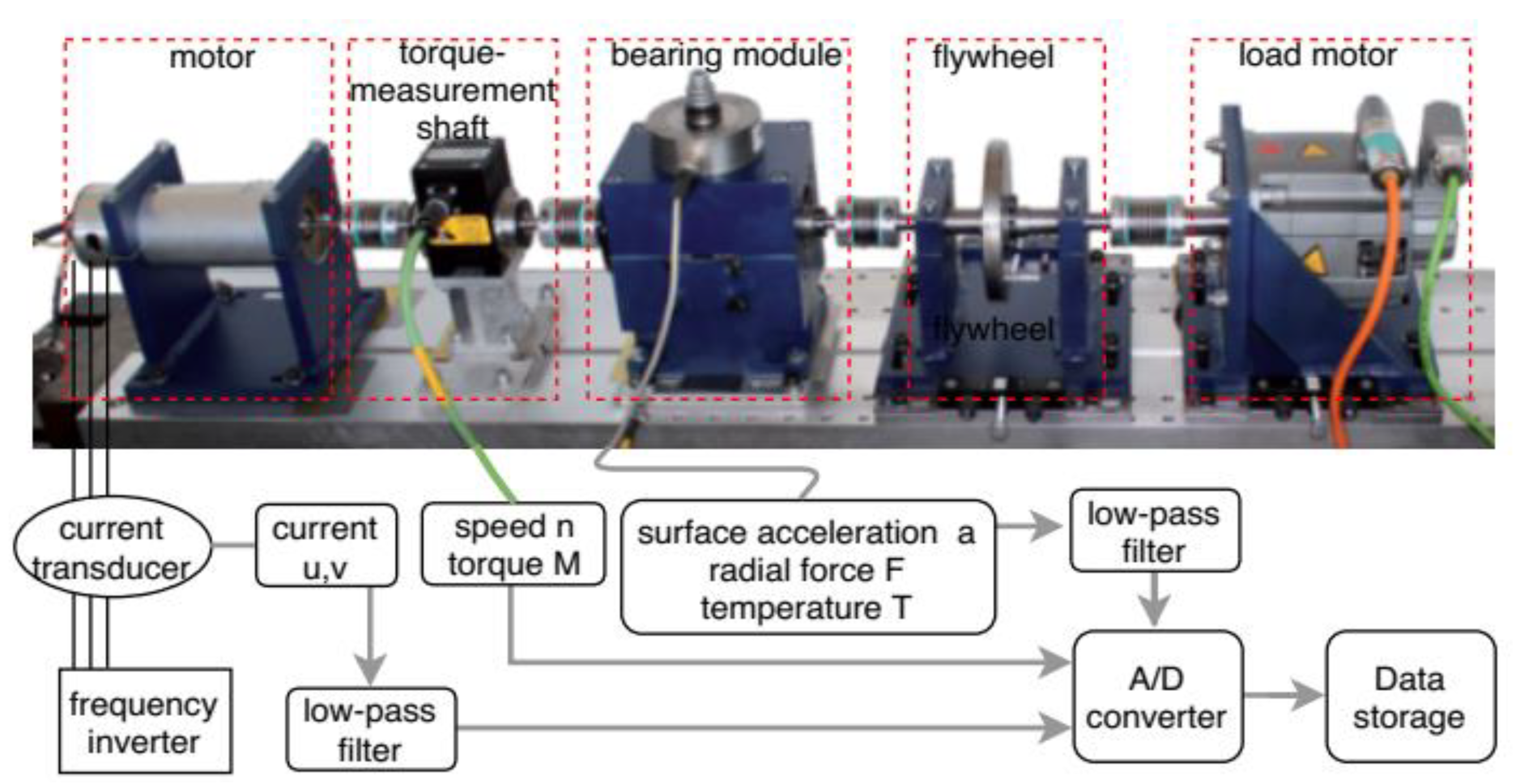
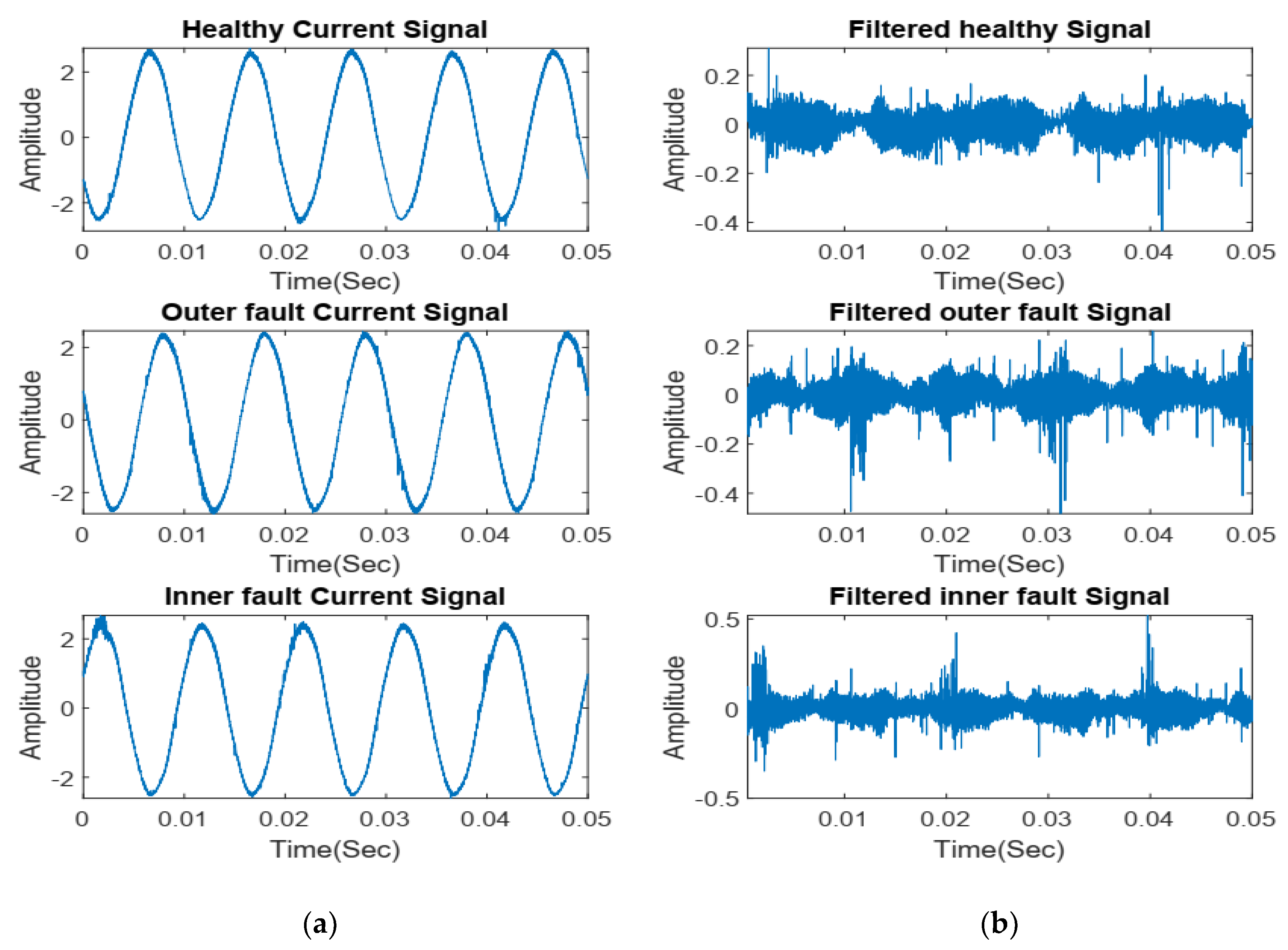
2. Experimental Test Rig and Data Description

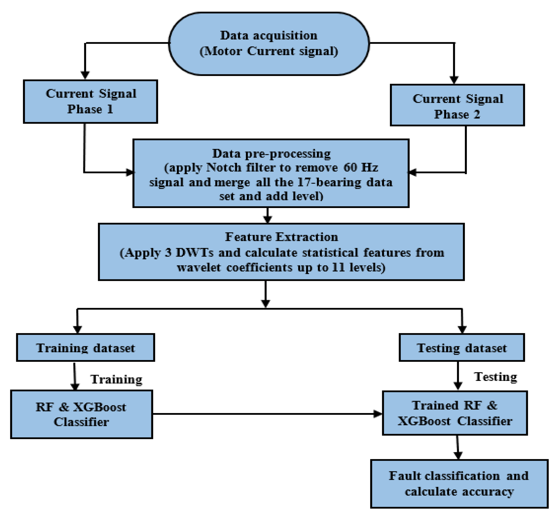
The data set used in this work for is collected from the bearing datacenter administrated by faculty of mechanical engineering, Paderborn University, Germany. The overall data were acquired from 32 experimental bearings and were classified into healthy, artificially damaged bearings, and real damaged bearings with an accelerated lifetime test. The testbed is shown in Figure 1 and consists of a permanent magnet synchronous motor, operated by a frequency inverter with a switching frequency of 16 kHz. Along with motor currents and vibration, other supportive measurements named as speed, torque, temperature, and radial load are also available [50].

The test rig was driven under several working conditions to diversify the dataset. The working conditions are listed in

Table 1. Operating Conditions.

No.	Rotational Speed	Radial Force	Load Torque
	(S)	(F)	(M)
	[rpm]	[N]	[Nm]
1	1500	1000	0.7
2	1500	1000	0.1
3	900	1000	0.7
4	1500	400	0.7

. The damage size, location, geometry, and occurrence in the test rig followed the ISO 15243(2010) standard.

In our study, among the 32 bearings, we considered the motor phase currents of two phases (CS1 and CS2) from 17 bearings which include healthy bearing and those with inner and outer race faults as mentioned briefly in

Table 2. Bearings considered in this work and their condition.

Type of Bearing		Bearing Code	Damage (Main Mode & Symptoms)	Label
Healthy Bearing Data		K001	-	0
		K002	-
		K003	-
		K004	-
		K005	-
		K006	-
Naturally Damaged Bearing Data	Outer Ring	KA04	Fatigue: pitting	1
		KA15	Plastic deformity: Indentations
		KA16	Fatigue: pitting
		KA22	Fatigue: pitting
		KA30	Plastic deformity: Indentations
	Inner Ring	KI04	Fatigue: pitting	2
		KI14	Fatigue: pitting
		KI16	Fatigue: pitting
		KI17	Fatigue: pitting
		KI18	Fatigue: pitting
		KI21	Fatigue: pitting

. The current signal is recorded with a current transducer (LEM CKSR 15-NP). For each setting, there are 20 files containing 4 s of data, saved in mat file format. In our analysis, we considered the current signal of 1 s rather than the whole 4-s duration for both phases. The sampling frequency was set at 64 kHz; therefore, the initial dataset is a matrix of size 2720 × 64,000.

Time domain representation of current signals recorded from three bearings (healthy bearing, bearing with inner ring fault, and bearing with outer ring) are provided in Figure 2. The time domain signal depicts very subtle changes among the three signals. The frequency spectrum is presented in Figure 3, which reveals that each signal contains a 60 Hz component. This is the line/characteristic frequency. We evaluated the classifier performance with and without this 60 Hz component, which will be discussed in a later section.

3. Methodology

The main objective of this work is to explore the appropriateness of ensemble learning to motor bearing fault analysis using the current signal. To create a relevant feature matrix to train the classifiers, the raw current signals are passed through a notch filter and decomposed using three wavelets.

The purpose of using three wavelets is to observe which wavelet decomposition provides a better performance for feature extraction. The feature matrix is constructed by computing 11 features from the wavelet coefficients. Finally, the classifier model is validated by a cross-validation method. Several hyperparameters for each classifier are also determined to ensure optimum performance. A generalized workflow is presented in Figure 4.

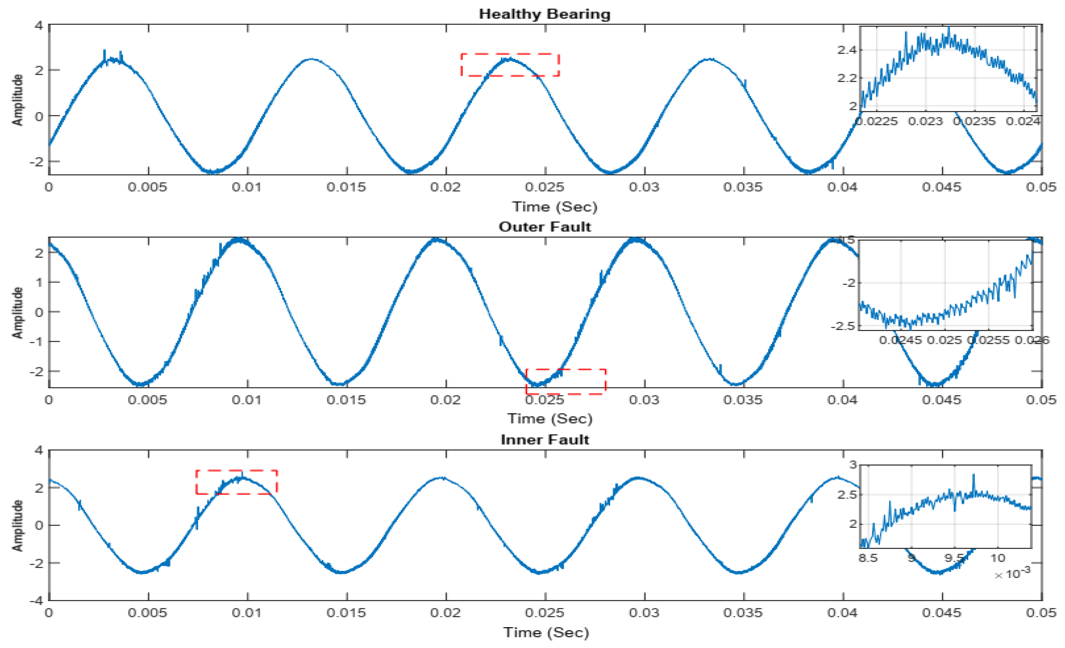
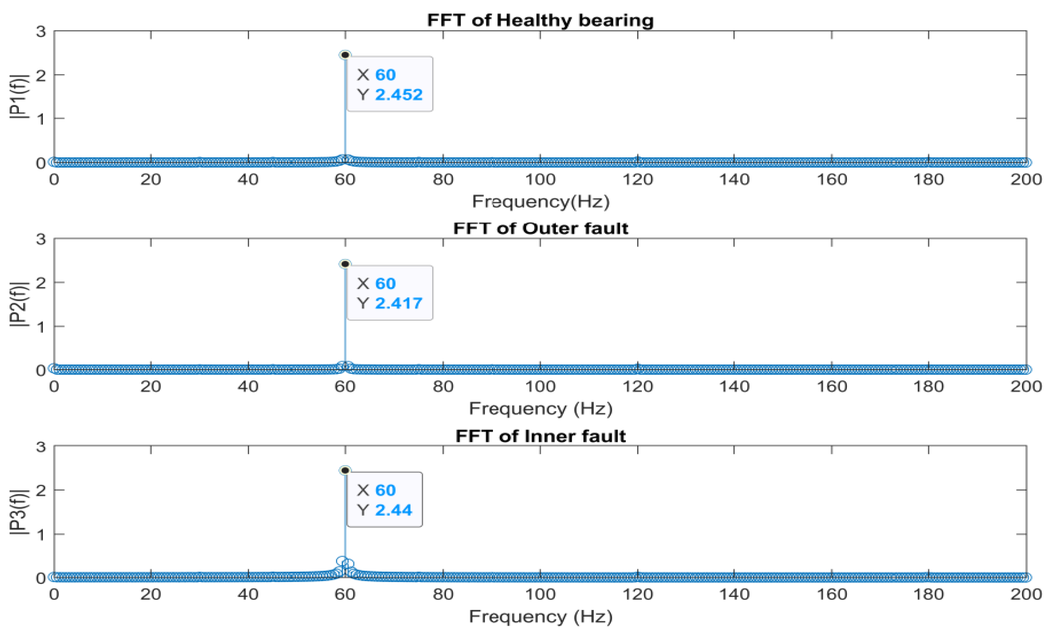
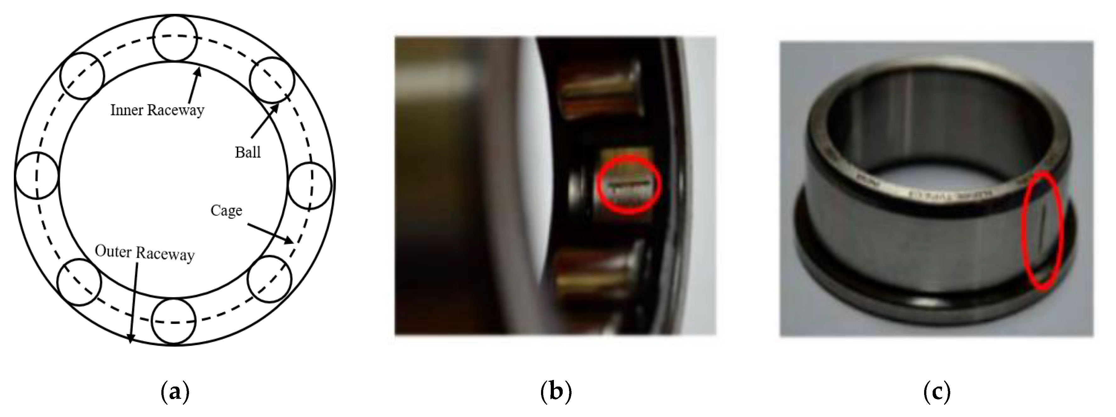
3.1. Bearing Fault Signatures

The rolling element bearing (REB) is an important component in rotating machines and generally carries heavy loads with expectations to operate at high reliability and efficiency. Usually, the inner ring and outer ring of the bearing are mounted on a rotating shaft and stationary housing, respectively. The balls, tapered rollers, cylindrical rollers, and barrel rollers are the rolling elements, enclosed in a cage with equal spacing. To allow the rolling element to contact the ring at a single point, the radii are slightly smaller than the track of rotation and help to distribute the load to a very small surface. General representation of rolling element bearing, and two different types of fault analyzed in this study are represented in Figure 5.

Therefore, the cage isolates the rolling elements to avoid bad lubrication surroundings through the operation. A large variety of REBs exists, including the deep groove ball bearings, and are mostly used in home appliances, industrial equipment, and automotive applications. Various types of damage such as pitting, spalling, waviness, and misaligned races generally occur due to abrasive wearing, improper installation, material fatigue, manufacturing error, and so on.

Generally, each bearing element obtains a representative frequency. When damage occurs on a bearing element, the interaction of defects produces pulses of very small duration, which result in a rise in vibration energy at that particular frequency. The damage frequency can be determined with the help of the geometry of the bearing and element rotational speed from Equations (1)–(4).

$$\mathrm{Outer}\mathrm{race}\mathrm{defect}:f_{outer}=\frac{N_{ball}}{2}\times f_m\times \left(1-\frac{D_{ball}}{D_{cage}}\times \cos (\beta )\right)$$

(1)

$$\mathrm{Inner}\mathrm{race}\mathrm{defect}:f_{inner}=\frac{N_{ball}}{2}\times f_m\times \left(1+\frac{D_{ball}}{D_{cage}}\times \cos (\beta )\right)$$

(2)

$$\mathrm{Ball}\mathrm{defect}:f_{ball}=f_m\times \frac{D_{cage}}{D_{ball}}\times \left(1-\frac{D_{ball}^2}{D_{cage}^2}\times \cos (\beta )\right)$$

(3)

$$\mathrm{Cage}\mathrm{defect}:f_{cage}=\frac{1}{2}\times f_m\times \left(1-\frac{D_{ball}}{D_{cage}}\times \cos (\beta )\right)$$

(4)

where β, N_ball, D_ball, D_cage and f_m represent the contact angle of the balls, the number of balls or cylindrical rollers, the diameter of the ball, the cage diameter (also known as the roller or ball pitch diameter), and the rotational frequency, respectively. The detailed ball bearing geometry was described in [53].

Characteristic fault frequencies induce the current signals and oscillations because bearing damage changes the radial motion between the rotor and stator. Therefore, fluctuations of rotating eccentricity and load torque also occur as bearing damage produces radial displacement of the rotor relative to the stator and results in amplitude, phase, and frequency modulation of the motor-current signals. The bearing fault motor current equation is described in [54] as:

$$i(t)={\displaystyle \sum _{k=1}^{\infty }{i}_k}·\cos ({\omega }_{c_k}t+\mathsf{\phi })$$

(5)

where φ and ${\omega }_{c_k}$ represent the phase angle and angular velocity, respectively, and

$${\omega }_{c_k}=\frac{2\pi f_{bearing}}{p}$$

$$\mathrm{where},f_{bearing}=\left|f_s\pm m{f}_v\right|$$

(6)

Here, f_bearing, p, and f_s denote harmonic frequency of the fault current, the pole pair number of the corresponding machine, and fundamental frequency, respectively. The fundamental frequency is referred to as the electrical supply frequency. This is the frequency of three phase power supply connected to the stator of the induction motor. Hence, m = 1, 2, 3, … are the harmonic indexes; and f_v can be f_inner, inner race frequency, or f_outer, outer race damage frequency. However, the noise frequency and harmonics produced by the bearing fault become very close or tend to overlap each other, complicating bearing fault detection [55]. In our study, we analyzed three types of bearing conditions: healthy, inner race fault, and outer race fault.

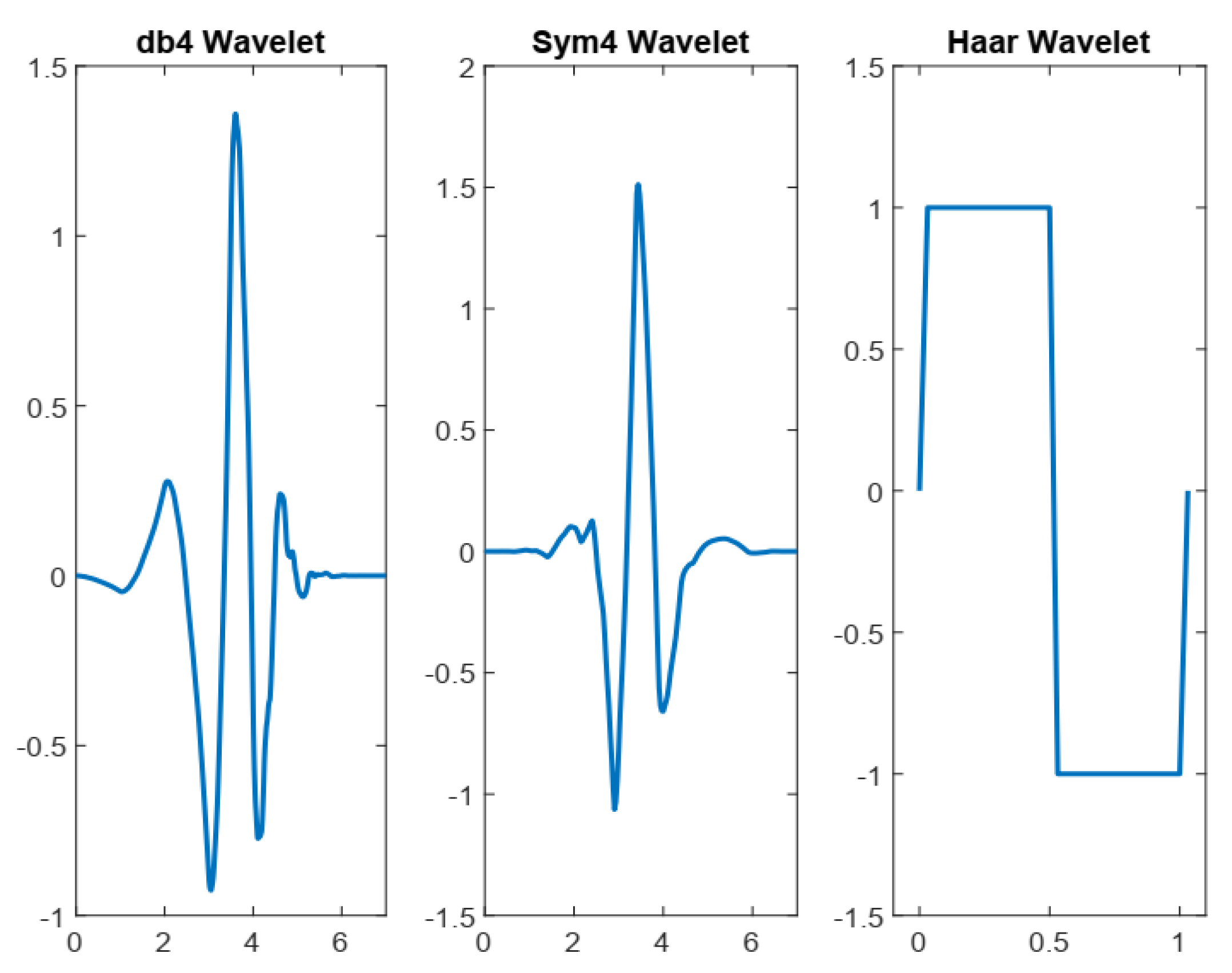
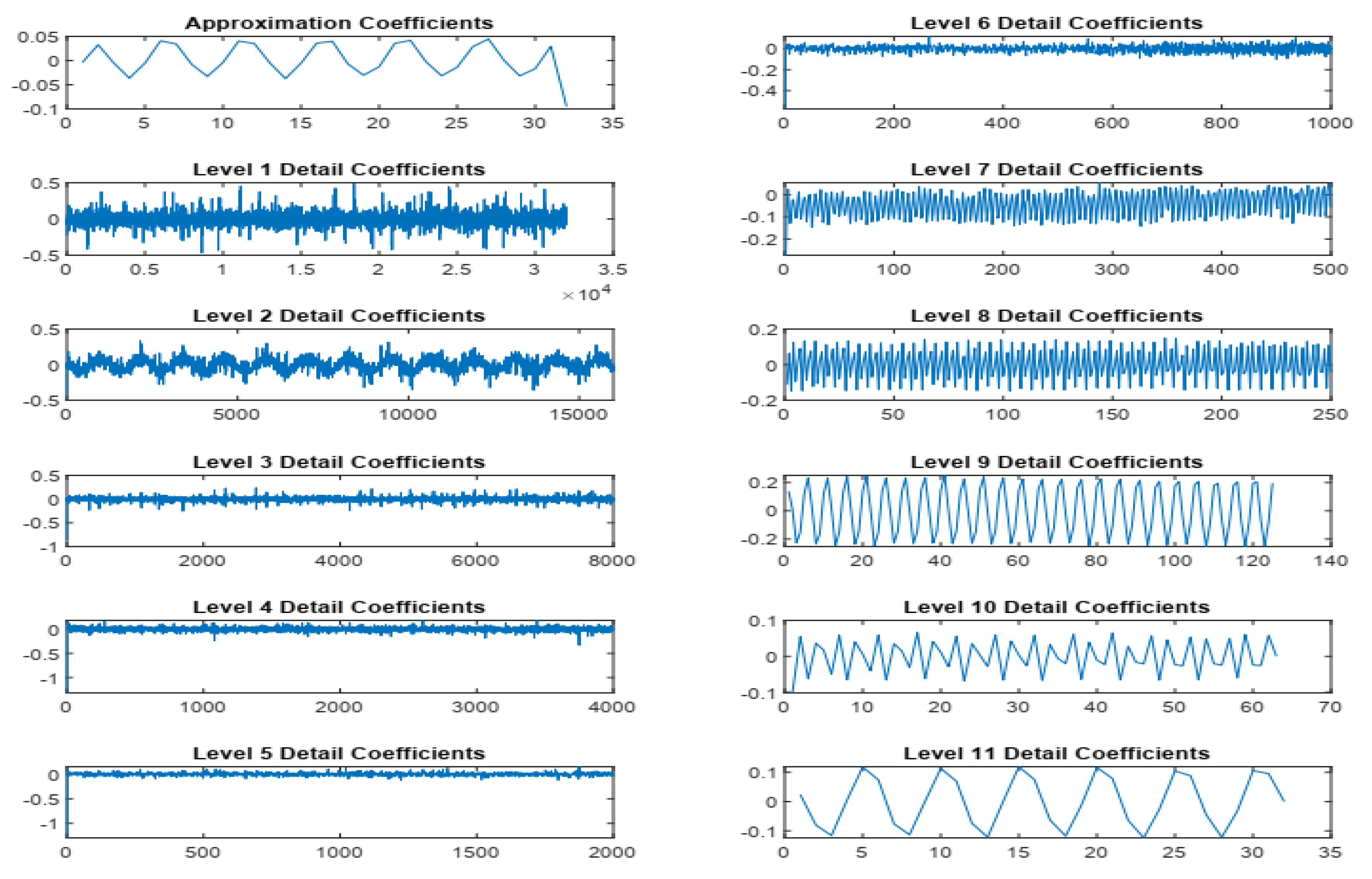
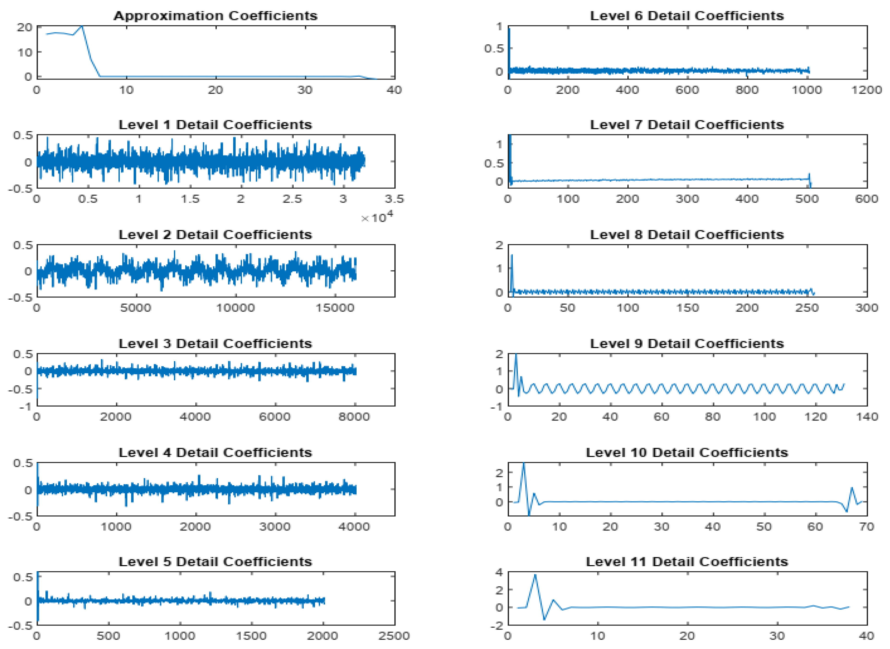
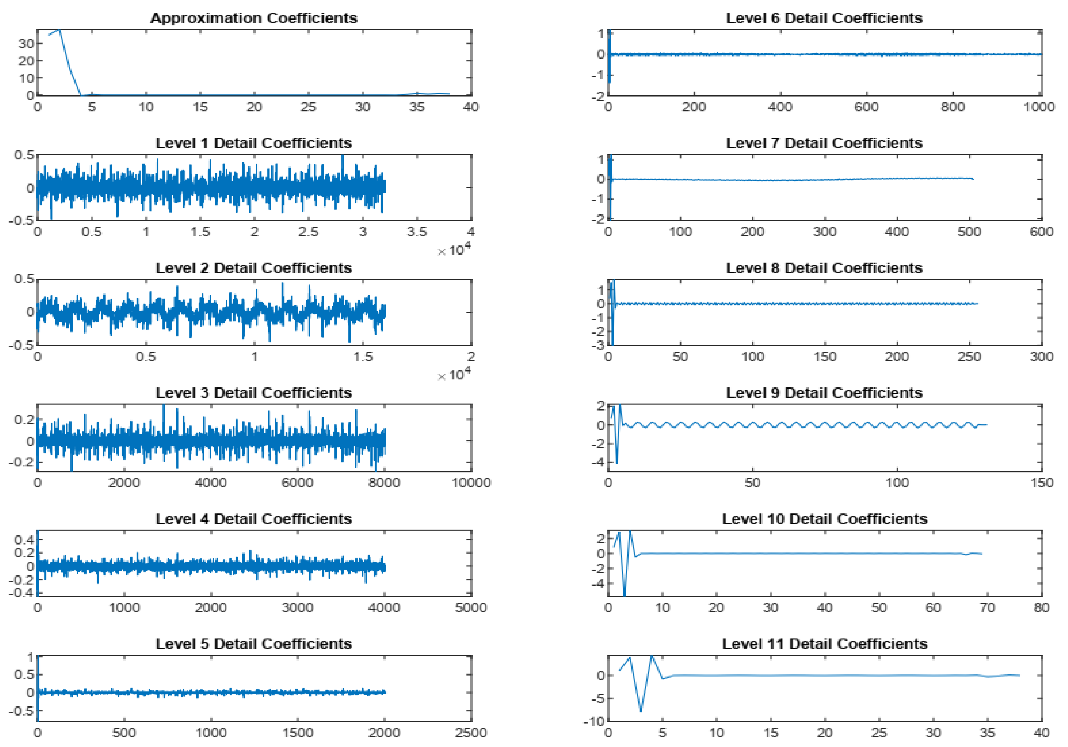
3.2. Wavelet Transform

Though frequency information in Fourier transform is extracted for a whole duration of the signal, it is normally determined by calculating the average over the complete length of the signal, which is a major drawback of Fourier transform [56]. To overcome this problem, many time-frequency domain approaches have been used, such as Gabor transform, short-time Fourier transform (STFT), Wigner–Ville transform, and wavelet transform. Among them, wavelet transform is based on Fourier transform and STFT to allow transformation of the time domain signal into time-frequency domain. In wavelet transform, small signals are mathematically integrated into one complete signal, and the small signals are known as wavelets. The wavelet is a short duration oscillation starting and ending at zero. There are several orthogonal basis functions which are known as the mother wavelets. Number of other wavelets are created from wavelet by scaling (stretching or shrinking) with the mother wavelet itself. The shifting of scaled wavelets along the time axis provides information about localization of different frequency contents of the corresponding signal. There are two variants of wavelets namely continuous wavelet transform (CWT) and discrete wavelet transform (DWT).

The CWT is defined in [57] as

$$CW{T}_{(a,b)}(t)=\frac{1}{\sqrt{a}}{\displaystyle \underset{-\infty }{\overset{+\infty }{\int }}x(t){\psi }^{*}(\frac{t-\tau }{a}})dt$$

(7)

where a, $\tau$, and $\psi$ represent the scale parameters, translation parameter, and mother wavelet, respectively. $\psi$* is the complex conjugate of $\psi$.

The DWT is derived from discretization of CWT (a,b) as

$$DW{T}_{(j,k)}(t)=\frac{1}{\sqrt{2^j}}{\displaystyle \underset{-\infty }{\overset{+\infty }{\int }}x(t){\psi }^{*}(\frac{t-2^{j}k}{2^j}})dt\mathrm{where},a=2^j\mathrm{and}\tau =2^{j}k$$

(8)

Generally, a multiresolution analysis decomposes the signal into a smoother version of the original signal (approximations) and a set of detailed information at various scales. Here, j and k can be any positive integer values such as 1,2, 3, … The high frequency and low frequency components are known as detail coefficients (cD) and approximate coefficients (cA), respectively. This process is performed using a series of high and low pass filters and can be expressed as

$$x(t)=A_j+{\displaystyle \sum _{j\le J}{D}_j}$$

(9)

where A_j and D_j represent the low frequency bands (approximations) and high frequency bands (details) of the signal, respectively. At the transient state, the high frequency components will be evaluated to analyze the signal. In addition, the DWT exposes aspects of data such as discontinuities of higher derivatives, breakdown point, and self-similarity in a more efficient manner than any other signal processing technique.

A number of mother wavelets exists for both CWT and DWT all of them are not equally applicable for any signal. It is the nature of signal (e.g., image, time-series data) and field of application which influences which wavelet to be used. Researchers need to look for the wavelet function that best correlates with the function or signal being analyzed to extract the most effective information. As found in the literature, for time-series signals, Haar, db4, and sym4 wavelets are widely used [23,58], as is represented in Figure 6. Therefore, we explored the effectiveness of these three wavelets in decomposing motor current signal-based fault analysis.

Among them, the Daubechies (db) and Symlets (Sym) show asymmetric basic function, where the Haar wavelet possesses absolute symmetry in nature.

3.3. Feature Extraction

The dataset at its primary state is quite large, but it is useful in training a classifier model. However, the dimensionality of the input data should be as small as possible to obtain high classification accuracy with low computational resources. Often, based on application and amount of available data, feature extraction can be omitted, and the data are directly used to train the classifier. In the feature extraction technique, the data dimension is reduced from the initial data by transferring it into a smaller and more tractable set of data for future processing. In the raw data set, because of the different types of working conditions and machine inputs, the number of variables becomes very large and will demand higher computing resources for the next step. The main objective of feature extraction is to convert the raw data into a smaller subset of significant variables that efficiently represent the target classes. Thus, feature extraction is a crucial step for easier calculation and reservation of important information for ultimate decision making.

Before performing feature extraction from the current signals, the line component of the 60 Hz component is removed using a notch filter. Then data from 17 bearing conditions are merged. The raw signal and the filtered signal for three bearing conditions are shown in Figure 7. It is not easy to differentiate between faulty and healthy condition signals from the non-filtered signals by visual inspection, but the filtered version is more discernable.

The filtered signal is decomposed up to 11 levels with each of the Haar, db4, and sym4 wavelets. From the 11-level decomposition, we obtained the detailed coefficients from level 1 to 11 (cD1 to cD11) and one approximation coefficient (cA) for each wavelet. The decomposed signals are presented in Figure 8, Figure 9 and Figure 10.

Due to the high dimension of data containing an excessive amount of information, wavelet decomposition coefficients cannot be directly used as the input of classifiers. To reduce the data dimension and extract the most important characteristic information, feature extraction methods are applied to the wavelet coefficients at every decomposition level.

In this study, 11 statistical features are used for feature extraction from 11 approximation coefficients and the detail coefficient of each wavelet. The initial dataset has 2720 instances containing three different conditions of bearing (healthy, inner race fault, and outer race fault). Each instances is essentially a current signal having a duration of 1 s, sampled at 64 KHz. In the feature extraction stage, each instance is decomposed to 11 levels. Therefore, after decomposition for each instance there are 11 detail and 1 approximation coefficients (total 12 coefficients). Thus, for each coefficient, the features mentioned in

Table 3. The formulae used for feature extraction from the current signal (x represents the signal vector).

Techniques for Extracted Feature	Feature Number (k)	Equations of Detailed & Approximation Coefficients
1. Mean	k = 1, …, 12	$\mu =\frac{1}{N}{\displaystyle \sum _{i=1}^N{x}_i}$	(10)
2. Standard deviation	k = 13, …, 24	$\sigma =\sqrt{\frac{{\displaystyle \sum _{i=1}^N{(x_i-\mu )}^2}}{N-1}}$	(11)
3. Skewness	k = 25, …, 36	$x_{skewness}=\frac{1}{N}\frac{{\displaystyle \sum _{i=1}^N{(x_i-\mu )}^3}}{{\sigma }^3}$	(12)
4. Kurtosis	k = 37, …, 48	$x_{kurtosis}=\frac{1}{N}\frac{{\displaystyle \sum _{i=1}^N{(x_i-\mu )}^4}}{{\sigma }^4}$	(13)
5. RMS	k = 49, …, 60	$X_{rms}=\frac{\sqrt{{\displaystyle \sum _{i=1}^N{x}_i{}^2}}}{N}$	(14)
6. Form factor	k = 61, …, 72	$F_f=\frac{\mu }{X_{rms}}$	(15)
7. Crest factor	k = 73, …, 84	$C_f=\frac{X_{\max }}{X_{\min }}$	(16)
8. Energy	k = 85, …, 96	$E={\displaystyle \sum _{i=1}^N{x}_i{}^2}$	(17)
9. Shannon- entropy	k = 97, …, 108	$H_s=-{\displaystyle \sum _{i=1}^N{x}_i{}^2}\log (x_i{}^2)$	(18)
10. Log-energy entropy	k = 109, …, 120	$H_e=-{\displaystyle \sum _{i=1}^N\log (x_i{}^2)}$	(19)
11. Interquartile range	k = 121, …, 132	$IQR=x_i(\%75th)-x_i(\%25th)$	(20)

are calculated, which is 12 × 11 = 132 features. Finally, after adding the label at the last column, we have a feature matrix of 2720 × 133.

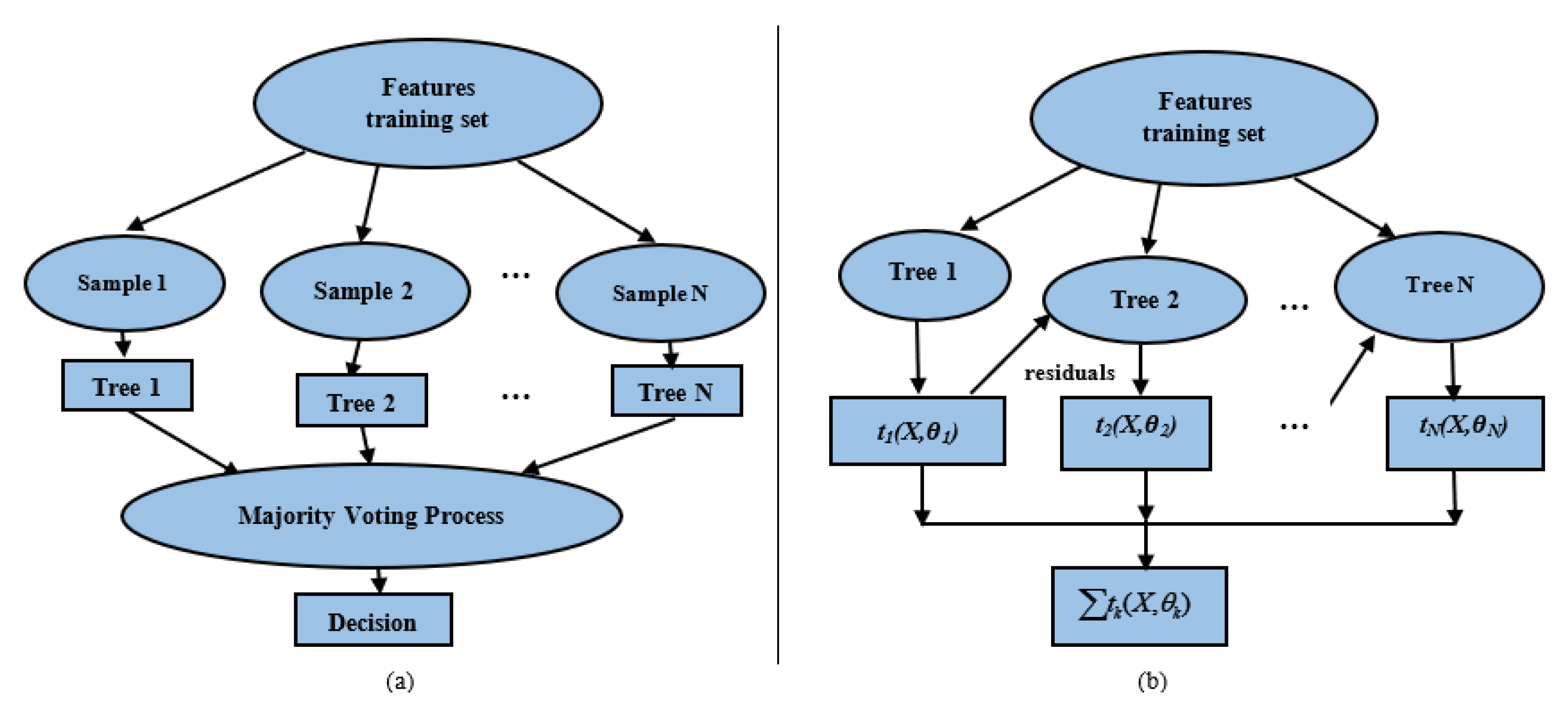
3.4. Ensemble Learning

In recent times, selection of an efficient ML algorithm has become crucial for good performance of any fault diagnostic model. Ensemble learning algorithms are one of the approaches that provide better performance than any single prediction algorithm [59]. In ensemble learning, multiple weak learners work together to produce a better model achieving higher accuracy. Some ensemble learning algorithms such as XGBoost may achieve higher accuracy than artificial neural networks and degree-day ordinary least square regression for energy model loss estimation [60]. In our study, two ensemble learning algorithms known as random forest and XGBoost were investigated for fault classification of IM.

3.4.1. Random Forest

The Random forest (RF) algorithm is a collection of decision tree, where each tree is individually trained on an arbitrarily selected independent training dataset. Here, the respective input dataset for each tree is sampled separately, and the distribution rate is the same for all trees. RF not only performs well in classification and regression, but also shows outstanding performance in variable selection. The trees are obtained from the combination of datasets with bootstrap subsampling and various subsets of features for splitting at every node. The nature of each tree is unique and possesses low bias when mature. Also, low correlation is obtained based on selection of random subsets of features for the individual trees. Finally, after ensemble of all the trees, the RF results in low bias and low variance for the model. Bootstrap aggregating from bagging is designed to increase the stability and accuracy for individual trees in RF [48]. For decision making, the class which receives majority vote from the trees is selected in classification problem. On the other hand, the average of the predicted values from all decision trees is considered in regression models. The RF can also overcome the overfitting problem, which is one of the main concerns in a decision tree algorithm. RF uses a bagging technique, where each time a random subset of feature is used to train a single decision tree and it aggregates the result of a number of decision trees to determine the final output. Thus, RF is less prone to overfitting. In addition, the parameter’s tuning also helps RF to overcome the overfitting problem, which also applied in this study by using a GridSearch technique. The diversity of the tree in the RF is controlled by the number of features. A higher number of features ensures the most highly correlated trees with the cost of high computational power, whereas a lower number of features results in a lack of correlation. The parameters for implementing the RF are number of trees, number of features in every split, maximum depth, and number of sample leaf nodes. Generally, a high number of trees is mandatory for acquiring a steady state solution for both the classification and regression problems. The RF model consists of a splitting process performed by dividing the single node into two or more nodes; whereby the majority voting process decides the final output of the model, as is illustrated in Figure 11a.

3.4.2. Extreme Gradient Boosting (XGBoost)

XGBoost is an effective enactment of a gradient boosting decision tree (GBDT) algorithm. Generally, XGBoosting applies the first and second derivatives, whereas the GBDT uses only the first derivative. The process in which the ensemble helps to merge multiple weak learners to build a single strong learner is known as boosting. In this algorithm, a sequential learning process is on-going, where the present regression tree is more fitted to the residuals (errors) from that of the previous tree, and the new generated tree is further adjusted with the model to update the residuals. This is a continuous learning process, which runs gradually to perform well. Hence, the new regression trees are tending to a maximum correlated to the negative of the gradient of the loss function, which not only improves the flexibility of the algorithm, but also converges on the loss function. The gradient boosting can be expressed as [47]:

$${\widehat{y}}_i=\varphi (x_i)={\displaystyle \sum _{k=1}^K{t}_k}(x_i),t_k\in T.$$

(21)

where, ${\widehat{y}}_i$, $x_i$, and K are the predicted response, inputs, and number of functions in the function space T, respectively. To ascertain the most appropriate functions, $t_k$, the functions are introduced as parameters, which will fit the data during training and find the corresponding regions automatically. In this algorithm, the regularization factor $\Omega (t_k)$ was added to express the complexity of the tree based on GBDT. Finally, $t_k$ is learned by minimizing the following objective function of the training model as:

$$L(\varphi )={\displaystyle \sum _{i}l({\widehat{y}}_i,y_i)}+{\displaystyle \sum _k\Omega (t_k)}$$

(22)

where ϕ and L(ϕ) are the model parameter and differentiable loss functions, respectively. The loss function can be either logistic loss or square loss, representing the similarity rate between the training set and the model. Another inevitable characteristic of XGBoost is the shared-memory multiprocessing application programming interface known as OpenMP, which helps to efficiently use all CPU cores in parallel and declaring independent variables at the start of the training process, ultimately decreasing training complexity and computation time. The simpler model of XGBoost tends to show better performance against overfitting. A pictorial representation of the XGBoost algorithm is illustrated in Figure 11b.

3.5. Model Evaluation

The extracted features are fed into the two ensemble classifier algorithms, and the performance of the classifiers is evaluated using the metrics listed in

Table 4. Performance evaluation parameters.

$Accuracy=\frac{TP+TN}{TP+FP+TN+FN}$	(23)
$\mathrm{Pr}ecision=\frac{TP}{TP+FP}$	(24)
$Sensitivity=\frac{TP}{TP+FN}$	(25)
$Specificity=\frac{TN}{FP+TN}$	(26)
$F1=2\times \frac{\mathrm{Pr}ecision\times \mathrm{Re}call}{\mathrm{Pr}ecision+\mathrm{Re}call}$	(27)

. Here, the true positives (TP) indicates the data points, which are appropriately labeled as faults, whereas the false positives (FP) wrongly labeled as faults to the normal data points. On the other hand, the data correctly labeled as normal is called the true negatives (TN), and when faulty data is mistakenly labeled as normal, is known as false negatives (FN).

Specificity indicates the rate of correct detection of the true negative class, whereas the sensitivity measures the effectiveness for the model to detect events in the positive class. Though type I errors are measured by sensitivity and type II errors by precision, precision and sensitivity typically are stated pairwise. Finally, the F1 score provides the harmonic mean of precision and sensitivity. In addition, the receiver operation characteristics (ROC) curve is presented to evaluate classifier performance.

3.6. Hyperparameter Selection

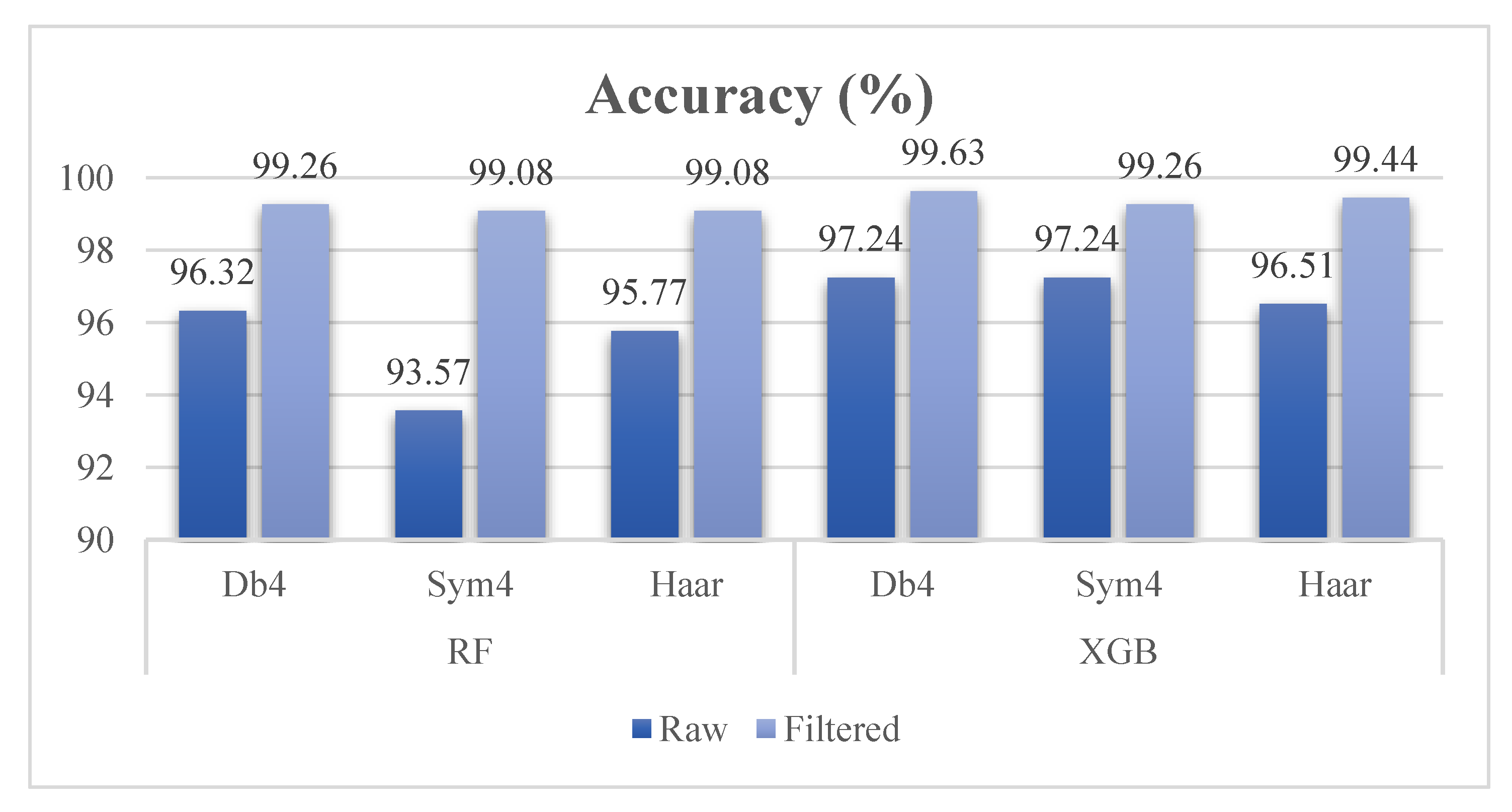
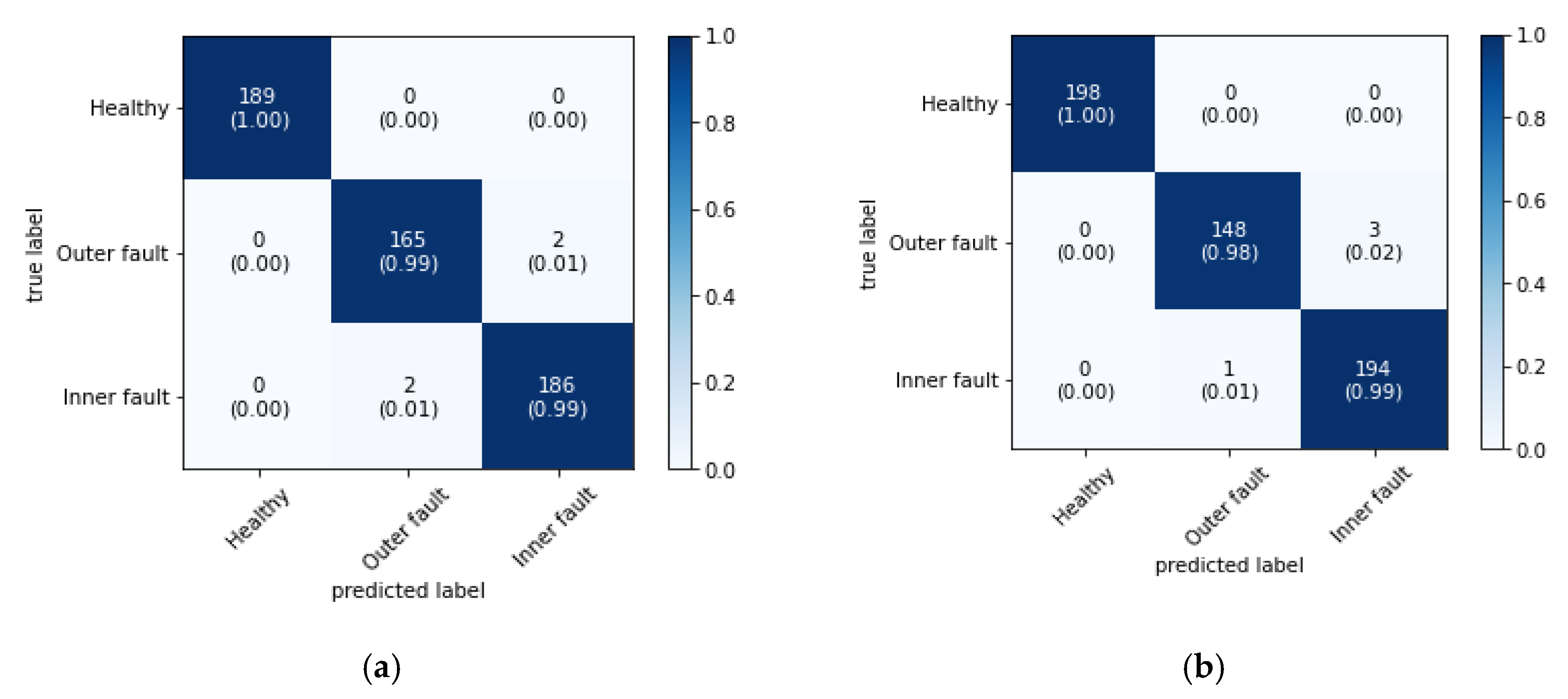
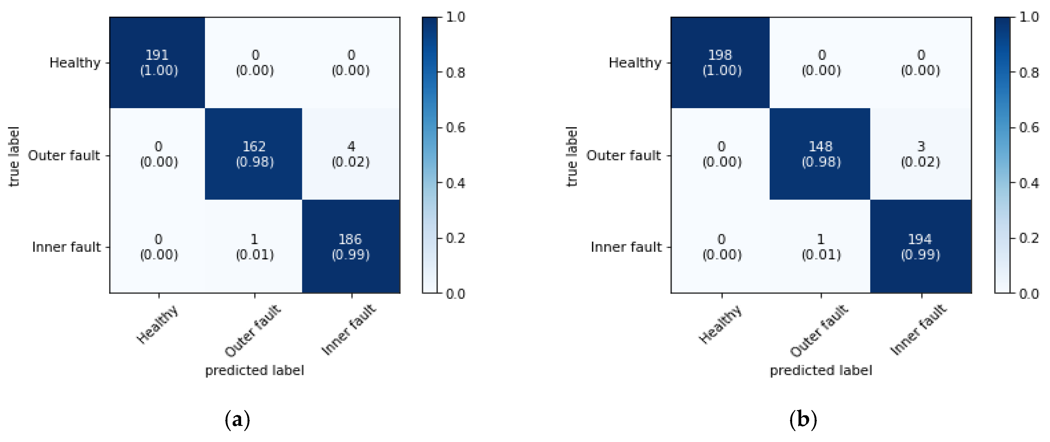
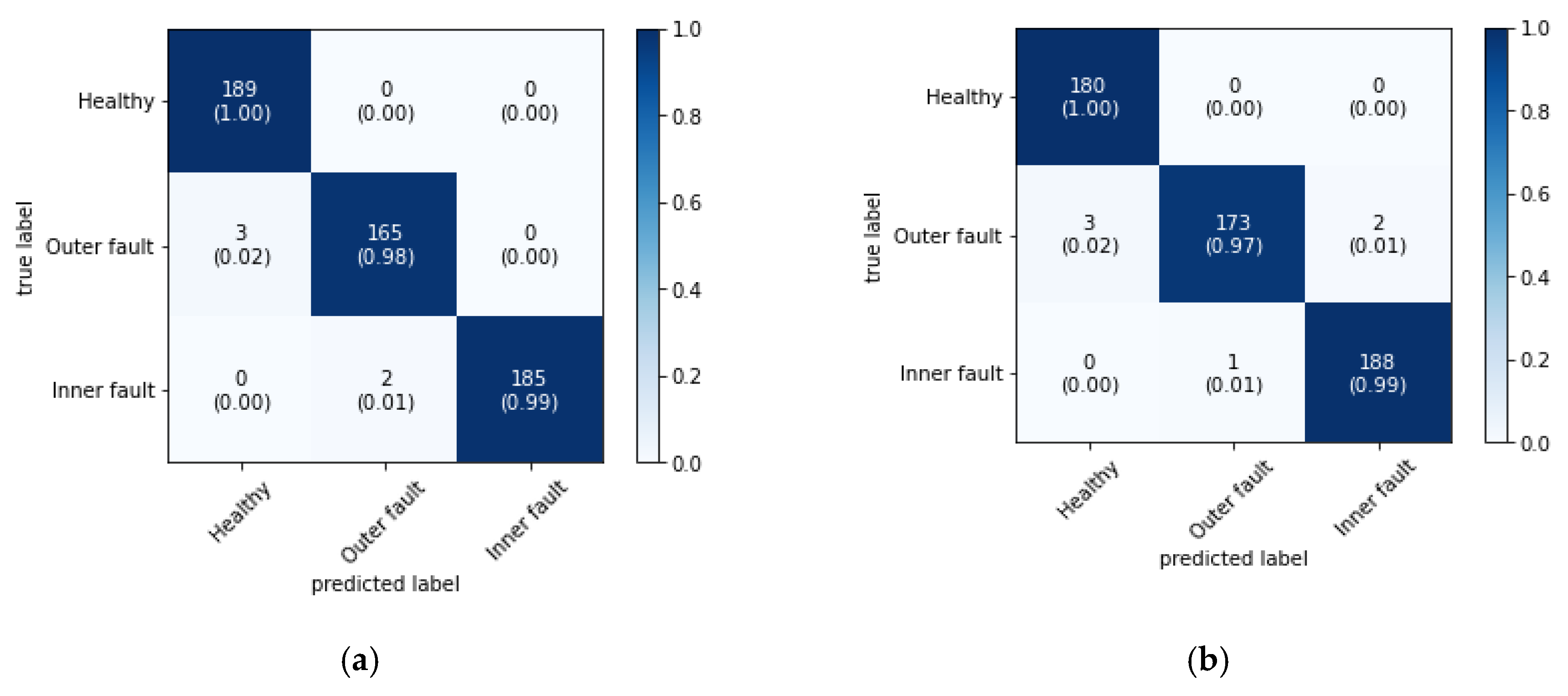
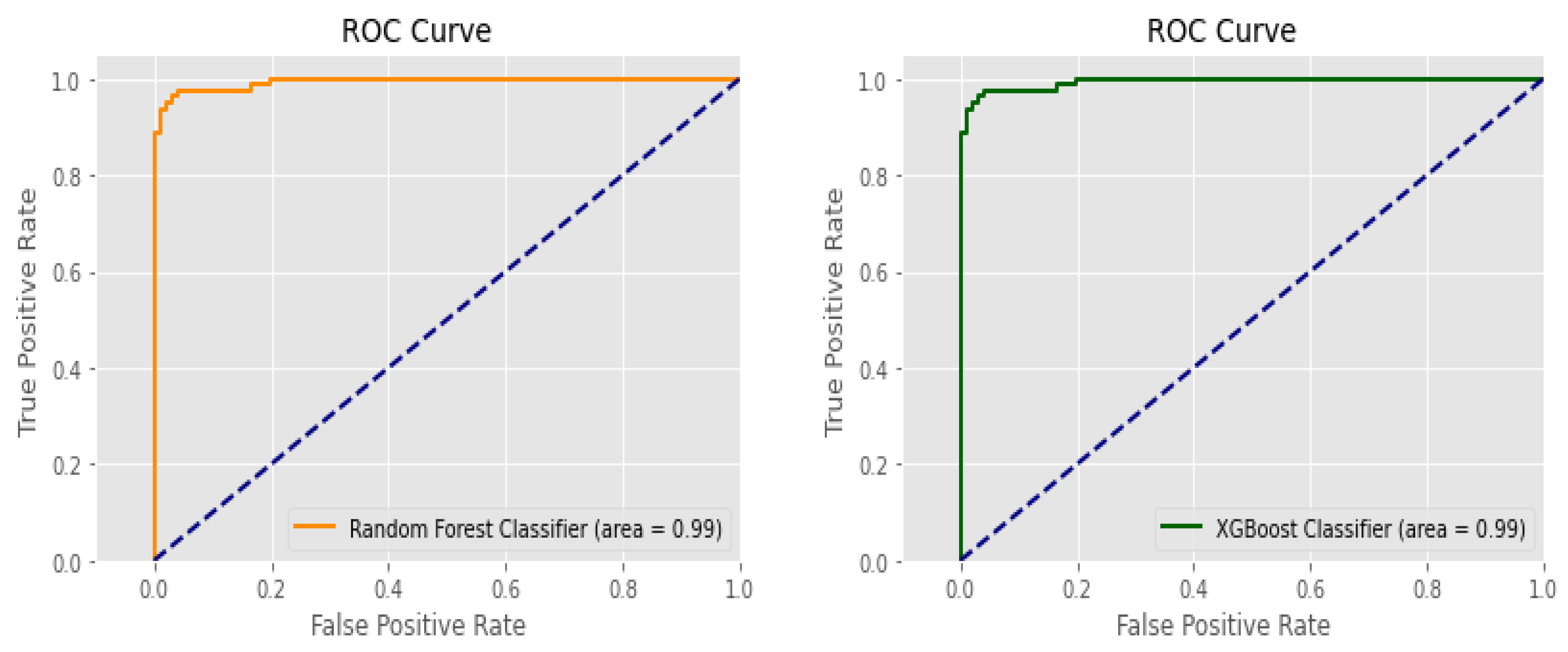
The optimal hyperparameters are determined through a process called hyperparameter search. The appropriate values of the hyperparameters increases the accuracy of the training model. In order to finding the set of optimal hyperparameters, each independent set is applied by k-fold cross-validation and finally, the most appropriate set of hyperparameters is determined by applying “GridSearchCV”, which a scikit-learn class. For both classifiers, a broad range of parameters was tested. The optimum parameters found after the GridSearch method for two ensemble learning are listed in

Table 5. Optimum parameters.

Random Forest		Xtreme Gradient Boosting
Parameters	Values	Parameters	Values
max_depth	90	max_depth	20
max_features	3	learning rate	0.1
min_samples_leaf	3	n_estimator	500
min_samples_split	8	min_child_weight	1
n_estimators	200	gamma	1

. Also, we applied 5-fold cross validation to enhance reliability of the output.

Finally, with the optimum parameters of the classifiers, the feature matrix was split into training and testing subsets with 80:20 ratio for training and validation of the fault classification abilities for the RF and XGBoost classification algorithms.

4. Results

After selecting the hyperparameter values, the two classifiers are trained. The training and test ratios were chosen as 80:20. A 5-fold cross-validation approach was utilized to validate the trained models. The overall process was carried out with the non-filtered data, and the parameters mentioned in Equations (23)–(27) were determined, as provided in

Table 6. The five evaluation parameters of two classifiers for three wavelets executed on the raw signal.

	RF			XGB
	db4	Sym4	Haar	db4	Sym4	Haar
Precision	0.96	0.94	0.96	0.97	0.97	0.97
Sensitivity	0.96	0.94	0.96	0.97	0.97	0.97
F1_score	0.96	0.94	0.96	0.97	0.97	0.97
Specificity	0.96	0.94	0.96	0.97	0.97	0.97
Accuracy	0.96	0.93	0.95	0.97	0.97	0.96

.

In the next step, the filtered signal from a notch filter is obtained, and the process is repeated. In this approach with the filtered signal, greater than 99% accuracy was achieved for both classifiers. The performance evaluation parameters for the filtered signal are listed in

Table 7. The five evaluation parameters of two classifiers for three wavelets executed on the filtered signal.

	RF			XGB
	db4	Sym4	Haar	db4	Sym4	Haar
Precision	0.99	0.99	0.99	0.99	0.99	0.99
Sensitivity	0.99	0.99	0.99	1.0	0.99	0.99
F1_score	0.99	0.99	0.99	1.0	0.99	1.0
Specificity	0.99	0.99	0.99	0.99	0.99	0.99
Accuracy	0.99	0.99	0.99	0.99	0.99	0.99

for the two ensemble classifiers.

The bar chart in Figure 12 indicates the improvement in accuracy after filtering the current signal.

The corresponding confusion matrices are presented in Figure 13, Figure 14 and Figure 15. From the confusion matrices, it is evident that the classifiers are very successfully classifying the faults, as the false positive and the false negative numbers are negligible. Also, in the ROC, the area under the curve is provided in Figure 16 and ensures that the models can distinguish among the classes.

Finally,

Table 8. Comparison of classification accuracy among the various methods.

Applied Methodology	Classification Accuracy (%)
WPD + SVM-PSO [50]	86.03
IF+MLP [51]	98.3
SVM+ IF [51]	98.0
KNN+ IF [51]	97.7
CNN + EWT [52]	97.3
DWT + XGBoost [This paper]	99.3

presents a comparison of the other models investigated with the same dataset in different works. Wavelet packet decomposition up to three levels, along with the special SVM approach named SVM-PSO (SVM—particle swarm optimization), was implemented by Lessmeier et al. [50] and achieved an accuracy of 86.03%. Information fusion (IF) and DL approaches were used [51] on a motor current signal, which result almost 98.3% accuracy. Another study on the same dataset applied an empirical wavelet transform and CNN for fault classification, showing 97.37% accuracy [52]. Therefore, by comparison with the recent research on the motor current signal, our approach provides a better result, with greater than 99% accuracy for ensemble classifiers.

5. Conclusions

In recent times, the complexity of the modern industrial system continues to advance because the multi-sensor network has become an essential component in comprehensive systems. Electrical current analysis has emerged as an intelligent solution that simplifies the fault diagnosis process with a small number of sensors. Therefore, the cost is reduced by featuring sensor less and extensive technologies. In this study, a data-driven approach using a motor current signal analyzed by DWT and ensemble machine learning methods was proposed for IM bearing fault diagnosis. The three mother wavelets of db4, sym4, and Haar were applied for signal decomposition. Both raw and filtered signals were used separately as input of wavelet decomposition. Though we performed a high-level decomposition, high and low frequency component properties showed equal importance. The feature set was constructed from the detailed and approximation coefficients, which act as the input of the two ensemble classifiers. Here, the two phased currents of three conditions of the IM bearing were considered. The purpose of this study was to not only attain high accuracy, but also reduce power and computational complexity by eliminating redundant data. Both RF and grid search classifiers achieved greater than 99% accuracy for all three wavelets on the filtered signal, and other evaluation parameters also outperformed. The time frequency domain-based feature extraction was efficient, with very high accuracy and no feature selection. Finally, a comparison with some recent works is presented and indicates that the wavelet decomposition techniques with the ML ensemble classifier algorithms can be a promising model for bearing fault classification.

References

1. Khan, S.; Yairi, T. A review on the application of deep learning in system health management. Mech. Syst. Signal Process. 2018, 107, 241–265. [Google Scholar] [CrossRef]
2. Liao, Y.X.; Zhang, L.; Li, W.H. Regrouping particle swarm optimization based variable neural network for gearbox fault diagnosis. J. Intell. Fuzzy Syst. 2018, 34, 3671–3680. [Google Scholar] [CrossRef]
3. Zhao, R.; Yan, R.Q.; Chen, Z.H.; Mao, K.Z.; Wang, P.; Gao, R.X. Deep learning and its applications to machine health monitoring. Mech. Syst. Signal Process. 2019, 115, 213–237. [Google Scholar] [CrossRef]
4. Thorsen, O.V.; Dalva, M. A survey of faults on induction-motors in offshore oil industry, petrochemical industry, gas terminals, and oil refineries. IEEE Trans. Ind. Appl. 1995, 31, 1186–1196. [Google Scholar] [CrossRef]
5. Wang, D.; Miao, Q.; Fan, X.F.; Huang, H.Z. Rolling element bearing fault detection using an improved combination of Hilbert and Wavelet transforms. J. Mech. Sci. Technol. 2009, 23, 3292–3301. [Google Scholar] [CrossRef]
6. Patil, A.B.; Gaikwad, J.A.; Kulkarni, J.V. Bearing fault diagnosis using discrete wavelet transform and artificial neural network. In Proceedings of the 2016 2nd International Conference on Applied and Theoretical Computing and Communication Technology (iCATccT), Bangalore, India, 21–23 July 2016; pp. 399–405. [Google Scholar]
7. Lee, J.H.; Pack, J.H.; Lee, I.S. Fault diagnosis of induction motor using convolutional neural network. Appl. Sci. 2019, 9, 2950. [Google Scholar] [CrossRef] [Green Version]
8. Glowacz, A. Acoustic based fault diagnosis of three-phase induction motor. Appl. Acoust. 2018, 137, 82–89. [Google Scholar] [CrossRef]
9. Liu, J.; Shao, Y.M. Overview of dynamic modelling and analysis of rolling element bearings with localized and distributed faults. Nonlinear Dyn. 2018, 93, 1765–1798. [Google Scholar] [CrossRef]
10. Immovilli, F.; Bianchini, C.; Cocconcelli, M.; Bellini, A.; Rubini, R. Bearing Fault model for induction motor with externally induced vibration. IEEE Trans. Ind. Electron. 2013, 60, 3408–3418. [Google Scholar] [CrossRef]
11. Sohaib, M.; Kim, C.H.; Kim, J.M. A hybrid feature model and deep-learning-based bearing fault diagnosis. Sensors 2017, 17, 2876. [Google Scholar] [CrossRef] [Green Version]
12. Elbouchikhi, E.; Choqueuse, V.; Auger, F.; Benbouzid, M.E. Motor current signal analysis based on a matched subspace detector. IEEE Trans. Instrum. Meas. 2017, 66, 3260–3270. [Google Scholar] [CrossRef] [Green Version]
13. Soualhi, A.; Clerc, G.; Razik, H. Detection and diagnosis of faults in induction motor using an improved artificial ant clustering technique. IEEE Trans. Ind. Electron. 2013, 60, 4053–4062. [Google Scholar] [CrossRef]
14. Zhou, W.; Habetler, T.G.; Harley, R.G. Bearing fault detection via stator current noise cancellation and statistical control. IEEE Trans. Ind. Electron. 2008, 55, 4260–4269. [Google Scholar] [CrossRef]
15. Ince, T.; Kiranyaz, S.; Eren, L.; Askar, M.; Gabbouj, M. Real-time motor fault detection by 1-D Convolutional neural networks. IEEE Trans. Ind. Electron. 2016, 63, 7067–7075. [Google Scholar] [CrossRef]
16. Pons-Llinares, J.; Antonino-Daviu, J.A.; Riera-Guasp, M.; Lee, S.B.; Kang, T.J.; Yang, C. Advanced Induction motor rotor fault diagnosis via continuous and discrete time-frequency tools. IEEE Trans. Ind. Electron. 2015, 62, 1791–1802. [Google Scholar] [CrossRef]
17. Zhen, D.; Wang, Z.L.; Li, H.Y.; Zhang, H.; Yang, J.; Gu, F.S. An improved cyclic modulation spectral analysis based on the CWT and its application on broken rotor bar fault diagnosis for induction motors. Appl. Sci. 2019, 9, 3902. [Google Scholar] [CrossRef] [Green Version]
18. Sinha, J.K.; Elbhbah, K. A future possibility of vibration based condition monitoring of rotating machines. Mech. Syst. Signal Process. 2013, 34, 231–240. [Google Scholar] [CrossRef]
19. Antoni, J. Cyclic spectral analysis of rolling-element bearing signals: Facts and fictions. J. Sound Vib. 2007, 304, 497–529. [Google Scholar] [CrossRef]
20. Parey, A.; El Badaoui, M.; Guillet, F.; Tandon, N. Dynamic modelling of spur gear pair and application of empirical mode decomposition-based statistical analysis for early detection of localized tooth defect. J. Sound Vib. 2006, 294, 547–561. [Google Scholar] [CrossRef]
21. He, Q.B.; Wang, X.X. Time-frequency manifold correlation matching for periodic fault identification in rotating machines. J. Sound Vib. 2013, 332, 2611–2626. [Google Scholar] [CrossRef]
22. Li, Z.; Feng, Z.P.; Chu, F.L. A load identification method based on wavelet multi-resolution analysis. J. Sound Vib. 2014, 333, 381–391. [Google Scholar] [CrossRef]
23. Pothisarn, C.; Klomjit, J.; Ngaopitakkul, A.; Jettanasen, C.; Asfani, D.A.; Negara, I.M.Y. Comparison of various mother wavelets for fault classification in electrical systems. Appl. Sci. 2020, 10, 1203. [Google Scholar] [CrossRef] [Green Version]
24. Peng, Z.K.; Tse, P.W.; Chu, F.L. An improved Hilbert–Huang transform and its application in vibration signal analysis. J. Sound Vib. 2005, 286, 187–205. [Google Scholar] [CrossRef]
25. Liu, X.F.; Bo, L.; He, X.X.; Veidt, M. Application of correlation matching for automatic bearing fault diagnosis. J. Sound Vib. 2012, 331, 5838–5852. [Google Scholar] [CrossRef]
26. Kar, C.; Mohanty, A.R. Vibration and current transient monitoring for gearbox fault detection using multiresolution Fourier transform. J. Sound Vib. 2008, 311, 109–132. [Google Scholar] [CrossRef]
27. Lu, W.B.; Jiang, W.K.; Yuan, G.Q.; Yan, L. A gearbox fault diagnosis scheme based on near-field acoustic holography and spatial distribution features of sound field. J. Sound Vib. 2013, 332, 2593–2610. [Google Scholar] [CrossRef]
28. Li, B.; Chen, X.F.; Ma, J.X.; He, Z.J. Detection of crack location and size in structures using wavelet finite element methods. J. Sound Vib. 2005, 285, 767–782. [Google Scholar] [CrossRef]
29. Nikravesh, S.; Chegini, S.N. Crack identification in double-cracked plates using wavelet analysis. Meccanica 2013, 48, 2075–2098. [Google Scholar] [CrossRef]
30. Chen, J.L.; Pan, J.; Li, Z.P.; Zi, Y.Y.; Chen, X.F. Generator bearing fault diagnosis for wind turbine via empirical wavelet transform using measured vibration signals. Renew. Energy 2016, 89, 80–92. [Google Scholar] [CrossRef]
31. Muralidharan, V.; Sugumaran, V. Feature extraction using wavelets and classification through decision tree algorithm for fault diagnosis of mono-block centrifugal pump. Measurement 2013, 46, 353–359. [Google Scholar] [CrossRef]
32. Zimroz, R.; Bartelmus, W.; Barszcz, T.; Urbanek, J. Diagnostics of bearings in presence of strong operating conditions non-stationarity—A procedure of load-dependent features processing with application to wind turbine bearings. Mech. Syst. Signal Process. 2014, 46, 16–27. [Google Scholar] [CrossRef]
33. Adly, A.R.; El Sehiemy, R.A.; Abdelaziz, A.Y.; Ayad, N.M.A. Critical aspects on wavelet transforms based fault identification procedures in HV transmission line. IET Gener. Transm. Dis. 2016, 10, 508–517. [Google Scholar] [CrossRef]
34. Gangsar, P.; Tiwari, R. A support vector machine based fault diagnostics of Induction motors for practical situation of multi-sensor limited data case. Measurement 2019, 135, 694–711. [Google Scholar] [CrossRef]
35. Pandhare, V.; Singh, J.; Lee, J. Convolutional neural network based rolling-element bearing fault diagnosis for naturally occurring and progressing defects using time-frequency domain features. In Proceedings of the Prognostics and System Health Management Conference (PHM-Paris), Paris, France, 2–5 May 2019. [Google Scholar]
36. Liu, R.N.; Yang, B.Y.; Zhang, X.L.; Wang, S.B.; Chen, X.F. Time-frequency atoms-driven support vector machine method for bearings incipient fault diagnosis. Mech. Syst. Signal Process. 2016, 75, 345–370. [Google Scholar] [CrossRef]
37. Moosavian, A.; Jafari, S.M.; Khazaee, M.; Ahmadi, H. A comparison between ANN, SVM and least squares SVM: Application in multi-fault diagnosis of rolling element bearing. Int. J. Acoust. Vib. 2018, 23, 432–440. [Google Scholar] [CrossRef]
38. Shao, H.D.; Jiang, H.K.; Li, X.Q.; Wu, S.P. Intelligent fault diagnosis of rolling bearing using deep wavelet auto-encoder with extreme learning machine. Knowl. Based Syst. 2018, 140, 1–14. [Google Scholar] [CrossRef]
39. Chen, Z.Y.; Li, W.H. Multisensor feature fusion for bearing fault diagnosis using sparse autoencoder and deep belief network. IEEE Trans. Instrum. Meas. 2017, 66, 1693–1702. [Google Scholar] [CrossRef]
40. Huang, R.Y.; Liao, Y.X.; Zhang, S.H.; Li, W.H. Deep decoupling convolutional neural network for intelligent compound fault diagnosis. IEEE Access 2019, 7, 1848–1858. [Google Scholar] [CrossRef]
41. Jia, F.; Lei, Y.G.; Guo, L.; Lin, J.; Xing, S.B. A neural network constructed by deep learning technique and its application to intelligent fault diagnosis of machines. Neurocomputing 2018, 272, 619–628. [Google Scholar] [CrossRef]
42. Shao, H.D.; Jiang, H.K.; Zhang, H.Z.; Duan, W.J.; Liang, T.C.; Wu, S.P. Rolling bearing fault feature learning using improved convolutional deep belief network with compressed sensing. Mech. Syst. Signal Process. 2018, 100, 743–765. [Google Scholar] [CrossRef]
43. Divina, F.; Gilson, A.; Gomez-Vela, F.; Torres, M.G.; Torres, J.E. Stacking ensemble learning for short-term electricity consumption forecasting. Energies 2018, 11, 949. [Google Scholar] [CrossRef] [Green Version]
44. Zhang, C.; Ma, Y. (Eds.) Ensemble Machine Learning: Methods and Applications; Springer Science & Business Media: Boston, MA, USA, 2012. [Google Scholar]
45. Breiman, L. Random forests. Mach. Learn. 2001, 45, 5–32. [Google Scholar] [CrossRef] [Green Version]
46. Chen, T.; Guestrin, C. Xgboost: A scalable tree boosting system. In Proceedings of the 22nd Acm Sigkdd International Conference on Knowledge Discovery and Data Mining ACM, San Francisco, CA, USA, 13–17 August 2016; pp. 785–794. [Google Scholar]
47. Chakraborty, D.; Elzarka, H. Early detection of faults in HVAC systems using an XGBoost model with a dynamic threshold. Energy Build. 2019, 185, 326–344. [Google Scholar] [CrossRef]
48. Zhang, D.H.; Qian, L.Y.; Mao, B.J.; Huang, C.; Huang, B.; Si, Y.L. A data-driven design for fault detection of wind turbines using random forests and XGboost. IEEE Access 2018, 6, 21020–21031. [Google Scholar] [CrossRef]
49. Zhang, R.; Li, B.; Jiao, B. Application of XGboost algorithm in bearing fault diagnosis. In IOP Conference Series: Materials Science and Engineering, Proceedings of the 2nd International Symposium on Application of Materials Science and Energy Materials (SAMSE 2018), Shanghai, China, 17–18 December 2018; IOP Publishing: Bristol, UK, 2019; Volume 490. [Google Scholar] [CrossRef]
50. Lessmeier, C.K.; Kimotho, J.K.; Zimmer, D.; Sextro, W. Condition monitoring of bearing damage in electromechanical drive systems by using motor current signals of electric motors: A benchmark data set for data-driven classification. In Proceedings of the European Conference of the Prognostics and Health Management Society, Bilbao, Spain, 5–8 July 2016; 2016. [Google Scholar]
51. Hoang, D.T.; Kang, H.J. A motor current signal-based bearing fault diagnosis using deep learning and information fusion. IEEE Trans. Instrum. Meas. 2020, 69, 3325–3333. [Google Scholar] [CrossRef]
52. Hsueh, Y.M.; Ittangihal, V.R.; Wu, W.B.; Chang, H.C.; Kuo, C.C. Fault diagnosis system for induction motors by CNN using empirical wavelet transform. Symmetry 2019, 11, 1212. [Google Scholar] [CrossRef] [Green Version]
53. Oswald, F.B.; Zaretsky, E.V.; Poplawski, J.V. Effect of internal clearance on load distribution and life of radially loaded ball and roller bearings. Tribol. Trans. 2012, 55, 245–265. [Google Scholar] [CrossRef]
54. Bloedt, M.; Granjon, P.; Raison, B.; Rostaing, G. Models for bearing damage detection in induction motors using stator current monitoring. IEEE Trans. Ind. Electron. 2008, 55, 1813–1822. [Google Scholar] [CrossRef] [Green Version]
55. Jung, J.H.; Lee, J.J.; Kwon, B.H. Online diagnosis of induction motors using MCSA. IEEE Trans. Ind. Electron. 2006, 53, 1842–1852. [Google Scholar] [CrossRef]
56. Nikravesh, S.Y.; Rezaie, H.; Kilpatrik, M.; Taheri, H. Intelligent fault diagnosis of bearings based on energy levels in frequency bands using wavelet and Support Vector Machines (SVM). J. Manuf. Mater. Process. 2019, 3, 11. [Google Scholar] [CrossRef] [Green Version]
57. Wu, J.D.; Chen, J.C. Continuous wavelet transform technique for fault signal diagnosis of internal combustion engines. NDT E Int. 2006, 39, 304–311. [Google Scholar] [CrossRef]
58. Eristi, H.; Ucar, A.; Demir, Y. Wavelet-based feature extraction and selection for classification of power system disturbances using support vector machines. Electr. Power Syst. Res. 2010, 80, 743–752. [Google Scholar] [CrossRef]
59. Maritnez-Alvarez, F.; Troncoso, A.; Asencio-Cortes, G.; Riquelme, J.C. A survey on data mining techniques applied to electricity-related time series forecasting. Energies 2015, 8, 13162–13193. [Google Scholar] [CrossRef] [Green Version]
60. Chakraborty, D.; Elzarka, H. Advanced machine learning techniques for building performance simulation: A comparative analysis. J. Build. Perform. Simul. 2019, 12, 193–207. [Google Scholar] [CrossRef]
Figure 1. Organization of the test rig.
Applsci 10 05251 g001
Figure 2. Time domain signal of different bearing conditions.
Applsci 10 05251 g002
Figure 3. Frequency domain representation of different bearing conditions.
Applsci 10 05251 g003
Figure 4. Workflow of the proposed method for bearing fault classification of IM.
Applsci 10 05251 g004
Figure 5. (a) Structure of a rolling-element bearing; (b) Outer race defect; (c) Inner race defect.
Applsci 10 05251 g005
Figure 6. Characteristic signals of three mother wavelets.
Applsci 10 05251 g006
Figure 7. (a) Raw and (b) filtered signals of three types of bearing states.
Applsci 10 05251 g007
Figure 8. Wavelet decomposition of the ‘Haar’ mother wavelet of a healthy bearing.
Applsci 10 05251 g008
Figure 9. Wavelet decomposition of the ‘db4′ mother wavelet of the outer fault bearing.
Applsci 10 05251 g009
Figure 10. Wavelet decomposition of the ‘sym4′ mother wavelet of the inner fault bearing.
Applsci 10 05251 g010
Figure 11. (a) Random forest and (b) XGBoost algorithm architectures.
Applsci 10 05251 g011
Figure 12. Accuracy for RF and XGB for raw and filtered motor current signals.
Applsci 10 05251 g012
Figure 13. Confusion matrix of the db4 wavelet for (a) RF and (b) XGBoost classifiers.
Applsci 10 05251 g013
Figure 14. Confusion matrix of the sym4 wavelet for (a) RF and (b) XGBoost classifiers.
Applsci 10 05251 g014
Figure 15. Confusion matrix of the Haar wavelet for (a) RF and (b) XGBoost classifiers.
Applsci 10 05251 g015
Figure 16. ROC curves for the RF and XGBoost classifiers.
Applsci 10 05251 g016