Abstract
We present a complete, fully automatic solution based on genetic algorithms for the optimization of discrete product placement and of order picking routes in a warehouse. The solution takes as input the warehouse structure and the list of orders and returns the optimized product placement, which minimizes the sum of the order picking times. The order picking routes are optimized mostly by genetic algorithms with multi-parent crossover operator, but for some cases also permutations and local search methods can be used. The product placement is optimized by another genetic algorithm, where the sum of the lengths of the optimized order picking routes is used as the cost of the given product placement. We present several ideas, which improve and accelerate the optimization, as the proper number of parents in crossover, the caching procedure, multiple restart and order grouping. In the presented experiments, in comparison with the random product placement and random product picking order, the optimization of order picking routes allowed the decrease of the total order picking times to 54%, optimization of product placement with the basic version of the method allowed to reduce that time to 26% and optimization of product placement with the methods with the improvements, as multiple restart and multi-parent crossover to 21%.
1. Introduction
A large share of operating costs related to product storage is connected to order picking. Based on many studies, it has been established that about 60% of warehouse operation costs are the costs of picking up goods when completing orders [1]. As the speed of this operation is a decisive factor in the response time to customers’ orders and is one of the factors contributing to their decision about choosing or not the same company at the next purchase, it seems that the role of the speed of order completion is even greater.
Thus, shortening the time of order picking is the most important and most beneficial factor in reducing the costs of operating the warehouse. It can be achieved without significant costs by optimizing the locations for particular products in a warehouse and then determining the fastest order completion routes in the optimized product placement.
Some aspects of the optimization seems obvious, for example that items that are often ordered together should be placed close to each other, and frequently purchased items should be located close to the delivery point. However, for the case of discrete variables, considered in this paper, where the location sizes are fixed (some goods, e.g., storage of the sand, gravel, and so forth, can be expressed by continuous variables, but this problem is not considered here), with N items in the warehouse, the number of all possible their placements is . For it gives , and even if the computer could analyze 1 billion permutations per second, it would years to find the best product placement. So in practice, designing manually an optimal product placement is impossible, as the number of possible arrangements significantly exceeds the possibilities of analyzing all solutions by humans, or even by a computer program, which tries all possible configurations.
In this paper, we present a complete, fully automated system based on artificial intelligence, particularly on genetic algorithms, which can overcome the limitations of the search space by an intelligent search. The system usually analyzes only several thousands to several tens of thousands possible product placements to find the optimal solution or at least a solution so close to the optimal one, that in practice it will not make any difference. Moreover, the system returns also the quickest order picking routes. The advantage of applying such a solution is speeding up the operations and thus reduction of warehouse operating costs (where typically 60% are the costs of order picking [1]) and the possibility to serve more customers by the same employees in the same time and thus to further increase the sales and profits.
Although this issue has been analyzed for a long time, and especially in recent years its intensive development has been taking place [2,3,4], we were not able to find in the literature a complete, accurate, fully automatic solution, which would consider the real distribution of orders in the optimization of product placements. All the papers we were able to find presented only some partial approaches, with big simplifications, for example that the route length is determined only by one product with the longest distance from the entrance [2], or that the user is responsible for re-allocating the products by placing the more frequently used closer to the entrance [5].
Moreover, frequently the list of products within a single order is quite long, especially in the warehouses which sell goods mostly to retailers, what makes the optimization even more important. The purpose of this paper is to fill the gap by presenting our solution and by discussing its particular aspects and their influence on the accuracy and speed of the warehouse optimization process.
First we define the problem (Section 2), then we list the main points of our contribution (Section 3), next we come to the details in the following order: the literature review (Section 4), presentation of the proposed solution (Section 5.1, Section 5.2, Section 5.3 and Section 5.4), experimental results (Section 6) and conclusions (Section 7).
2. Problem Statement
The product placement determines the locations (usually shelves) of particular products in the warehouse. We define the cost of a product placement as the sum of the shortest order picking routes over all orders included in the order list for this product placement (Equation (1)). The assumption behind that is that if robots are used to collect the orders, then they will exactly follow the shortest routes found. If humans pick the orders, they will in most cases follow the same routes, however, sometimes they may decide to change the path. This can be however treated as random process and thus cannot be taken into account in the optimization.
where is the number orders in the order list and is the shortest order picking (order completion) route found for the n-th order.
The problem to solve is to find a product placement with with as low cost as possible. In other words we need to minimize the cost given by Equation (1) by proper products placing at particular locations in a warehouse.
For that purpose we developed the product placement optimization algorithm, which we describe in the following sections.
The inputs to the algorithm are:
- warehouse layout in the form of transition costs between neighboring locations
- the list of orders
The outputs of the algorithm are:
- the optimized product placement in the warehouse
- shortest order picking routes for each order from the order list for the optimized product placement
Here we only present the main idea and the details about each input and output can be found in the subsequent sections. The order list contains all considered orders, which should be the orders expected in a certain future period of time. In most cases these can be the past orders, as we can expect that the future orders will have the same distribution of products. Otherwise these can be the past orders from a corresponding season of the last year or the predicted future orders. Each order consists of several (at least one) products. To complete the order, the locations of all the products that are included in the order must be visited and the products must be picked. Thus a sub-problem of the main problem of product placement optimization is to find the quickest (shortest) order completion route for each order. This is necessary, as the sum of the quickest order picking routes is the main objective that we want to minimize by optimizing the placement of particular products in the warehouse.
This sub-problem of finding the quickest order completion route is equivalent to the Traveling Salesman Problem (TSP). While, the whole optimization of product placement is a different, much more complex problem. The main differences are:
- In product placement optimization, the task is to find optimal product locations. In TSP the task is to find the shortest route connecting all considered locations.
- In product placement optimization, the cost function that we use is the sum of the shortest order picking routes for a given product placement (Equation (1)). In TSP the cost function is the length a single route connecting all considered locations.
- Product placement optimization is a two-level nested task, where the main (outer) process is the product placement optimization itself and the inner process calculates the cost (fitness) of each considered product placement by finding the shortest order picking routes and then summing them to obtain the cost. TSP is a single level problem, without any nested optimization.
- In product placement optimization the methods developed especially for TSP as nearest neighbor, or HGReX crossover in genetic algorithms cannot be used in the main process, because we do not look for any route, there does not exist any sequence of locations and there is no such a concept as “go to the next location”, which the methods use.
3. Contribution
The main points of the contribution of this paper are:
- The whole system design, with nested genetic-based optimization, where the cost of product placement is expressed by the sum of order completions times (Section 5.2).
- An improved multi-parent version of the HGreX crossover for route optimization (Section 5.4.1).
- Multiple fast restart procedure to increase the accuracy with minimal growth of the optimization time (Section 5.4.3).
- Automatic selection of the order picking route calculation method to balance the optimization speed and accuracy (Section 5.3).
- Input data format in the form of transition costs between neighboring locations, what joins maximal accuracy with minimal user effort for the data preparation Section 5.1.
- Caching of fitness values (Section 5.4.2).
4. Related Works
4.1. Warehouse Planing and Operations
A lot of literature positions were devoted to warehouse operations. Van Gils et al. [4] provided a review and classification of the scientific literature investigating combinations of tactical and operational order picking planning problems. Grosse et al. [6] analyzed human factors in order picking. Dijkstra and Roodbergen [7] discussed predetermined order picking sequences, including various layouts of the warehouse and its aisles. They also discussed a dynamic programming approach that determines storage location assignments for those layouts, using the route length formulas and optimal properties. Bolaños Zuñiga [3] presented a formal mathematical model for simultaneously determining storage location assignment and picker routing, considering precedence constraints based on the weight of the products and location for each product in a general warehouse. Bartholdi [1] in his book presented practical considerations for warehouse planning and construction. Rakesh [8] discussed methods that determine optimal lane depth, number of storage levels, and other parameters of warehouse layout to minimize space and material handling costs. The book of Davarzani [9] discussed warehouse planning, technology, equipment, human resource management, connections to other department and companies. Zunic [10] considered various warehouse designs, especially the V-shape isles and calculated the order picking routes for these designs. Dharmapriya [11] discussed the use of simulated annealing for the warehouse layout optimization taking into account the total demand and traveling cost, but without considering the co-existence of various products in the same orders.
4.2. Genetic Algorithms in Warehouse Optimization
Artificial intelligence methods, in particular genetic algorithms, are solutions that have numerous successful implementations and that have been rapidly gaining popularity in recent years and were applied also to warehouse operation optimizations [12,13,14].
Genetic algorithms have two important advantages: fast intelligent search used to find the product placement and a global cost function.
Their first advantage is that due to intelligent searching, genetic algorithms do not need to analyze all solutions (all possible permutations of product locations), which is impossible due to their number. They usually analyze only a few thousands up to few hundred thousands of product placements (and not all possibilities) to find the solution. Although genetic algorithms do not guarantee finding the optimal solution every time, the solutions found are close enough to the optimal solution so that in practice this does not make a significant difference.
Their second advantage is that using genetic algorithms, we do not have to define ourselves the rules that characterize good solutions. This is a very important, because usually we do not know how to define the rules optimally, and we only have some intuitive knowledge (e.g., goods often purchased together should be close to each other). However, the expression of this knowledge in the strict mathematical form is impossible because of the complexity of the system and the frequently opposite optimums of various order completions. With genetic algorithms it is enough to formulate the cost function, which is expressed here as the sum of all order picking route lengths or as the total time required to complete all orders from a certain period.
In genetic algorithms, the problem is coded using arrays called chromosomes by analogy with encoding in the chromosomes of biological organisms [12,13]. Each product placement encoded by a chromosome represents one solution (one individual). Initially, a pool of random solutions is generated (in each solution the products are randomly assigned to the locations in a warehouse). Then an intelligent search is applied with the help of three basic operations—selection, crossover and mutation. The selection mechanism selects individuals for the crossover operator. It is organized by analogy to the biological process, where the better individuals have a higher probability of becoming parents and exchanging information to create offspring.
The crossover operator generates a new individual (child) from the existing ones (parents). In this way it allows to combine the information encoded in the chromosomes of different individuals into one new individual. The mutation mechanism exchanges the values between some positions in an individual chromosome. Then selected individuals are promoted to the next generation. The process is repeated iteratively as long as the satisfactory solution is found or as long as the improvement in the solutions is still occurring.
To sum up, it should be stated that the use of genetic algorithms or other evolutionary optimization methods in applications to warehouse systems, including the optimization of the distribution of goods and order picking routes can bring measurable benefits to companies using these solutions, accelerating their work and reducing operating costs.
Although the idea of applying genetic algorithms to warehouse optimization or order picking route optimization was presented in some literature positions, we have not found a complete automatic solution, which considers the order distribution, as we present in this paper.
As the optimization of the order picking route (which is equivalent to the traveling salesman problem— see Section 2) is a much simpler problem than the optimization of product placement in the warehouse, as it can be expected, much more papers are dedicated to the order picking route optimization and only few papers discuss the product placement optimization. Below we shortly present some of them.
Wang [5] applied genetic algorithms to optimize a fitness function consisting of three weighed terms—the turnover of goods, the gravity center of storage racks and the relevance of the goods. Wei [15] used a similar approach with genetic algorithm with PMX crossover and the fitness were defined by the terms of the aisle access, the weight of the items and the dimensions of the shelves.
Avdeikins and Savrasovs [2] applied genetic algorithms to warehouse optimization using order crossover (OX). Each individual in the population represented a warehouse layout. Each gene was a unique item. In their solution the fitness of each individual was calculated as the sum of maximal picking distance for each order—, where O was the order from the set 1, 2, …, k and was the distance to furthest picking position. Distances were expressed by an integer value that for the first item was 1, for second 2, and so forth, increasing by 1 from one SKU to another. Using such fitness function moves the most frequently sold items closer to the warehouse entry, but this does not place in neighboring locations items that are frequently sold together, as this solution did not consider this aspect, neither it determines the real order picking routes and thus this cannot be considered a complete solution.
As the solution presented by Avdeikins and Savrasovs [2] may at the first glance seem similar to our solution, it is worth pointing out the differences. In our solution the fitness is calculated as a sum of all order picking route lengths. This is a fundamental difference between their work and our solution, as this allows us to minimize the time of the real order picking operations and thus for obtaining very accurate solutions, which also minimizes the distances between items contained in one order. The next difference is, that we use real transition costs (or real distances) and not an approximation by increasing the distance always by one, as was used by them. The next difference is that our solution determines as well the product placement as the fastest order picking routes. Moreover, we use newer, effective crossover operators and propose a lot of improvements to accuracy and speed of the optimization.
4.3. Crossover Operators
Proper design of the crossover operator is a crucial factor in genetic algorithm performance. In this subsection we review the crossover operators and present in detail the AEX and HGreX operators, which are used in our solution.
Crossover allows to combine together the most valuable information from two or more different chromosomes (parents) into one chromosome (child) that can represent a better solution than its parents. For that kind of problems, where each item can occupy only one location at a time and each location must be occupied by one item, as order picking route optimization or product placement optimization in a warehouse, special crossover operators must be used to ensure that there will be no duplicate elements and that each element will be present in the newly created individual. Several such crossover operators have been developed.
Hassanat and Alkafaween [16] proposed several crossover operators, such as cut on worst gene crossover (COWGC) and collision crossover, and selection approaches, as select the best crossover (SBC). COWGC exchanges genes between parents by cutting the chromosome at the point that maximally decreases the cost. The collision crossover uses two selection strategies for the crossover operators. The first one selects this crossover operator from several examined operators, which maximally improves the fitness and the other one randomly selects any operator. The SBC algorithm applies multiple crossover operators at the same time on the same parents, and finally selects the best two offspring to enter the population. Hwang presented the order crossover (OX) and cycle crossover (CX) operators [17]. Tan proposed heuristic greedy crossover (HGreX) and its variants HRndX and RProX [18]. Other popular crossover operators comprise partially mapped crossover (PMX) edge recombination crossover (ERX) and alternating edges crossover (ERX) [19].
Several comparisons of the performance of these crossover operators can be found in the literature [19]. Based on these comparisons, the best performing methods for the traveling salesman problem were most frequently the variants of the HGreX crossover operator and the second best was the AEX crossover operator. For this reason we decided to start our approach from applying these two crossover operators for our warehouse optimization problem.
HGreX is only suitable for those kinds of problems, where the cost of transition between two positions can be defined. For example, it can be used to find the shortest order picking path, as we can define the distances (costs) between particular locations that contain the products from the orders and thus must be visited. However, it cannot be applied to optimization of the product placement in the warehouse, because the distribution of products is not directly related to any single order picking route, but to a whole set of different routes. Thus in this case, we can define the global goal, which is the minimization of sum of the lengths of all order picking routes, but we cannot express the cost between any two positions. AEX on the other hand does not use the transition cost and therefore can be applied also to the problems, where such cost cannot be defined, as the product placement optimization in a warehouse. First we will present the AEX operator and then the HGreX operator.
AEX creates the child from two parents by starting from the value, which is at the first position in the first parent. Then it adds this value, from the second parent, which in the second parent follows the value just taken from the first parent. Then again a value from the first parent that follows the value just selected from the second parent and so one. If this is impossible, because some element would repeat, then a random not selected so far element is chosen. In the presented example each position in the chromosome represents one location in the warehouse and each letter represents one product.
Let us assume we have two parents P1 and P2:
- P1 = [ A B C D E F G H ]
- P2 = [ H A D B G F E C ]
To create the child, We start from any position of the first parent P1. Let us start from A. Then we add this value which is in the second parent after A, so we add D
- Ch = [ A D _ _ _ _ _ _ ]
- and the values remaining in the parents:
- P1 = [ B C E F G H ]
- P2 = [ H B G F E C ]
Next we add to the child this value, which is in P1 after D, that is E
- Ch = [ A D E _ _ _ _ _ ]
- and the values remaining in the parents:
- P1 = [ B C F G H ]
- P2 = [ H B G F C ]
Next we add to the child this value, which is in P2 after E, that is C
- Ch = [ A D E C _ _ _ _ ]
- and the values remaining in the parents:
- P1 = [ B F G H ]
- P2 = [ H B G F ]
Next we add to the child this value, which is in P1 after C, that is D. However, D has already been used, so this is not a valid choice. In such a case we select randomly one of the remaining values in P1. Let us select G.
- Ch = [ A D E C G _ _ _ ]
- P1 = [ B F H ]
- P2 = [ H B F ]
Next we add to the child this value, which is in P2 after G, that is F
- Ch = [ A D E C G F _ _ ]
- and the values remaining in the parents:
- P1 = [ B H ]
- P2 = [ H B ]
Next we add to the child this value, which is in P1 after F, that is currently H
- Ch = [ A D E C G F H _ ]
- and the values remaining in the parents:
- P1 = [ B ]
- P2 = [ B ]
And finally we add to the child this value, which is in P2 after H, that is currently B and the child becomes:
- Ch = [ A D E C G F H B ]
The HGreX crossover operator works in similar way to AEX. The difference is, that it does not take alternatively the elements from both parents, but always chooses this element from the two parents to which the distance (cost) from the current element is shorter (lower).
Let us assume we have the same two parents P1 and P2:
- P1 = [ A B C D E F G H ]
- P2 = [ H A D B G F E C ]
To create the child, we start from any position of the first parent P1, let us start from A. Then we add this value which has lower transition cost (shorter distance) to A from the two values that appear directly after A in both parents, that is from B and D. Let us assume that the cost of going from A to B is 12, and from A to D is 15. So we choose B as the next position in the child.
- Ch = [ A B _ _ _ _ _ _ ]
- and the values remaining in the parents:
- P1 = [ C D E F G H ]
- P2 = [ H D G F E C ]
However, if the costs were—A to B: 18, and from A to D: 15, then we would have chosen D as the next position in the child. The conflicts are resolved identically as in AEX.
In Section 5.4.1 we introduce multi-parent versions of the crossover operators.
5. The Proposed Method
In this section, we describe the proposed genetic algorithm based method that optimizes the product placement and order picking routes in the warehouse. The purpose of the method, as described in Section 2, is to minimize the product placement cost given by Equation (1), this is to find such assignment of particular products to positions in the warehouse, which minimizes the sum of the shortest order picking routes over all orders from the order list. Thus, the optimization process consists of the outer procedure (main process), which is the product placement optimization (presented in Section 5.2) and the inner procedure (the sub-process), which is the order picking route optimization for each considered product placement (presented in Section 5.3).
5.1. Data Format and Problem Encoding
This subsection explains the input data format and the problem encoding in genetic algorithm chromosomes. At the end also calculation of the transition cost matrix is explained.
To determine the quality of a given product placement (see Algorithm 1), first we must find the order picking routes for each order (see Algorithm 2). To find them, we must calculate the transition cost matrix (costs of moving between each pair of locations in the warehouse), and to calculate the full matrix, the user must provide the transition costs (or distances) between the adjacent locations.
Figure 1 shows a sample layout of a very small warehouse, which we use to explain the data format and problem encoding. Of course the real warehouses, for which the methodology was created will be much larger. In this example the distances entered by user are shown with the color lines in Figure 1 and the distance matrix with these entries is shown in Table 1. As distances are symmetric (e.g., ), it is enough to fill the distances over the diagonal. The remaining distances (e.g., ) will be calculated automatically.
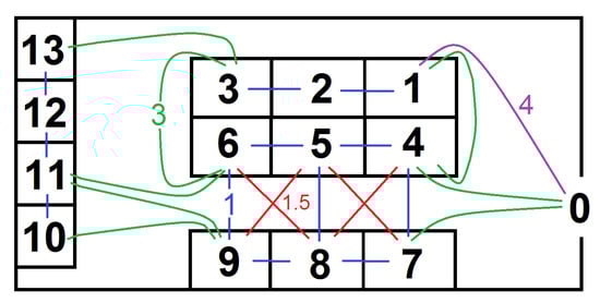
Figure 1.
Sample warehouse structure used to explain the data format and problem encoding. Distances between neighboring locations: in blue the distances of 1 unit, in red of 1.5 unit, in green of 3 units, in violet of 4 units.

Table 1.
The original distance matrix corresponding to the warehouse structure shown in Figure 1 containing only the values required by the algorithm.
The warehouse layouts with product placements and the order picking routes are encoded in the chromosomes. Let us assume that the number of available products equals the number of locations in the warehouse, that is, 13 for this sample warehouse and the products names are: A,B,C,D,E,F,G,H,I,J,K,L,M. Let us also assume that there are three different orders, which occur with the same frequency and which consist of the following products:
- Order1: A,B,C,D,E,F,G
- Order2: G,H,I,J,K
- Order3: A,B,K
For the product placement optimization we will encode the problem in a chromosome with 13 positions. At the beginning we generate a population of random individual chromosomes representing the product placements (see Algorithm 1). Let us assume, the 15th randomly generated individual looks as follows:
- Layout15 = [G H E F I J A C D K B L M]
In this case the product G is at the location 1 in Figure 1, product H at location 2, and so on. We need to find the shortest order picking routes for each individual (each product placement) to calculate its fitness. For this purpose, we generate a population of random individual chromosomes representing the routes. There is always 0 (which represents the entrance) at the first position and the other positions are occupied by randomly ordered products from this order. Let us assume, the 12th randomly generated individual for Order3 looks as follows:
- Order3-Route12 = [0 A K B 0]
The length of this route is given by the formula:
as in Layout15 is the entrance, product A at location 7, product K on location 10 and product B at location 11.
This input data format was specially designed in order to require minimal effort from the user entering the data, and at the same time to allow for maximal accuracy of calculations. Only the costs of transitions between neighboring locations are required in the input data. However, if the user wants to enter also the transition costs between some further locations, he is free to do it. The program preserves all distances entered by the user and only calculates the remaining distances.
The transition cost between locations can be entered as distance in meters, but also in seconds as the time needed to cover this distance. This takes into account that for example there is higher cost of covering the same distance vertically than horizontally or that turning around the corner requires more time than covering the same distance along a straight line and thus allowing to obtain higher accuracy of the order picking times. However, the units do not make any difference to the proposed method, which simply considers then as units of cost.
As the available plans of different warehouses can be in many different more or less usable formats, creating a separate software for preparation of the input data for each individual warehouse is no practical, as it would take more time than to enter the transition costs manually. The program does not need to know the geometrical structure of the warehouse. This is an additional advantage, because in this way much less work is required to prepare the input data.
| Algorithm 1 Product Placement (PP) Optimization Process |
| Input 1: Warehouse layout in the form of transition costs between neighboring locations (see Table 1) Input 2: The list of orders Output 1: The optimized product placement (PP) in the warehouse Output 2: Shortest order picking routes for each order for the optimized PP
|
| Algorithm 2 Order Picking Route Optimization Process |
| Input 1: The matrix of transition costs between product locations Input 2: The list of items in the j-th orders Input 3: The i-th product placement Output 1: The shortest route for the j-th order completion Output 2: The length of shortest route for the j-th order completion
|
To calculate the remaining transition costs between each pair of locations (line 1 in Algorithm 1). any algorithm that can do this can be used, for example Dijkstra [20], Floyd Warshall [21] or Bellman-Ford Algorithm [22]. We use Dijkstra Algorithm, because it is the fastest one, especially for sparse graphs (as is the case here), where each vertex is connected only with few other vertices. For a graph of v vertices (locations) and e connecting edges (transition costs), calculating all the distances with Dijkstra Algorithm with a priority queue has the complexity , while the complexity of the two other algorithms is and .
Calculating the cost matrix with the Dijkstra Algorithm takes only a very small, practically negligible, fraction of the time of the whole optimization of the product locations. Moreover, once calculated, the cost matrix can be re-used for other product placement as long as the physical layout of the warehouse does not change. The A* Algorithm [23] can be faster than Dijkstra only when the approximate cost from the current to the target node can be assessed. However, in this problem, we are not able to assess the approximate cost, because we do not know the coordinates of particular locations, but only the transition cost between neighboring locations. Considering these two factors it is not justified to demand from the user preparing additional data with coordinates of each location in order to use the A* Algorithm, as in this case the gain of the CPU time (usually less than a second) would not compensate the lost of the user’s time (usually several hours) spent on preparing the additional data.
5.2. Product Placement Optimization
In this subsection we present the algorithm used to optimize the placement of particular products in the warehouse in order to minimize the total time of completing the orders from the order list. The main optimization process is shown in pseudo-code in Algorithm 1 and as diagrams in Figure 2 and Figure 3. The sub-process, which determines the shortest order picking routes is discussed in the next section.
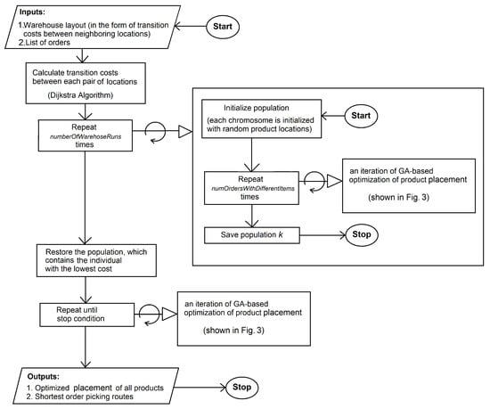
Figure 2.
Product Placement Optimization (main process).
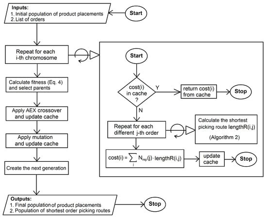
Figure 3.
Product Placement Optimization (inner block of the algorithm shown in Figure 2).
Now will explain the base version of the algorithm with (line 2 in Algorithm 1) and in Section 5.4.3 we will explain the use and purpose of multiple process restarts ().
The process starts in line 1, where the Dijkstra algorithm calculates the full matrix of transition costs (or distances) between product locations (see Section 5.1 for details). In line 3 the initial random population of product placements (PP) is generated. In line 7 the genetic algorithm starts the optimization. In line 10 the algorithm checks if any of the current individuals existed previously in current or any past epoch. If so the fitness of such an individual is not calculated but retrieved from the cache. In line 15 the shortest route for completing each different order for the current PP is calculated with Algorithm 2. Since we need to minimize the sum of order completion times, for each considered placement of products in the warehouse we need to calculate the time of each order completion and then add the times. To minimize the computational complexity of this step we group orders consisting of the same products together and assign to such an aggregated order a higher weight, which equals the number of single orders of which the aggregate order is composed. In line 18 the cost of the current PP is calculated, next the fitness is calculated from the cost and the cache is updated. In line 25 the parents for each child are selected and in the next line the child is created with the AEX crossover operator. If the fitness of the best PP has not improved for iterations (line 28) then the optimization is finished. In line 32 the promotion of children and best parents to the next generation takes place. In the next line the mutation is applied and the cache is updated. Finally in the last line the algorithm returns the best product placement and the corresponding set of the shortest order picking routes.
In order to keep the selection pressure constant and thus the exploration of the search space stronger at earlier stages and the convergence faster at later stages of the process [24] as well in product placement optimization as in the sub-process of order picking route optimization, we use use fitness function normalization. Thus the cost of a given product placement and the lengths of the order picking routes are not used directly as fitness values, but they are re-scaled. We used roulette wheel selection as well for the product placement optimization as for the order picking route optimization. According to Razali [25] and to our experiments, roulette wheel selection and tournament selection give comparable results. Also the selection pressure can be controlled in both (by number of candidates for a parent in tournament selection and by the shape of fitness function in roulette wheel selection). We chose roulette wheel selection for debugging purposes, as with this selection it was easier for to analyze the detailed algorithm behaviour and to fine-tune it.
The cost of the i-th product placement expresses the sum of the shortest routes found for each order picking and is given by Equation (2):
where is the number of different orders, is the numbers expressing how many times the j-th order is repeated on the order list and is the best (shortest) route found for the j-th order completion. The value is used to assess the progress and the results of the optimization (see Figure 3).
The fitness of the i-th product placement used by the roulette wheel selection is given by Equation (3):
where is a coefficient (the lower , the stronger preference for the individuals with lower cost), is the maximal cost, is the minimal cost and is cost of the i-th product placement in the population.
The variable take larger values for better individuals to ensure that better individuals have higher probability of being selected as parents, while take smaller values for better individuals, as they express the product placement cost, which equals the sum of lengths of the shortest routes.
We use dynamic mutation probability (the probability of exchanging some places in the chromosome), which increases gradually during the optimization. Also the probability of mutation is higher for the individuals with lower fitness. This minimizes the chance of disrupting a high-fitness individual and enhanced the exploratory role of low-fitness individuals. Lower mutation rates also allow for more effective caching of the fitness values (see Algorithm 1). The effectiveness of this approach was based on various observations [26]. We use two different mutation operators—Reverse Sequence Mutation (RSM) with and Partial Shuffle Mutation (PSM) with the probability of applying RSM being three times higher. The choice of these mutation operators is based on the experimental study by Otman et al. [27]. The total probability of applying mutation to the i-th chromosome is expressed by Equation (4).
where , and are coefficients, is the current iteration (epoch) of the genetic algorithm, is the number of iterations without improvement of the best individual. Default universal values of the coefficients for our purposes were experimentally set to , and . Further refining of the mutation scheme, together with the mutation—crossover interactions is quite a complex issue and it will be one of our future research topics, when we will attempt to find optimal schemes for different situations.
5.3. Optimization of Order Picking Routes
As previously discussed, the task of optimization of order picking routes is a part of the optimization of product placement in the warehouse. The sum of the lengths of the order picking routes for a given product placement is its cost —the lower the better (see Equation (1)). The process is presented in the pseudo-code in Algorithm 2 and in the diagram in Figure 4.
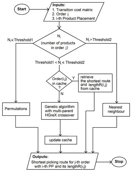
Figure 4.
Order picking route optimization.
During the order picking route optimization the locations of products are constant. The product locations are changed by Algorithm 1 only before each round of order picking route optimization. As discussed in Section 5.1, the order picking route starts from the entrance, then visits all locations of products listed in the current order and returns to the warehouse entrance. The task is to optimize the sequence of visiting the locations to obtain the shortest route.
There are two main families of approaches to finding the shortest routes connecting a list of locations—the local search methods (e.g., nearest neighbor or k-opt [28]) and population methods (e.g., genetic algorithms or ant colony optimization [28]). In the Nearest Neighbor Algorithm, we always go from the current location to the nearest yet not visited location. In this way the algorithm implements local search. The local search guaranties finding the nearest location to the current location with 100% probability. However, the drawback of the local search approaches is that they do not include the global view of the situation. Although there was some research to improve these methods, the population methods still have the advantage of applying the global search. A sample route determined with the nearest neighbor, which shows the problems of this method, is shown in Figure 5.
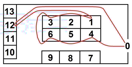
Figure 5.
A sample route (in red) connecting the locations 0, 4, 6, 2, 1, 12 determined with the Nearest Neighbor Algorithm.
As will be shown in the experimental evaluations in Section 6 and as it is also known from previous studies [29], when the Nearest Neighbor Algorithm is used instead of genetic algorithms for that kind of problems, the calculation time can be dramatically reduced, however at the cost of worse results (on average 10% longer routes).
To determine the shortest route for completing each order, our method can use three different algorithms:
- Iterating through half of the possible permutations (as the transition cost matrix is symmetric—we can start the order completion from the end or from the beginning of the determined route, so we do not need to check all permutations, but only half of them). This method is 100% accurate, but is the slowest one expect for very short orders. As its complexity is , it is impractical for orders above 10 positions and technically impossible to use for orders over 15 positions.
- Genetic algorithm with the multi-parent HGreX crossover operator. This method is faster than iterating over permutations, but does not guarantee finding the best solution, but only the solution close to the best one. (The basic version of the HGreX crossover is presented in Section 4.3 and the multi-parent extension in Section 5.4.1.) The fitness of the i-th order picking route is given by Equation (5). takes larger values for better individuals to ensure that they have higher probability of being selected as parents, while take smaller values for better individuals, as this value expresses the route length.where is a coefficient, which determined the strength of the selection (the lower , the stronger preference for the individuals representing shorter routes) is the maximal and is the minimal length of the order picking route in the population. This ensures that the re-scaled proportion between the maximal and minimal fitness is constant during the optimization (see Section 5.2 for explanations).
- Nearest Neighbor Algorithm. This is the fastest method. It also does not guarantee finding the best solution, and in application to our problem it usually finds worse solutions than genetic algorithms.
To provide the optimal trade-off between the accuracy and the speed of the route optimization, the three above algorithms can be applied and the values and are used to determine, which particular algorithm will be used for a given order, depending on the number of products in the order (see Algorithm 2 and Figure 4).
The number of possible order picking routes is equal to the number of permutations of a k-element set, which is . If there are fewer than products in a given order than it is faster to evaluate half of possible permutations (for there are various routes to examine.) than to use genetic algorithms. For we need to evaluate permutations. On the other hand genetic algorithms are usually able to find the solution evaluating fewer routes (e.g., with population of 50 individuals and 10 iteration, what gives only 500 evaluations). However, genetic algorithms have additional time overhead for operations as selection, crossover, generating random numbers, and so forth. So for 7 products in the order the calculation time is comparable and for more than seven products, genetic algorithms are faster. Thus we propose to set .
As can be seen in Section 6, the results obtained with genetic algorithms with multi-parent HGreX crossover are better those obtained with Nearest Neighbor Algorithms. On the other hand Nearest Neighbor Algorithm is faster than genetic algorithms. However, its speed advantage is much higher in a single optimization of the route, where it can be two orders of magnitude faster. In our system, when the route optimization is an iteratively performed sub-process of the product placement optimization, the differences in speed between these two methods is much lower, below one order of magnitude. There are two reasons for that. The first one is that there is implemented cashing of the already calculated routes (see details in Section 5.4.2). The caching overhead is comparable to the computational effort of Nearest Neighbor Algorithm, so it can only accelerate the genetic algorithm based route calculation. The second reason is that the time of running the main process (product placement optimization) is the same in both cases.
indicates above which number of products in the order Nearest Neighbor Algorithm should be used to optimize this order picking route. The recommendation to obtain the best results is to set to such high value that the Nearest Neighbor Algorithm will not be used at all (e.g., ). However, if our data is very big and computational and time resources are limited, we can set and and thus only the Nearest Neighbor Algorithms will be used for the route optimization. Sometimes it happens that there are only very few long orders (e.g., two orders of 50 products and all remaining orders below 20 products), so these few orders will not have significant influence on the final product placement and we can use Nearest Neighbor Algorithm for them to accelerate the calculations and genetic algorithms for all other orders (in this case by setting for example, ).
5.4. Improvements and Accelerations of the Process
We use the following improvements to obtain better results and to accelerate the process: multi-parent crossover operator, order grouping, caching product placement costs and order picking routes of evaluated individuals, multiple restart, switching among permutations/genetic algorithms/nearest neighbor for route optimization, and parallelization of the process. In the following subsections we present particular improvements. Influence of these improvements on the obtained results is evaluated experimentally and presented in tables and figures in Section 6.
5.4.1. Multi-Parent Crossover Operators
As the use of multi-parent crossover operators can significantly accelerate (up to three times) the convergence speed of the classical genetic algorithms [30,31] (as well their single-objective as multi-objective version built upon the NSGA-II algorithm [32]), one of the ideas of this work was to apply the multi-parent approach to the crossover operators in the route and product placement optimization problems in hope that it can provide better results.
There is also another rationale behind increasing the number of parents in the HGreX crossover operator. In the Nearest Neighbor Algorithm the positions are added one by one to the route; each time the closest position is appended to the last position. In the extreme case, when we have a big population so that almost each possible two-element sequence exists in the population and the number of parents in the multi-parent HGreX crossover equals the population size - the so constructed genetic algorithm becomes equivalent to the nearest neighbor search. But on the other hand increasing the number of parents only a little bit, may add the local search component to the genetic algorithms and thus improve the results.
Let us assume that we will use four parents to create each child.
- P1 = [ A B C D E F G H ]
- P2 = [ E G F H A C B D ]
- P3 = [ G H A E B F C D ]
- P4 = [ E F H D B A G C ]
Let us start from the fist position in P1, this is from A. Let us assume that there are the following distance d(A,B) = 12, d(A,C) = 15, d(A,E) = 18, d(A,G) = 11. Since in this the distance d(A,G) is the smallest the next position in the child will be G.
- Ch = [ A G _ _ _ _ _ _ ]
- and the values remaining in the parents:
- P1 = [ B C D E F H ]
- P2 = [ E F H C B D ]
- P3 = [ H E B F C D ]
- P4 = [ E F H D B C ]
Then Let us assume that there are the following distance d(G,H) = 12, d(G,F) = 8, d(G,H) = 7, Since in this the distance d(G,H) is the smallest the next position in the child will be H, and so on. Conflict resolving is implemented in the same way as in the two-parent version of the operator. In case of AEX we were appending the consecutive positions to the child sequentially from consecutive parents.
We conducted the experiments with various number of parents and the conclusion was that for this problem about 8 parents is the optimal number for the modified HGreX crossover operator. As a result of applying multiple parents for the HGreX crossover, about a two-fold reduction of the number of iterations was observed, but what is more important, also shorter order picking routes were obtained (see the experimental results in Section 6 for details). On the other hand, increasing the number of parents for the AEX crossover did not significantly change the results.
5.4.2. Caching Cost of Product Placements and Lengths of Order Picking Routes
In product placement optimization the computational effort of calculating cost (see Algorithm 1) of an given product placement and then based on it the fitness value of an individual is high, as it requires finding the shortest picking routes for all orders. Practically always either some parents are promoted to the next generation or some children are identical to some parents (even more in the final stages of the optimization). In this case, we do not calculate the cost of such an individual, but instead we directly assign the already calculated and cached cost of the previous identical individual (See Algorithm 1 and Figure 2). We also check the cache after mutation.
The situation with order picking route optimization with genetic algorithms is different. Here the computational effort of calculating the route length and determining the fitness of an individual is low and there is no use to implement caching for that. However, the cost of calculating the shortest route for an order (which may require several thousands calculations of route lengths represented by all individuals in all iteration of the optimization) is much higher and it makes a sense to implement cache here. Thus before calculating the shortest route for a given order (See Algorithm 2 and Figure 4), the cache is checked if it already contains the route for the current order j, where all the positions of products in the warehouse were the same. To clarify this, if the whole product placement can be found in cache, the sub-process of route calculations is not invoked from the main process, as the cost of this product placement is retrieved from cache. However, if the product placement differs on some positions, the sub-process is invoked and it is checked for each order, if the positions in the product placement occupied by the products contained in the current orders already exist in the cache. If so, the route length is retrieved from the cache. Otherwise it is calculated and the cache is updated. The order cache is used only for route calculation with genetic algorithms. (See Algorithm 1 and Figure 2).
The caching is not used for the Nearest Neighbor Algorithm, as the time overhead for the cache is comparable to the time used by nearest neighbor. For the same reason the cashing is not used with very short orders, where the shortest route is determined by permutations.
The caching obviously does not influence the results of the optimization and only allows to accelerate it. It is also worth noticing that the caching is more effective at the later stages of the optimization, as at the beginning the individuals change rapidly. In our experiments the caching allowed to accelerate the product placement optimization several times (see Section 6).
5.4.3. Multiple Restart
It may take many iterations for genetic algorithms to converge to the optimal solution. However, the fastest progress occurs at the beginning of the optimization. Genetic algorithms use some random numbers and thus are a stochastic process and as a result different solutions can be found with consecutive runs of the optimization. We observed that in the product placement optimization the best approach is to run the optimization several times only for a few iterations and save the current population. Then the optimization will continue only with the population of the best solution. It is a reasonable approach, because most frequently the optimization, which starts as the best also ends as the best. Thus this method allows joining time efficient optimization with good results (see the experimental verification in Section 6).
5.4.4. Order Grouping
All orders containing the same set of products are grouped together into one order. In this way the optimal picking route for this order has to be determined only once. For the purpose of calculating the cost and fitness of a given product placement, the length of the obtained route is multiplied by the number of the orders consisting of the same products (see Algorithm 1).
5.4.5. Three Route Optimization Methods
As described in Section 5.3, for the optimal balance between calculation speed and accuracy of the results, the order picking route in Algorithm 2 can be optimized with permutations (only short routes), genetic algorithms or the Nearest Neighbor Algorithm.
5.4.6. Process Parallelization
Genetic algorithms scale well for parallel implementations in the cases, where the cost of calculating the fitness function is high, because in these cases there is no need for frequent communication among threads. It is exactly the case of product placement optimization, where using any number of CPU cores up to the number of individuals in the population results in practically a linear increase of performance in the function of the number of CPU cores. Moreover, if there are more CPU cores available than the population size, it makes sense to increase the population size, at least up to three times to use more CPU cores. Although after exceeding the optimal population size the scaling with the growth of CPU number is no longer linear, this implementation is very simple. The other alternative with few hundreds of available CPU cores is to parallelize the calculation of particular order picking routes, but since we did not have access to such computational resources, we were not able to verify the efficiency of this approach.
6. Experimental Results
In this section we experimentally evaluate the method and improvements presented in the previous sections.
We conducted the experiments with our own software, created in C# language. The source code and the data used in the experiments (warehouse plans with lists of corresponding orders) are available from the web page www.kordos.com/appliedsciences2020. Three of these warehouse structures (floor plans) and some sample orders for the warehouse are additionally presented in Figure 6 and Figure 7.
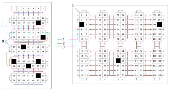
Figure 6.
Samples warehouse structures (floor plans) of the warehouses w5 and w1 used in the experiments. Each numbered cell represents one product location. Blue lines show the distance of 1 unit, red lines of 2 units and green lines of 3 units.
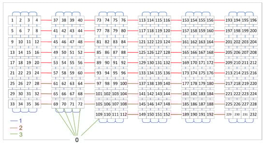
Figure 7.
A sample warehouse structure (floor plan) of the warehouse w2 used in the experiments. Each numbered cell represents one product location. Blue lines show the distance of 1 unit, red lines of 2 units and green lines of 3 units.
The following algorithms of order picking route optimization were evaluated—nearest neighbor, genetic algorithms with HGreX crossover, genetic algorithms with multi-parent HGreX crossover.
The following algorithms of product placement optimization are evaluated: genetic algorithms with AEX crossover, genetic algorithms with multi-parent AEX crossover, genetic algorithms with multi-parent AEX crossover and multiple restart.
As we could not find in literature a complete automatic solution for product placement optimization, which considers the order picking routes, as the solution presented here (see Section 1 and Section 4.2), we obviously can not compare numerically our solution to other solutions on the same data.
First we evaluated the multi-parent modifications of the HGreX crossover operator to determine the optimal number of parents (see Section 5.3 and Section 5.4.1). The results are presented in Table 2 and in Figure 8. Based on our tests the population sizes of about 80–120 allowed for the fastest convergence of the process (the lowest number of fitness value calculations). For larger populations, fitness function evaluations had to be performed more times to reach to the same results, so even if it took fewer iterations, the time to reach the results was longer [33]. However, if the populations were smaller it also required more evaluations of the fitness function and if the populations were too small, the convergence of the algorithm was impossible. Only for route optimization, when the number of products in the order was 20 or less, lower sizes of population were used and larger populations may be useful for longer chromosomes than those we used in the experimental evaluation.
Table 2.
A sample route length and number of iterations to obtain this length for a modified multi-parent HGreX crossover operator for an order of 60 products with fixed product placement (averages of 10 runs). in the last column denotes the result obtained for the Nearest Neighbor Algorithm.
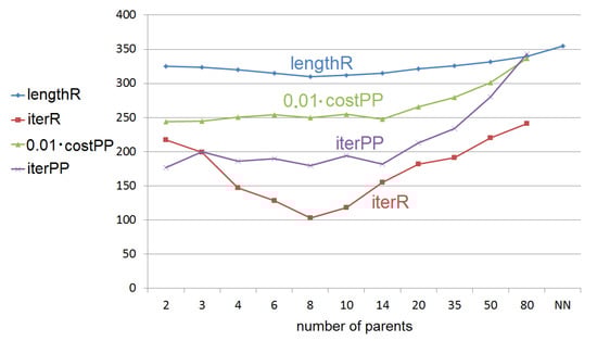
The stopping criterion for experiments shown in Table 2 was 20 iterations without improvement of the best individual. The number of reported iterations is the number after which the best individual was found. As it can be seen, increasing the number of parents in the crossover operator definitely reduces the number of required iterations (up to two times for 8 parents in this case) and what is more important, allows for obtaining better fitness values. However, when using more parents than the optimal number, the optimization again slows down and using more than 20 parents also the obtained route lengths are beginning to deteriorate (to increase). As discussed in Section 5.3, for large number of parents the HGreX operator behaves almost like the nearest neighbor search method, and also its performance tends to the same value.
The number of iterations used by the genetic algorithm with the HGreX crossover is comparable to that required by other modern crossover operators to find the shortest route for comparable population size [34]. Even if running the optimization for more iterations may find a little shorter route, there is usually no further gain for the product placement cost, as this only very rarely triggers the change of product locations. For the very rarely occurring orders it is enough to run the optimization for fewer epochs or to use Nearest Neighbor Algorithm, independently of the order length, because the quickest improvement occurs at the beginning of the optimization and the influence on the optimal product placement of very rare orders is also very low, as they are dominated by the more frequent orders.
Next we tested the usefulness of the multi-parent AEX crossover in product placement optimization. Since AEX does not use the cost of transitions between two elements, the parents for each element were chosen randomly. The results for a warehouse with 232 locations (chromosome length was 232 elements) are presented in Table 3. Based on the experiments we concluded that it is enough to use two-parent AEX crossover in product placement optimization, as increasing the number of parents did not cause any gain and if the number was 20 or more, the drop in the method effectiveness was observed.
Table 3.
The product placement cost as sum of order picking route lengths (the lower the better—see Equation 2) and number of iterations to obtain this cost for a modified multi-parent AEX crossover operator for the warehouse size of 232 locations and a list of 80 orders, using an 8-parent HGreX for route optimization (averages of 10 runs).
Multiple restart of the product placement optimization with AEX crossover (MR-AEX) proved quite useful (see Algorithm 1). In the last row of Table 4 the optimization was restarted 5 times and each time it was run for 10 iterations and then we continued only with the population of the best individual, as described in Section 5.4.3. It allowed not only to obtain lower cost, but also the standard deviation of the results was about twice lower.
Table 4.
The obtained product placement cost (the lower the better) as the sum of all order picking routes (see Equation (2)) for product placement and order picking route optimization methods with various improvements (see Section 5.4) for the six sample warehouses: w1, w2, w3, w4, w5, w6 with corresponding lists of orders, averaged over 10 optimization runs. The running times are presented in Table 5.
In the experiments presented in Table 4 we used the population size of 100 individuals for product placement optimization. For order picking route optimization we used a size of 100 individuals if the number of items was 25 or more and four times the number of items for shorter orders. The reason for choosing that population size is based on this fact, that the main cost of genetic algorithms is the evaluation of the fitness function (especially for product placement optimization). The number of the fitness function evaluations can be expressed by the multiplying population size by the number of epochs. Using larger populations, we can obtain the same results in fewer epochs. For smaller populations we also need to increase the mutation rate. However, the dependence between the population size and number of required epochs is not linear and there exists an optimal population size, which allows for the lowest number of fitness function evaluations [33]. The number also depends on the problem and on other parameters of genetic algorithms. In our experiments, the minimum was usually obtained for the population sizes between 80 and 120 individuals for the number of locations in the warehouse between 60 and 300 and then it very slowly grew, but much slower than linearly, with the increase of the warehouse. The dependence was very flat around the minimum (changing the population size e.g., from 80 to 100 individuals did not make a statistically significant difference in the number of required fitness function evaluations). However, outside of this range the dependence was more significant and for example using 1000 individuals allowed to decrease the number of epochs only about 3 times, what effectively increased the number of fitness function evaluations about 3-fold. Moreover, when the population was too small, not only the process time increased, but the process also began to be unstable and frequently was not able to converge. For this reason, a population size of 100 individuals was a safer choice than of, for example, 80 individuals.
We used the default mutation coefficients in Equation (4): , , as well in product placement as in route optimization.
Below we present some sample orders for the warehouse . The products in the orders are encoded by numbers, which are the products Ids (we cannot use letters as in the examples in previous sections, because there are not enough letters in the alphabet). The last number () of each order shows how many times such order occurs in the order list, so its completion route length can be evaluated only once and then multiplied by while calculating the final product placement cost.
- order1: 41 99 97 7 20 89 12 24 51 66 79 61 1 56 109
- order2: 71 90 9 29 84 94 19 26 64 114 100 42 81 30 108 107 101 47 6 32 96 33 28 7
- order3: 78 31 91 35 93 87 22 50 100 1 28 38 84 16 48 112 76 110 95 47 72 113 23 61 101 68 67 53 45 41 97 18 109 89 65 74 = 3
- order4: 53 61 18 36 94 24 103 38 35 12 42 89 6 30 50 14 84 114 29 15 79 95 48 52 28 25 110 22 64 109 44 11 73 33 98 97 23 75 99 87 7 51 92 93 72 17 3 = 1
Table 4 presents the detailed results for six sample warehouse structures and order lists (this is the maximum number of warehouses, which can fit in one row of the table). MP-HGreX stands for Multi-Parent HGreX with 8 parents, MR-AEX is Multiple-Restart AEX with 5 restarts, saving the population afters 10 iterations, and then continuing with the population of the best individual (see Section 5.4.3 and Figure 2 for explanations). Table 5 presents the real running times of the optimization processes (including I/O operations and Dijkstra Algorithm).
Table 5.
The real running time of the optimization processes in seconds using a computer with two Xeon X5-2696-v2 CPUs, averaged over 10 optimization runs for the experimental data presented in Table 4 and additionally for AEX/HGreX without cache (see Section 5.4.2).
The possible reduction of product placement cost depends on the character of the orders. The biggest improvement due to route optimization can be obtained for the orders containing long list of products. The highest improvement due to product placement optimization can be achieved when the orders frequently contain products of particular groups and the frequency with which particular products appear in the orders differs a lot. Thus the improvement possible to achieve is determined mostly by the properties of the orders. Thus, particular methods must be compared among each other for the same warehouse structure and for the same list of orders (This is similar, like in classification, where the possible accuracy depends on the dataset properties and various classifiers must be compared on the same data).
The cost vs. rnd. column in Table 4 contains the average relative reduction of the product placement cost calculated as cost vs. rnd. , where is the warehouse number. The last column contains statistical significance tests calculated on the whole data between two adjacent methods and therefore it is printed in-between rows of the compared methods. Since some persons prefer the T-test and others the Wilcoxon Signed Rank Test for this kind of data, we used both tests to satisfy everyone. As all the p-values in the last column of Table 4 are smaller than 0.05, it can be assumed that all the methods are significantly different from one another.
As can be seen in Figure 9 and Figure 10, the best results are obtained for the multiple restart of genetic algorithms with AEX crossover operator (MR-AEX) for product placement optimization (see Section 5.4.3 and Algorithm 1) together genetic algorithm with multi-parent HGreX crossover operator (MP-HGreX) for order picking route optimization (see Figure 4).
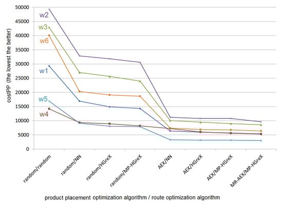
Figure 9.
Graphical representation of the data from Table 4). On horizontal axis: the optimization methods with various improvements (see Section 5.4). On vertical axis: the product placement cost (the lower the better) obtained with particular methods for the warehouses w1, w2, w3, w4, w5, w6 with corresponding lists of orders.
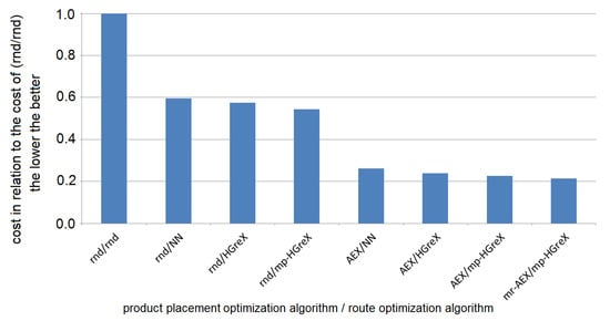
Figure 10.
Comparison of the performance of the presented methods with various improvements (see Section 5.4). On horizontal axis: the optimization method. On vertical axis: the average obtained product placement cost (the lower the better) as percentage of the cost with the random product placement and random routes over the six warehouses with order lists presented in Table 4.
7. Conclusions
Shortening the time of order picking is the most important and most beneficial factor in reducing the costs of operating the warehouse (where typically 60% are the costs are generated by order picking [1]). It can be achieved without significant investment by optimizing the locations for particular products in a warehouse and then determining the fastest order completion routes. As the search space of the solutions is enormous ( possible placements of 100 products, of 300 products) the problem cannot be analyzed by brute force methods. Thus we presented a complete, fully automatic system based on genetic algorithms, which due to applying intelligent search allows to find the optimal product placements within minutes or tens of minutes for that size of problem (depending on the computer hardware and process parameters). Even though it is not guaranteed that the optimal solution will be found with genetic algorithms, it is possible to find a very close solution to the optimal one, so that in practice it will not make a significant difference.
The presented system takes as inputs the warehouse structure (in the form of partial transition costs) and the list of orders and returns the optimal product placement and corresponding shortest order picking routes. Implementation of such a system can accelerate order picking and thus reduce the warehouse operating costs. This allows to serve more customers by the same number of employees in the same time and thus to further increase the sales and profits.
The experiments showed that using the multi-parent HGreX crossover improves the results, while for the AEX crossover adding more parents does not change its efficiency. The best results were obtained for the multiple restart genetic algorithm with AEX crossover operator (MR-AEX) for the product placement optimization process together genetic algorithm with multi-parent HGreX crossover operator (MP-HGreX) for order picking route optimization. The cost or route length caching can be used to accelerate the process. Additionally the Nearest Neighbor Algorithm can be used for route optimization to even more accelerate the process, but this is usually at the expense of a little worse result.
In the future works we are planing to implement other modifications to further improve the speed of the optimization and the quality of the obtained solutions. First we want to evaluate new crossover operators and mixtures of various operators. In the experimental comparison of Puljic [19] the mix of different crossover operators performed slightly better than HGreX. Also more advanced mixes of genetic operators were proposed [35,36]. However, we did not decide to use this approach because the implementation was definitely more complex. Instead we modified the HGreX to use multiple parents, what significantly improved the results. Łapa et al. [37] proposed the use of different operators (not only crossovers but also different mutations and other operators) for different individuals in standard genetic algorithms. We are going to adjust these approaches to the route and product placement optimizations and investigate various options.
The other branch of our future research refers to constraints in the genetic algorithm operations as in some warehouses such constraints may exist and may limit the possible locations of particular products. In the literature the typical approach to constraints in genetic algorithms is the use of penalty functions [38]. Sometimes also dominance-based methods are used [39]. However, we are going to implement it differently by embedding the mechanism directly into the crossover and mutation operators specific to that problem in order to be able to enforce the constraint effectively and to limit the computational complexity of the optimization.
Author Contributions
Conceptualization, M.K. and S.G.; Formal analysis, M.B. and S.G.; Funding acquisition, M.B. and S.G.; Investigation, M.K. and J.B.; Methodology, M.K., S.G. and J.B.; Software, M.K. and J.B.; Validation, M.B. and S.G.; Visualization, M.B. and S.G.; Writing—original draft, M.K., J.B., M.B. and S.G. All authors have read and agreed to the published version of the manuscript.
Funding
This work was supported by the Silesian University of Technology project: BK-204/2020/RM4.
Acknowledgments
The authors want to thank Michał Krzyżowski, Łukasz Mysłajek, Antoni Kopeć and Jakub Gawęda for their help in collecting and preparing the data used in this study.
Conflicts of Interest
The authors declare no conflict of interest. The founding sponsors had no role in the design of the study; in the collection, analyses, or interpretation of data; in the writing of the manuscript, and in the decision to publish the results.
References
- Bartholdi, J.J.; Hackman, S.T. Warehouse and Distribution Science. 2019. Available online: https://www.warehouse-science.com/book/index.html (accessed on 30 May 2020).
- Avdeikins, A.; Savrasovs, M. Making Warehouse Logistics Smart by Effective Placement Strategy Based on Genetic Algorithms. Transp. Telecommun. 2019, 20, 318–324. [Google Scholar] [CrossRef]
- Bolaños Zuñiga, J.; Saucedo Martínez, J.A.; Salais Fierro, T.E.; Marmolejo Saucedo, J.A. Optimization of the Storage Location Assignment and the Picker-Routing Problem by Using Mathematical Programming. Appl. Sci. 2020, 10, 534. [Google Scholar] [CrossRef]
- Van Gils, T.; Ramaekers, K.; Caris, A.; De Koster, R. Designing efficient order picking systems by combining planning problems: State-of-the-art classification and review. Eur. J. Oper. Res. 2018, 267, 1–15. [Google Scholar] [CrossRef]
- Wang, W.; Gao, J.; Gao, T.; Zhao, H. Optimization of Automated Warehouse Location Based on Genetic Algorithm. In Proceedings of the 2nd International Conference on Control, Automation and Artificial Intelligence (CAAI 2017), Sanya, China, 25–26 June 2017; pp. 309–313. [Google Scholar]
- Grosse, E.H.; Glock, C.H.; Neumann, P.W. Human factors in order picking: A content analysis of the literature. Int. J. Prod. Res. 2016, 55, 1260–1276. [Google Scholar] [CrossRef]
- Dijkstra, A.; Roodbergen, K. Exact route-length formulas and a storage location assignment heuristic for picker-to-parts warehouses. Transp. Res. Part E 2017, 102, 38–59. [Google Scholar] [CrossRef]
- Rakesh, V.; Kadil, G. Layout Optimization of a Three Dimensional Order Picking Warehouse. IFAC-PapersOnLine 2017, 48, 1155–1160. [Google Scholar] [CrossRef]
- Davarzani, H.; Norrman, A. Toward a relevant agenda for warehousing research: Literature review and practitioners’. Logist. Res. 2015, 8, 1–18. [Google Scholar] [CrossRef]
- Zunic, E.; Besirevic, A.; Skrobo, R.; Hasic, H.; Hodzic, K.; Djedovic, A. Design of Optimization System for Warehouse Order Picking in Real Environment. In Proceedings of the XXVI International Conference on Information, Communication and Automation Technologies, Sarajevo, Bosnia and Herzegovina, 26–28 October 2017; Volume 26. [Google Scholar]
- Dharmapriya, U.; Kulatunga, A. New Strategy for Warehouse Optimization—Lean warehousing. In Proceedings of the 2011 International Conference on Industrial Engineering and Operations, Kuala Lumpur, Malaysia, 22–24 January 2011. [Google Scholar]
- Affenzeller, M.; Wagner, S.; Winkler, S.; Beham, A. Genetic Algorithms and Genetic Programming: Modern Concepts and Practical Applications; CRC Press: Boca Raton, FL, USA, 2018. [Google Scholar]
- Simon, D. Evolutionary Optimization Algorithms; Wiley: New York, NY, USA, 2013. [Google Scholar]
- Ławrynowicz, A. Genetic Algorithms for Advanced Planning and Scheduling in Supply Networks; Difin: Warsaw, Poland, 2013. [Google Scholar]
- Xu, W.; Jia, H. Research on Storage Location Optimization Based on Genetic Algorithms. J. Phys. Conf. Series 2019, 1213, 032020. [Google Scholar] [CrossRef]
- Hassanat, A.B.A.; Alkafaween, E. On Enhancing Genetic Algorithms Using New Crossovers. Int. J. Comput. Appl. Technol. 2017, 55. [Google Scholar] [CrossRef]
- Hwang, H. An improvement model for vehicle routing problem with time constraint based on genetic algorithm. Comput. Ind. Eng. 2002, 42, 361–369. [Google Scholar] [CrossRef]
- Tan, H.; Lee, L.H.; Zhu, Q.; Ou, K. Heuristic methods for vehicle routing problem with time windows. Artif. Intell. Eng. 2001, 16, 281–295. [Google Scholar] [CrossRef]
- Puljić, K.; Manger, R. Comparison of eight evolutionary crossover operators for the vehicle routing problem. Math. Commun. 2013, 18, 359–375. [Google Scholar]
- Davarzani, H.; Norrman, A. A note on two problems in connexion with graphs. Numer. Math. 1959, 1, 269–271. [Google Scholar]
- Floyd, R.W. Algorithm 97: Shortest Path. Commun. ACM 1962, 5. [Google Scholar] [CrossRef]
- Bellman, R. On a routing problem. Q. Appl. Math. 1958, 16, 87–90. [Google Scholar] [CrossRef]
- Hart, P.E.; Nilsson, N.J.; Raphael, B. A Formal Basis for the Heuristic Determination of Minimum Cost Paths. IEEE Trans. Syst. Sci. Cybern. 1968, 4, 100–107. [Google Scholar] [CrossRef]
- Kreinovich, V.; Olac, L.F.; Quintana, C. Genetic Algorithms: What Fitness Scaling Is Optimal? Cybern. Syst. 2001, 24. [Google Scholar] [CrossRef]
- Razali, N.M.; Geraghty, J. Genetic Algorithm Performance with Different Selection Strategies in Solving TSP. In Proceedings of the World Congress on Engineering WCE 2011, London, UK, 6–8 July 2011. [Google Scholar]
- Hassanat, A.E.A. Choosing Mutation and Crossover Ratios for Genetic Algorithms—A Review with a New Dynamic Approach. Information 2019, 10, 390. [Google Scholar] [CrossRef]
- Otman, A.; Tajani, C.; Abouchabaka, J. Analyzing the Performance of Mutation Operators to Solve the Travelling Salesman Problem. arXiv 2012, arXiv:1203.3099. [Google Scholar]
- Nilsson, C. Heuristics for the Traveling Salesman Problem; Technical Report; Linkoping University: Linkoping, Sweden, 2003. [Google Scholar]
- Kaabi, J.; Harrath, Y. Permutation rules and genetic algorithm to solve the traveling salesman problem. Arab. J. Basic Appl. Sci. 2019, 26, 283–291. [Google Scholar] [CrossRef]
- Kordos, M.; Łapa, K. Multi-Objective Evolutionary Instance Selection for Regression Tasks. Entropy 2018, 20, 746. [Google Scholar] [CrossRef]
- Kordos, M.; Arnaiz-González, A.; García-Osorio, C. Multi-Objective Evolutionary Instance Selection for Regression Tasks. Neurocomputing 2019, 358, 309–320. [Google Scholar] [CrossRef]
- Deb, K.; Pratap, A.; Agarwal, S.; Meyarivan, T. A fast and elitist multiobjective genetic algorithm: NSGA-II. IEEE Trans. Evol. Comput. 2002, 6, 182–197. [Google Scholar] [CrossRef]
- Kordos, M. Optimization of Evolutionary Instance Selection. Lect. Notes Artif. Intell. 2017, 10245, 359–369. [Google Scholar]
- Xin, J.; Zhong, J.; Yang, F.; Cui, Y.; Sheng, J. An Improved Genetic Algorithm for Path-Planning of Unmanned Surface Vehicle. Sensors 2019, 19, 2640. [Google Scholar] [CrossRef]
- Contreras-Bolton, C.; Parada, V. Automatic Combination of Operators in a Genetic Algorithm to Solve the Traveling Salesman Problem. PLoS ONE 2015, 26. [Google Scholar] [CrossRef]
- Contreras-Bolton, C.E. Algorithms for Variants of Routing Problems. Ph.D. Thesis, Università di Bologna, Bologna, Italy, 2019. [Google Scholar]
- Łapa, K.; Cpałka, K.; Laskowski, Ł.; Cader, A.; Zeng, Z. Evolutionary Algorithm with a Configurable Search Mechanism. J. Artif. Intell. Soft Comput. Res. 2020, 10, 151–157. [Google Scholar] [CrossRef]
- Chehouri, A.; Younes, R.; Perron, J.; Ilinca, A. A Constraint-Handling Technique for Genetic Algorithms using a Violation Factor. J. Comput. Sci. 2016. [Google Scholar] [CrossRef]
- Ponsich, A.; Azzaro-Pantel, C.; Domenech, C.; Pibouleau, L. Constraint handling strategies in Genetic Algorithms application to optimal batch plant design. Chem. Eng. Process. Process. Intensif. 2008, 47, 420–434. [Google Scholar] [CrossRef]


© 2020 by the authors. Licensee MDPI, Basel, Switzerland. This article is an open access article distributed under the terms and conditions of the Creative Commons Attribution (CC BY) license (http://creativecommons.org/licenses/by/4.0/).