Article

Correlation of Concurrent Extreme Metocean Hazards Considering Seasonality

by
Felícitas Calderón-Vega
1,2,
Adrián-David García-Soto
1,* and
César Mösso
2,3
1
Department of Civil Engineering, Universidad de Guanajuato, Juárez 77, Zona Centro, Guanajuato P.C. 36000, Mexico
2
Laboratori d’Enginyeria Marítima, Universitat Politècnica de Catalunya, Jordi Girona 1-3, Mòdul D1, Campus Nord, 08034 Barcelona, Spain
3
Centre Internacional d’Investigació dels Recursos Costaners, Jordi Girona 1-3, Mòdul D1, Campus Nord, 08034 Barcelona, Spain
*
Author to whom correspondence should be addressed.
Appl. Sci. 2020, 10(14), 4794; https://doi.org/10.3390/app10144794
Submission received: 17 June 2020 / Revised: 8 July 2020 / Accepted: 9 July 2020 / Published: 13 July 2020
(This article belongs to the Special Issue Advances in Multihazard Science)

Abstract

:
Simultaneous occurrence of metocean variables can present a multihazard to maritime systems. However, simplified design approaches to assess simultaneous significant wave heights and wind velocities are lacking, especially if seasonality is considered. This is addressed in this study by using extreme significant wave heights and companion wind velocities recorded in the Gulf of Mexico. Time-dependent, generalized extreme value (GEV) models and classical regression are the basis to propose a simplified approach to estimate correlated extreme significant wave heights and wind velocities associated with given return periods, accounting for seasonality and including measures of uncertainty. It is found that the proposed approach is a new but simple method to adequately characterize the concurrent extreme metocean variables and their uncertainty. It is concluded that the method is an effective probabilistic design tool to determine simultaneous extreme significant wave heights and companion wind velocities for desired return periods and seasonality.

1. Introduction

Maritime structures, such as offshore facilities, breakwaters and other systems, are subjected to the effect of metocean variables, including extreme waves and extreme winds. These metocean variables can be considered as hazards that impose demands to these systems. Metocean variables can be characterized with a probability density function (PDF) frequently adopted from extreme value theory [1]. Among the metocean variables, extreme waves and winds can impact offshore facilities [2]; correlation of these two variables is important for design because they can occur simultaneously [3].
Recent studies on extreme waves and winds include the assessment of significant wave heights in the South China Sea using hindcast data [4], wind models to simulate waves in the South China Sea and the East China Sea [5], the use of radar images to estimate significant wave height [6], wave height forecasting during extreme events [7], assessment of wave heights by using generalized Pareto and Gumbel distributions [8], uncertainty assessment in extreme significant wave height by using different techniques [9] and a review on available wind–wave models and their limitations [10]. Additionally, hindcast for wind–wave for several decades was calculated and compared with observed data for estimating wave climate change and for risk analysis [11,12]. Regarding studies on generalized extreme value (GEV) distribution, they are used lately to model different variables. For instance, GEV distributions resulted in a very adequate model of precipitation and evapotranspiration in India [13], and are also implemented in software to model annual maximum precipitation [14]; some variants of the method that consider nonstationarity are also found in the literature applied to river water levels [15]. The use of GEV for modeling extreme typhoon heading directions [16], joint PDFs for wave height and period [17] and for modeling extreme wave heights in the Mediterranean and at Portuguese locations [18,19] are also reported in recent literature. This shows that GEV models are a tool used currently to effectively characterize metocean and other variables. Nevertheless, no single study in recent literature on GEV reports a proposal like the one contained in the present study.
Studies regarding correlation of metocean variables are also available in the literature. Contour maps and joint distribution of environmental variables are used for marine and coastal design. Current approaches are summarized in [20], where nonparametric methods, copula models, hierarchical conditional models and conditional extremes models are used to compute contour maps for joint occurrence of significant wave height and wave period. Some of the important highlights reported in [20] include: that joint probabilities are important for reliability analysis as stipulated in guidelines and standards, that simultaneous occurrence of extreme events at prescribed return periods is of interest, that the values associated with such return periods are not uniquely defined (except by independent or perfectly correlated cases), that the problem may need to be studied in a case-by-case basis, that different techniques may be more suitable than others depending on the problem to be addressed, among other issues.
Studies on correlated metocean variables accounting for seasonality are also found in the literature. For instance, Vanem [21] develops weekly contour maps for wave height and wave period using selected return periods. The season-specific variability of simultaneous metocean variables can be important for planning [21]. In [21], a proposal is based on normalizing the data using the mean and standard deviation to remove seasonality, which can be added back later; it is argued that the whole set of data (i.e., from all the seasons) can be taken advantage of, opposite to fitting the data into separate bins, which results in a decrease in the fitted data. Nevertheless, the use of separate bins to fit the data is also used as an alternative to account for seasonality of metocean variables [22,23,24,25].
In the literature review, the use of hindcast data, consideration of seasonality and the use of different PDFs are found. However, most studies are based on complex or time-consuming methodologies. Nonetheless, Bitner-Gregersen [26] reports a summary of simplified expressions of practical applicability contained in guidelines, which will be useful later in this study. The study of concurrent metocean variables at different locations is important, since specific features of metocean climate depend not only on the region but also on the specific location [26]. Simple techniques to assess simultaneous significant wave heights and companion wind velocities are lacking, especially to account for seasonality.
The main objective of this study is to develop a simple approach to correlate extreme significant wave height and companion wind velocity for given return periods and accounting for seasonality. Time-dependent GEV models and classical regression applied to data from a buoy located in the Gulf of Mexico are used as the basis of this study. The results can be useful for design projects on multihazards of maritime systems, since extreme waves and companion winds can translate into simultaneous demands imposed on these systems.

2. Significant Wave Height and Wind Velocity Data Used

The significant wave heights and wind velocities are obtained from a buoy in the Gulf of Mexico operated by the National Data Buoy Center (NDBC, www.ndbc.noaa.gov). It is in the Gulf of Mexico at 25.942° N 89.657° W, denoted as buoy 42,001 [27]; its data were used in a previous study [28]. It is selected to illustrate the proposed approach because of its location at open sea and because it has recorded simultaneous information of metocean variables since 1975, but the method can be readily extended to other buoys at open sea in the Gulf of Mexico or anywhere else. For the scope of the present study, the maximum monthly significant wave heights, Hs, recorded at buoy 42,001 are used, together with the wind velocity, Vw, recorded and listed in [27] within the same time bin. It is pointed out that Vw is not necessarily the monthly maximum wind speed, but the one which occurred simultaneously with the monthly maximum significant wave height (level of resolution within [27]); thus it is also referred to as companion wind. The significant wave height and wind speeds used are those defined in [27], denoted as WVHT and WSPD [27], respectively. The wind velocity is averaged over an eight-minute period and is recorded at 3.6 m above sea level [27]. For the scope of this study, the data are used as directly given in [27]. Both metocean variables, Hs and Vw, are to be probabilistically characterized with a model that can represent seasonality effects, as described in the following sections.

3. Extreme Value Analysis Considering Seasonality

In this section the method to perform the extreme value analysis considering seasonality is briefly summarized, since details are described in a previous study [28]. In the next section, the model is to be first applied separately to the significant wave height and wind velocities.
The model employs the generalized extreme value (GEV) family of distributions [29]. Instead of characterizing a random variable with the Gumbel, Weibull or Frechet PDF or cumulative functions (CDF), a single mathematical expression can be used, since it can represent the three. This is the GEV model used here and given by:
G ( x ) = exp { [ 1 + ξ ( x μ ψ ) ] + 1 ξ } ξ 0 G ( x ) = exp { exp [ ( x μ ψ ) ] } ξ = 0
or given by:
g ( x ) = 1 ψ [ 1 + ξ ( x μ ψ ) ] + ( 1 + 1 ξ ) exp { [ 1 + ξ ( x μ ψ ) ] + 1 ξ } s i ξ 0 g ( x ) = 1 ψ exp ( x μ ψ ) exp [ exp ( x μ ψ ) ] s i ξ = 0
if the PDF is to be used. In Equations (1) and (2), [a]+ implies the max (a,0), −∞ < μ < ∞ is the location parameter, ψ > 0 is the scale parameter and ξ the shape parameter; ξ leads to the Gumbel distribution when equal to zero, and to the Frechet and Weibull distributions when ξ > 0 and ξ < 0, respectively.
For the GEV models of Hs and Vw, the block maxima concept is used. The monthly maximum Hs values are considered as the samples for the extreme value analysis, while for the samples of Vw, they do not necessarily correspond to the maximum, but to the companion wind velocities recorded when Hs occurred. The seasonality is a cyclic behavior linked to climatic patterns, which behave in a sinusoidal way every year. The common stationary model for extreme value analysis is extended to include time dependency. It is assumed that monthly maxima and companion values are independent random variables. Furthermore, it is assumed that the maximum (or companion) monthly values Zt of observed Hs and Vw in month t follows the GEV distribution referred to above, which location μ(t) > 0, scale ψ(t) > 0 and shape ξ (t) parameters are a function of time.
The CDF of Zi is given by:
F t ( z ) = { { exp { [ 1 + ξ ( t ) ( z μ ( t ) ψ ( t ) ) ] + 1 ξ ( t ) } exp { exp [ ( z μ ( t ) ψ ( t ) ) ] }
where [a]+ = max [a,0].
The GEV parameters account for nonstationarity with the following expression:
θ = { μ ( t ) = β 0 + β 1 cos ( 2 π t ) + β 2 s i n ( 2 π t ) + β 3 cos ( 4 π t ) + β 4 s i n ( 4 π t ) ψ ( t ) = α 0 + α 1 cos ( 2 π t ) + α 2 s i n ( 2 π t ) + α 3 cos ( 4 π t ) + α 4 s i n ( 4 π t ) ξ ( t ) = γ 0 + γ 1 cos ( 2 π t ) + γ 2 s i n ( 2 π t ) + γ 3 cos ( 4 π t ) + γ 4 s i n ( 4 π t )
where mean values are denoted with β 0 , α 0 and γ 0 , harmonic amplitudes by β i , α i and γ i (for i = 1, 2) and subharmonic amplitudes by β i , α i and γ i (for i = 3, 4); t is given in years. The maximum likelihood estimators for the location μ, scale ψ and shape ξ parameters vary during the year; the regression coefficients and the probability distribution parameters are determined through the method of maximum likelihood (MML), in which the likelihood function for the GEV model is given by:
l ( θ | t i x i ) = i = 1 m { log ψ ( t i + ( 1 + 1 ξ ( t i ) ) log [ 1 + ξ ( t i ) ( x i μ ( t i ) ψ ( t i ) ) ] + + [ 1 + ξ ( t i ) ( x i μ ( t i ) ψ ( t i ) ) ] + 1 ξ ( t i ) }
As previously noted, the location μ ( t ) > 0, scale ψ(t) > 0 and shape ξ (t) parameters are expressed in terms of harmonic functions, whose amplitudes are regression parameters to be mathematically estimated.
The selective search methodology known as stepwise approach is used to find the best model, which encompasses the forward selection and backward elimination methods, which are described elsewhere [30]. The uncertainty of the selected model is accounted for by standard errors and confidence intervals [30]. The present study proposes an approach to compute concurrent metocean variables (Hs and Vw) associated with given return periods, for which the individual values associated with each variable are required. The values associated with return periods for each variable considered separately can be obtained with the following equation:
X q ( t , θ ) = X q ( μ ( t ) , ψ ( t ) , ξ ( t ) ) = { μ ( t ) ψ ( t ) ξ ( t ) { 1 [ log ( 1 q ) ] ξ ( t ) } i f ξ ( t ) 0 μ ( t ) ψ ( t ) log [ log ( 1 q ) ] i f ξ ( t ) = 0
where q corresponds to the exceedance probability as defined by G t(x) = 1 − q and the estimated quantile, and Xq(t,θ) corresponds to the time-dependent value associated with the return period T-yr = 1/q for a metocean variable of interest.
The model described in this section is applied to Hs and Vw in the following sections; first, for each individual variable, and then subsequently, the approach to correlate both metocean variables is presented.

4. Correlating Extreme Metocean Variables

4.1. Nonstationary Models Considered Separately

The time-dependent GEV model described in the previous section is first applied separately to each of the metocean variables. The significant wave height Hs and wind velocity Vw described before are employed. Recall that while for the GEV analysis of Hs the monthly maxima from buoy 42,001 are used, the Vw data do not necessarily correspond to the monthly maximum recorded values, but to the companion wind velocities that occurred simultaneously with the monthly maximum Hs.
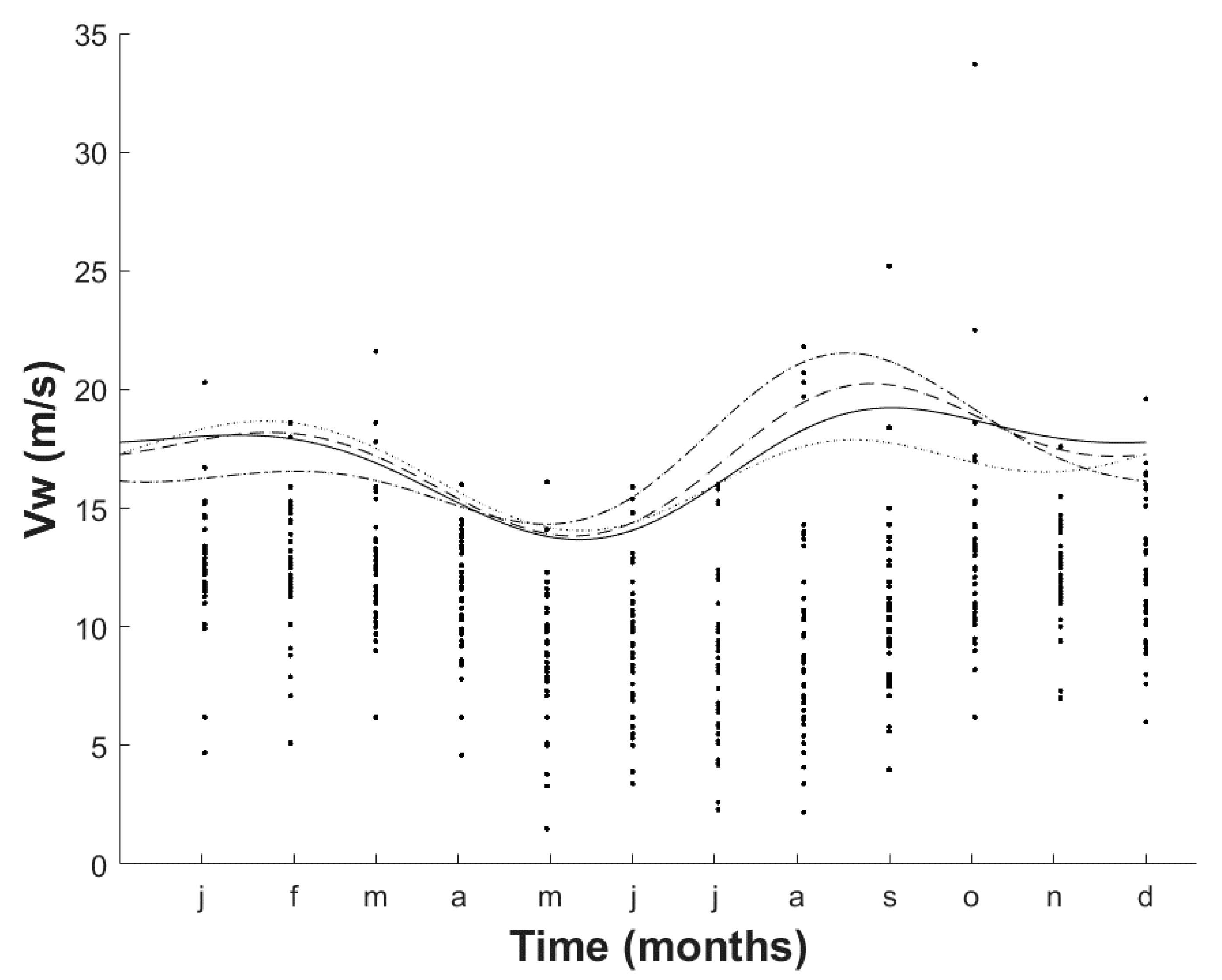
Figure 1 shows the maximum Hs recorded monthly (depicted with dots) and the 30 yr return period values, T-30, estimated with the GEV model (depicted with a solid line). As in a previous study [28], clear peaks approximately around the seasons of December–February and August–October, associated with cold fronts and hurricanes, respectively, are observed in Figure 1.
To inspect whether a difference using the updated information in the present study (i.e., with data up to 2019) and that from the previous study [28] (with data up to 2012) exists, the T-30 values reported in [28] are also depicted in Figure 1 (dashed lines). It can be observed that inclusion of recent data points in the analysis does have an effect in the projected values, leading to a decrease in the peak Hs values for hurricane and cold front seasons—more noticeable for the former—and an increase at midyear months.
To further investigate the impact of selecting different time windows in the assessment of projected values associated with a given return period, two more lines are shown in Figure 1, which were computed using the oldest (dotted line) and the newest (dashed–dotted line) maximum 20 available recorded monthly data per year; selection of at least a 20 years range for the analysis is recommended to properly characterize metocean variables probabilistically [3]. There is a noticeable impact of using these different time windows to assess the Hs values for T-30.
Determining if this could be attributed to climate change is feasible, since studies in the literature [31] report that higher or lower metocean variables could be attributed to climate change, which depends on region and location, although it is important to acknowledge uncertainty in claiming any categorical trend [31]. This potential variation in wave climate could importantly impact maritime structures [31]. Future studies are desirable to further investigate this topic; nevertheless, it can be concluded that selection of different time ranges does have an impact in the projected return values of Hs (and other metocean variables). Moreover, it is accepted that using more metocean data leads to more reliable extreme value analyses [2,3], but the use of less data and more recent data could lead to a higher projected return period value for some months. Consequently, future research and discussion on this issue is recommended.
Figure 2 is analog to Figure 1, except that Vw values are shown. Less accentuated peaks can be observed for hurricane and cold front seasons in Figure 2, perhaps because not the maximum, but the companion values are employed, even though the trends are similar, at least for the updated (solid line) and previously used [28] time ranges (dashed lines).
For the scope of this study, only models corresponding to the solid lines in Figure 1 and Figure 2 are used (i.e., the whole set of available data at buoy 42,001 is considered), although projected metocean variables for other return periods are also used. The values for other return periods, used later in this study, for each month are listed in Appendix A in Table A1 and Table A2 for Hs and Vw, respectively. No details in this study are given about the parameters of the GEV models as were provided in previous studies (e.g., [28]), since attention is focused on proposing a simplified approach to correlate extreme Hs data and their companion Vw data associated with given T-yr values. This is developed in the following section.

4.2. Simplified Approach for Return Period Correlated Values

The proposal to estimate the simultaneous occurrence of extreme metocean variables is based on a modified version of the classical linear regression technique. This consists in including estimated values from the time-dependent GEV models in the previous section—together with the simultaneously observed monthly data for maximum Hs and companion Vw—in the regression analysis, to assess how adequate is the use of the return period value of the explanatory variable (in the regression analysis sense) to predict the return period value of the other variable and its uncertainty. This is to be carried out for each month of the year to estimate seasonal extreme (and companion) values associated with given return periods, so that they can be considered as a demand which is applied simultaneously to a maritime system (or other system). From this standpoint, significant wave heights and wind velocities can be considered as concurrent extreme metocean hazards accounting for seasonality, since they can be translated into load effects affecting a given maritime structure at the same time, at any desired season of the year. Moreover, such demands are usually related to given return periods for design purposes; consequently, it is convenient to establish them in terms of return periods. This is also the case for using contour maps in ocean engineering [20].
Before proceeding to introduce the proposal, the classical regression analysis using Hs as the explanatory variable and Vw as the variable to be predicted is described as follows by using the observed data only. Buoy 42,001 is used to illustrate the procedure, but this can be extended to any buoy with simultaneous recorded metocean data. Hs is selected as the explanatory variable because it was used in a previous study [28] to investigate maxima. As noted before, Vw is not necessarily the maximum, but the wind velocity observed simultaneously with the monthly maximum Hs. Naturally, it could be considered otherwise, e.g., maximum Vw and associated simultaneously recorded companion Hs, but also other pairs of concurrent values of Hs and Vw could be selected. This aspect is discussed later. From a designer perspective, it can be thought of as selecting an Hs value and using it to predict a Vw value that is expected to occur simultaneously; then, both can be used to estimate the imposed (adding) effects of both metocean variables acting over a system, which capacity is to be designed to withstand such demand. Since both metocean variables are random, this can be expressed in mathematical terms [32,33] as:
E [ V w | H s = h s ] = b + α   h s
where the expected value of Vw, given that Hs = hs, is a linear function of hs; b and α are constants to be determined by linear regression analysis. However, guideline expressions that relate wind velocities and wave heights, as well as fitted functions found in the literature [26], commonly have the following mathematical form:
V w = b H s α
which can be linearized by taking the natural logarithm, leading to:
ln V w = β + α ln H s
where β = ln b; the notation in terms of the expected value is skipped for simplicity. Equations (7) and (9) are used in the linear regression analysis. For using Equation (9), the wind velocities and significant wave heights are first transformed into logarithmic space [33].
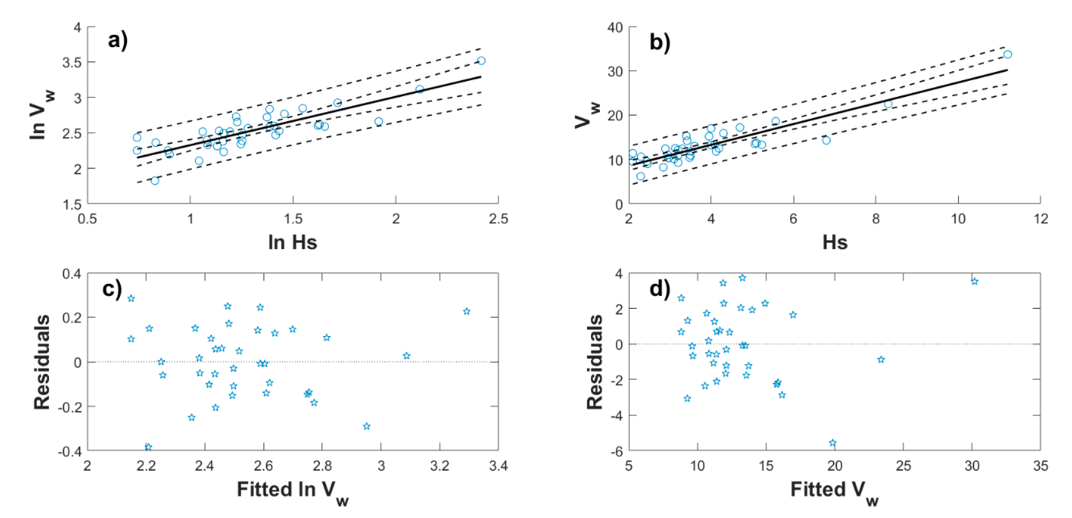
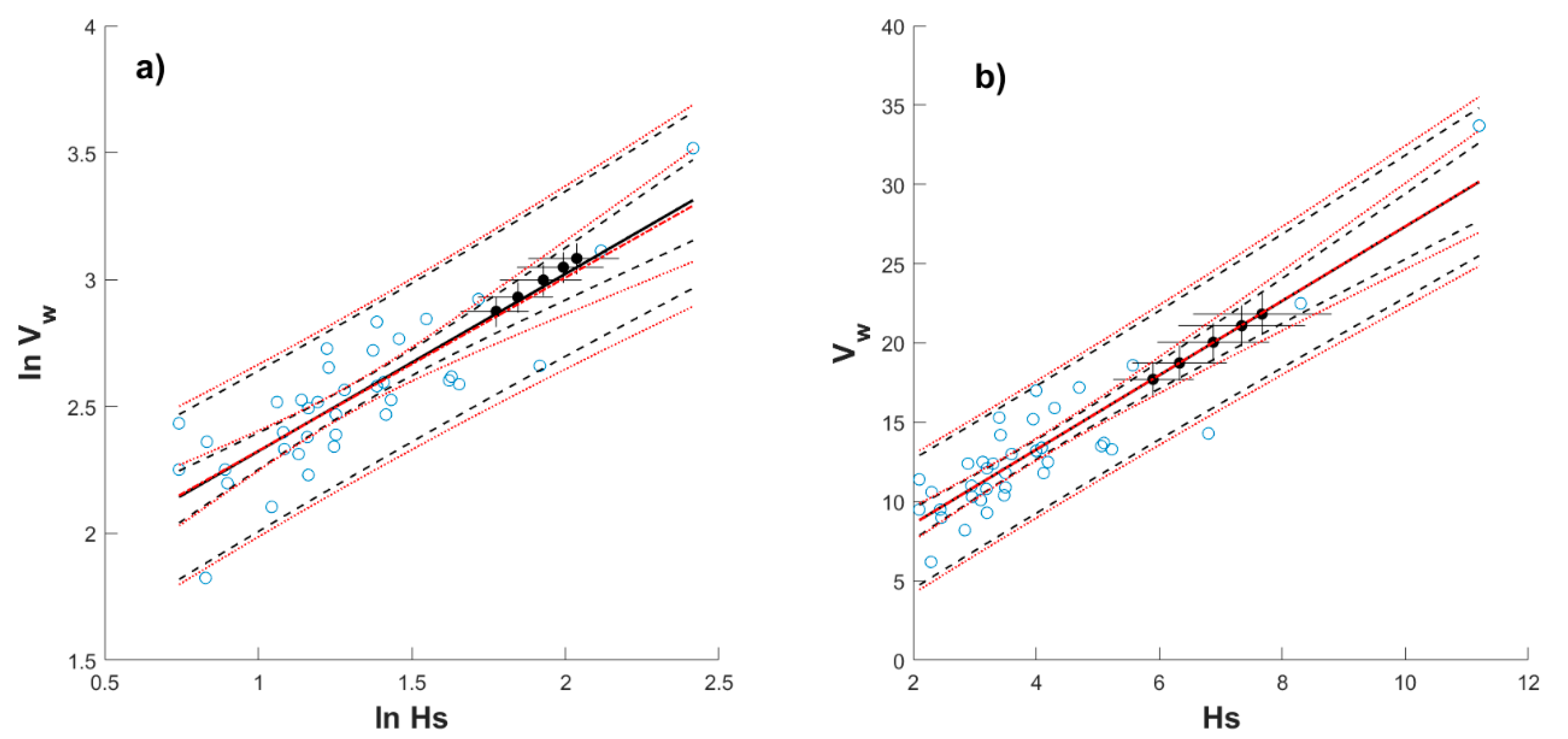
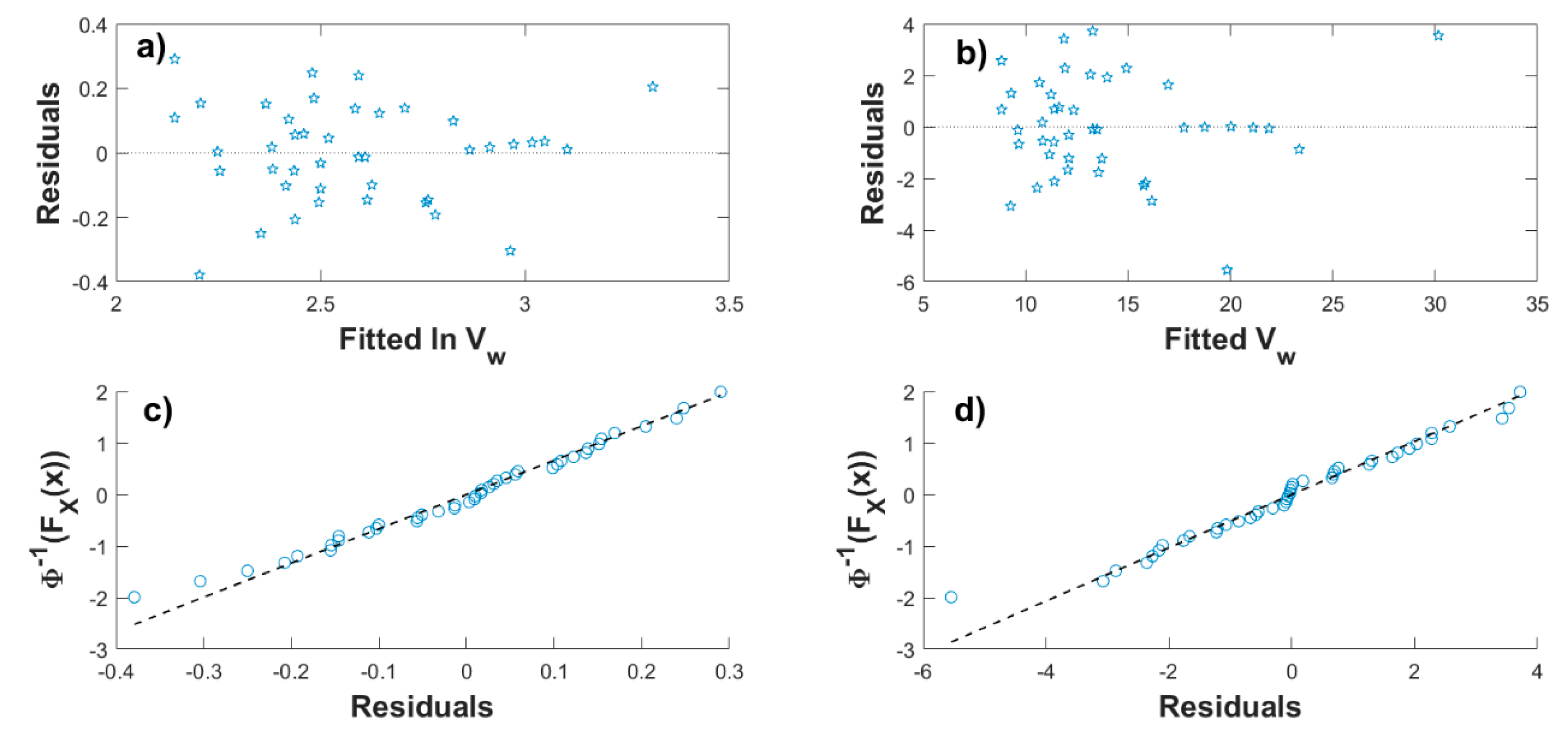
Figure 3a,b shows the linear regression analysis by using the nonlinear model (i.e., Equation (9)) and the linear model (i.e., Equation (7)), respectively, for October (around hurricane season); the residuals versus the fitted values of ln Vw (Figure 3c) and Vw (Figure 3d) are also shown.
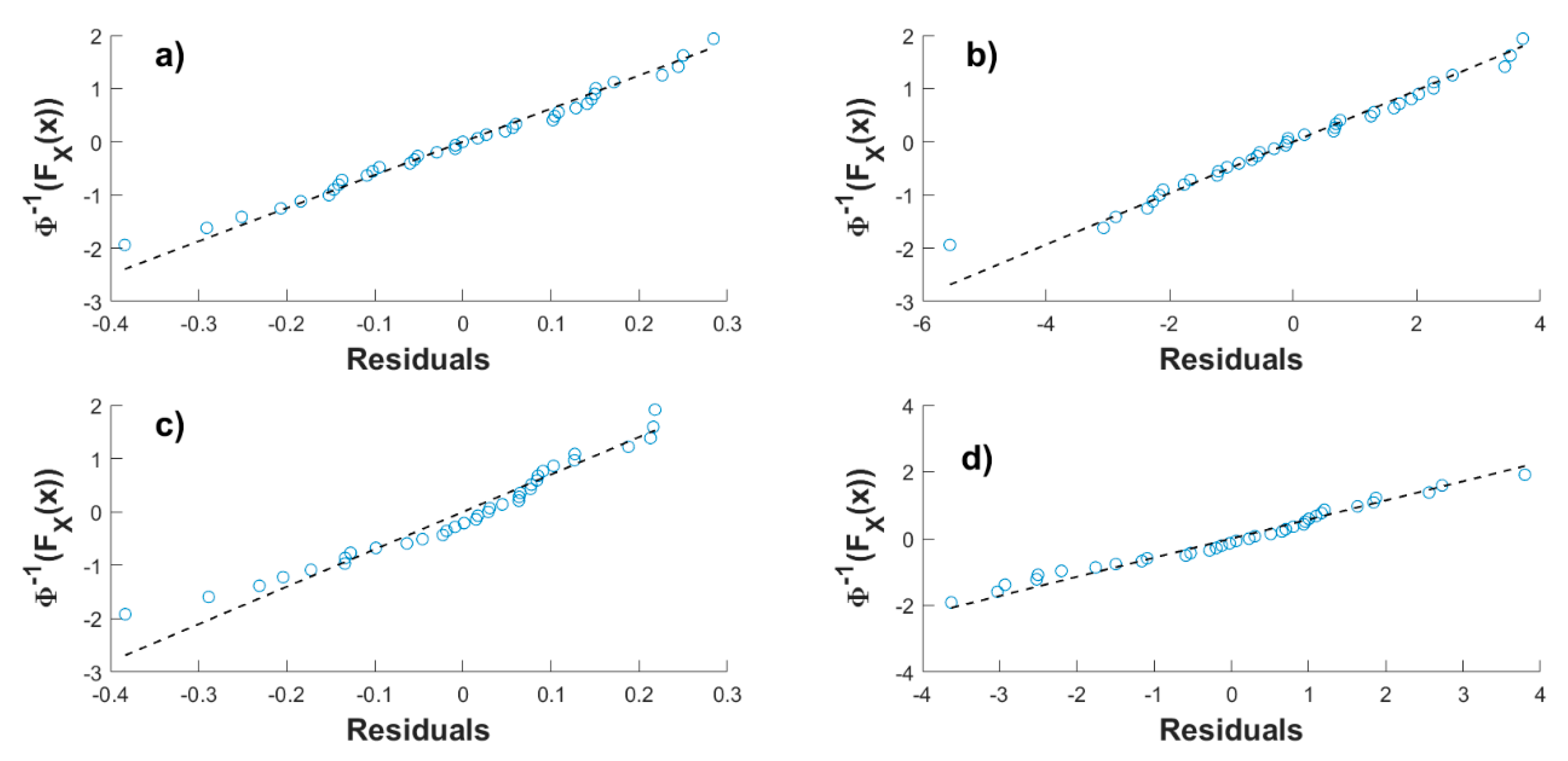
As mentioned before, the regression is first performed by using only the historical observed data, shown by circles in Figure 3a,b. It can be observed that the regression line (solid line) in both cases (i.e., Equations (9) and (7)) predicts increasing Vw for increasing Hs. This is consistent with what is reported in the literature. The 95% confidence intervals, which are measures of uncertainty for mean and future values of Vw [33,34], are also shown in Figure 3a,b (inner and outer dashed lines for mean and future values, respectively). Analysis of residuals versus predicted values indicates that the nonlinear model leads to a better scattering of the data along the horizontal axis (i.e., the model is uncorrelated) and better symmetry in the vertical axis (i.e., the zero mean assumption), indicating that the nonlinear model is better for the values observed in October. Both models roughly exhibit a normal distribution behavior in the residuals, as can be observed in Figure 4a for the model in logarithmic space and 4b for the linear model, where the normal probability papers are plotted using the cumulative probability given by i/(n + 1), where n is the number of samples (i.e., the number of residuals) and i corresponds to the number of a datapoint (a residual) in ascending order.
Figure 5 is analogous to Figure 3, except that February instead of October is considered (i.e., around cold front season). Opposite to what occurs in the regression analysis for October, the analysis for February is better represented using the linear model (Figure 5b), rather than by using the linearized model in the natural logarithmic space (Figure 5a); this can be inspected in the residuals and normal probability papers in Figure 5c,d and Figure 4c,d, for Equations (9) and (7), respectively. It is found in this study that correlation of significant weight height and wind velocity can be better represented (in terms of classic linear regression) by linear (Equation (7)) or power (Equation (9)) expressions, depending on the month of the year (e.g., hurricane season, cold front season or others). This is not clearly stated in other studies.
Nevertheless, it can be observed that both the linear or the nonlinear regression analysis lead to a fairly normal behavior of the residuals, and to a relatively uniform distribution of the variance around the mean, which could be associated with a homoscedastic behavior [33], although this varies depending on the month and type of regression considered (i.e., on using Equation (7) or Equation (9)). The error variance, σe2 is an indication of the uncertainty in the regression, and its squared root is known as the root mean squared error (RMSE). Overall, the residual analyses for all months indicate that the usual assumptions in the regression approach are met [34], and that Equation (7) and Equation (9) can be suitable alternatives. Although Equation (8) is frequently encountered in codified design and the literature [26] as indicated above, functional forms like those of Equation (7) are also found, as in the standard of the North Atlantic Treaty Organization, Standardized Wave and Wind Environments and Shipboard Reporting of Sea Conditions (NATO-STANAG 4194, see [26]), which can be expressed as:
V w = b + α H s
where the nomenclature used in the present study applies (for the NATO-STANAG 4194, b = 0 and α = 3.2). Equations with the functional form of Equations (8) and (10) are used for open sea and coastal waters; those employed for coastal waters are also linked to the fetch as an important variable [26]. In the present study, the fetch is not considered since the buoy used is located in open sea.
As shown in Figure 3 and Figure 5, the data are approximately contained within the confidence intervals for future values in all cases. It is noticed that the confidence intervals for future values can be simplified by using Equation (11a,b), for the lower and upper interval, respectively.
V w l o w = b + α H s δ σ e
V w u p p = b + α H s + δ σ e
where σe = σ e 2 is the so-called RMSE which—advantageously—is part of the information that can be obtained when a regression analysis is performed; δ is a constant value to be discussed. If Equation (8) is to be considered to derive simplified expressions for the confidence intervals, expressions like Equation (11) can be written by including ±δ times the RMSE in Equation (9), except that the RMSE corresponds to the regression in logarithmic space. If the equation in the original space is to be used to compute the expected value (i.e., Equation (8)), it can be shown with some algebraic manipulations that the 95% confidence intervals for future values can be approximated by using Equation (12a,b):
V w l o w = b H s α ( 1 e δ σ e )
V w u p p = b H s α ( e δ σ e )
The value of δ is adequate to represent the 95% confidence intervals (denoted simply as confidence intervals from now on) for future values by adopting constant values approximately between 1.9 and 2.3, depending on the season considered and for both sets of equations (i.e., Equations (11) or (12)).
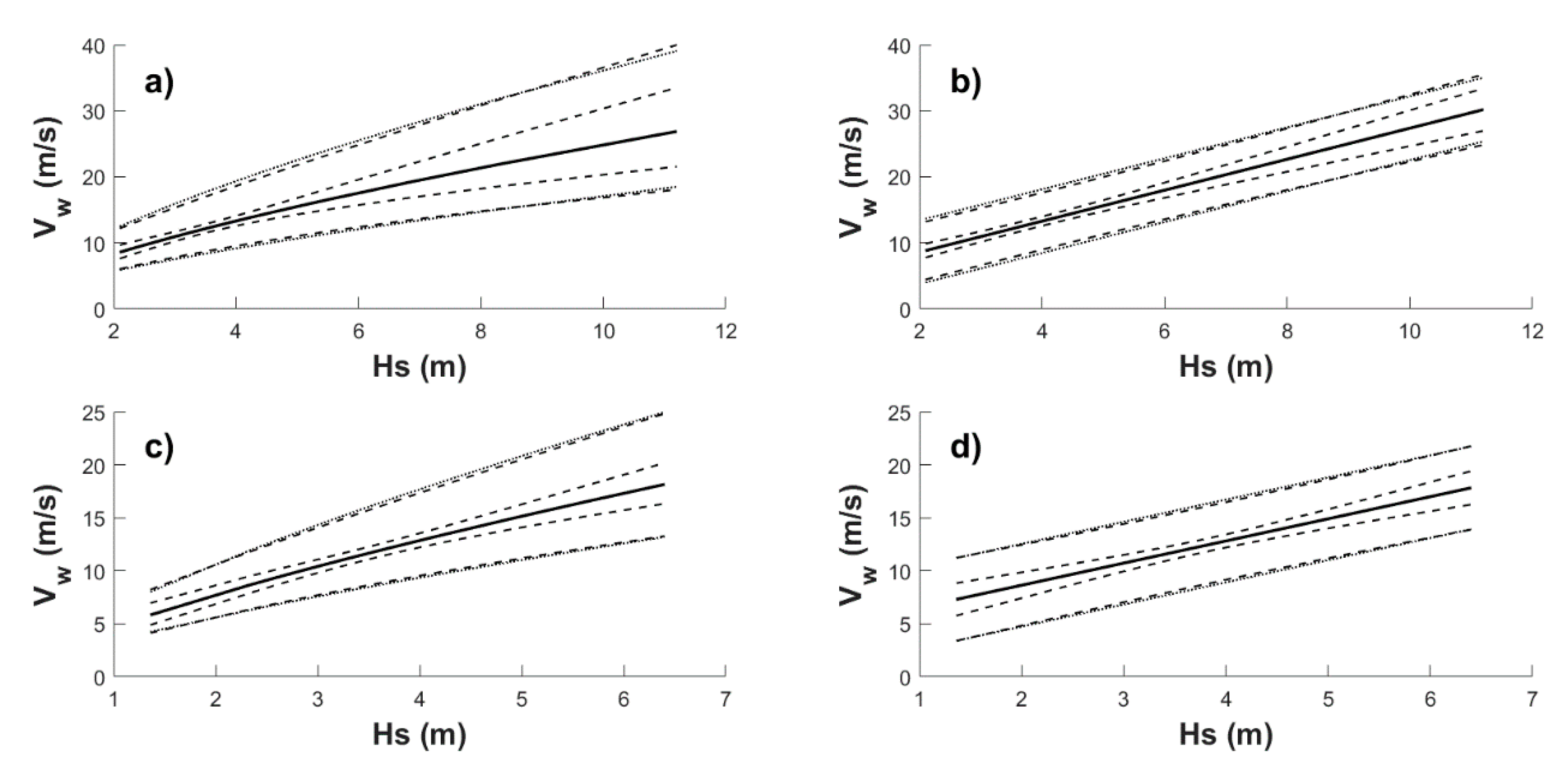
Exact confidence intervals (dashed lines) and approximated confidence intervals (Equations (11) or (12); dotted lines) are shown in Figure 6a–d for the four cases depicted in Figure 3a,b and Figure 5a,b, respectively; the original instead of the logarithmic scale is used for the cases corresponding to Equations (8) and (12). A value of δ equal to 2.3 is used for October (Figure 6a,b), while δ = 2.2 is employed for February (Figure 6c,d). It can be observed that Equations (11) and (12) are reasonable alternatives to represent the uncertainty in a simplified (practical) way. Even though simple, as far as the authors know, Equations (11) and (12) are not reported in the literature for extreme values accounting for seasonality; therefore, they are an important contribution of this study that include the uncertainty in correlated metocean variables for design purposes.
The proposed approach to estimate concurrent metocean variables (Hs and Vw in this case), is based on using the time-dependent GEV model for Hs obtained in the previous section, to compute a Hs value associated with a selected return period in years, T-yr (the subscript is used to denote the selected return period, e.g., T-30 corresponds to a 30-yr return period); the Hs for a given T-yr can then be used as input for Equations (8) and (10)–(12), to determine the corresponding expected companion Vw for the same T-yr, including an uncertainty measure (i.e., the confidence intervals).
To investigate whether the previous proposal is consistent with both time-dependent GEV models in the previous section, estimated values of Hs and Vw associated with T-20, T-30, T-50, T-75 and T-100 are included in the scattergrams and regression analyses as can be observed in Figure 7, where the T-yr values for October are indicated by black filled circles with embedded perpendicular lines (lines to be explained below). Selection of these return periods is somewhat arbitrary but based on the usage of such return periods for design.
Figure 7a,b correspond to the logarithmic and linear cases as before, with the regression line depicted with a solid line and confidence intervals with dashed lines (it is emphasized once more that they are derived by including the set of T-yr values from the GEV models in the regression). In fact, the regression lines and confidence intervals previously obtained (i.e., without including the black filled circles in the regression) are also plotted in Figure 7a,b using dashed–dotted and dotted lines, respectively. It can be observed that the regression lines are almost coincidental, that the estimated T-yr values are very near or over the regression line (especially for Figure 7b), and that the inclusion of T-yr values in the regression slightly decreases the uncertainty in terms of confidence intervals (i.e., the previously computed intervals are wider), which applies to both, Figure 7a,b.
Additionally, the amplitude between the lower and upper limits of the 95% confidence intervals from the GEV models for Hs and Vw are depicted with the perpendicular embedded lines in the T-yr values (i.e., embedded lines in the black filled circles) in Figure 7; vertical and horizontal embedded lines correspond to the confidence intervals for Vw and Hs, respectively. The confidence intervals from the GEV models (the embedded lines in Figure 7) are obtained by using return period values (Equation (6)) and their variance, linked to the variance–covariance matrix and obtained through the delta method [29]. It can be observed in Figure 7a,b that confidence intervals from the GEV models surpass the limits of the confidence intervals for mean values (inner dashed and dotted lines) but are contained within the boundaries of those corresponding to future values (outer dashed and dotted lines) from the regression analysis; it can also be observed that intervals for Hs are wider than for Vw. If it were of interest to delimit in a simplified way the confidence intervals from the GEV models for a given T-yr, Equations (11) and (12) could be an option by providing a suitable δ value. Neither this comparison between the uncertainty of the GEV models and the uncertainty from the linear regression, nor the idea of using Equations (11) and (12) to relate both uncertainties, are found in the literature. Therefore, this can be also considered as a contribution of the present study.
Figure 8 shows the residuals and normal probability papers by including the T-yr values in the regression, where the residuals of T-yr values lie very close to or on the zero-mean line, and the probability papers preserve roughly similar trends than without considering the T-yr values and follow an approximately normal distribution.
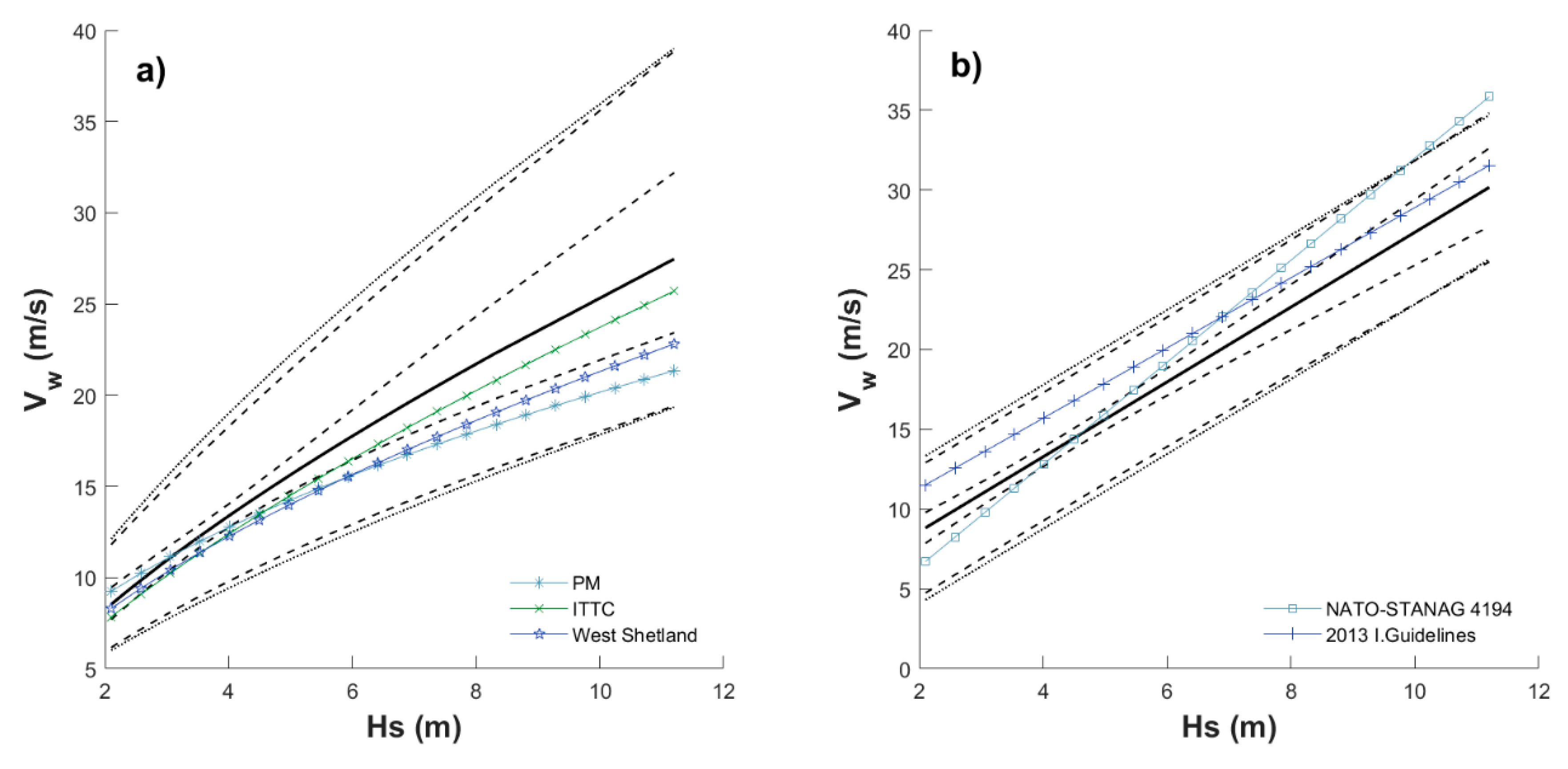
Figure 9a,b is analogous to Figure 6a,b and they are comparable, as can be observed in these figures, with slightly less wider confidence intervals in Figure 9; as in Figure 6 for October, δ = 2.3 is also used in Figure 9. For illustration purposes, the expression of Pierson–Moskowitz (PM), the one from the International Towing Tank Conference (ITTC) recommendations and a fitted equation for West Shetland at a North Atlantic location, are shown in Figure 9a, and the equations recommended by the NATO-STANAG 4194 and the 2013 Interim Guidelines proposed in MEPC 232 (65) are shown in Figure 9b; all these equations are retrieved from [26], where details and proper citation can be found. Some of these equations are given as a function of Vw instead of Hs [26]; in such cases, equations are solved for Vw as a function of Hs. The PM, ITTC and West Shetland expressions have the functional form of Equation (8) with values of b equal to 6.376, 4.636 and 5.31, respectively, and values of α equal to 0.5, 0.709 and 0.603, respectively. Likewise, for the NATO-STANAG and 2013 Interim Guidelines, the corresponding functional form is given by Equation (10) with parameters b equal to 0 and 6.9 and α equal to 3.2 and 2.2, respectively. For the previous expressions Hs is given in m and Vw in m/s. Note that the NATO-STANAG and 2013 Interim Guidelines equations are developed for coastal waters but included in Figure 9b for comparison. Figure 9 shows that the ITTC and the 2013 Interim Guidelines equations are similar in shape to those developed in this study, but under- or overestimating the predicted values for October the former and the latter, respectively. The other equations lead to not so dissimilar results as those reported here, and they are roughly in between the confidence intervals for future values.
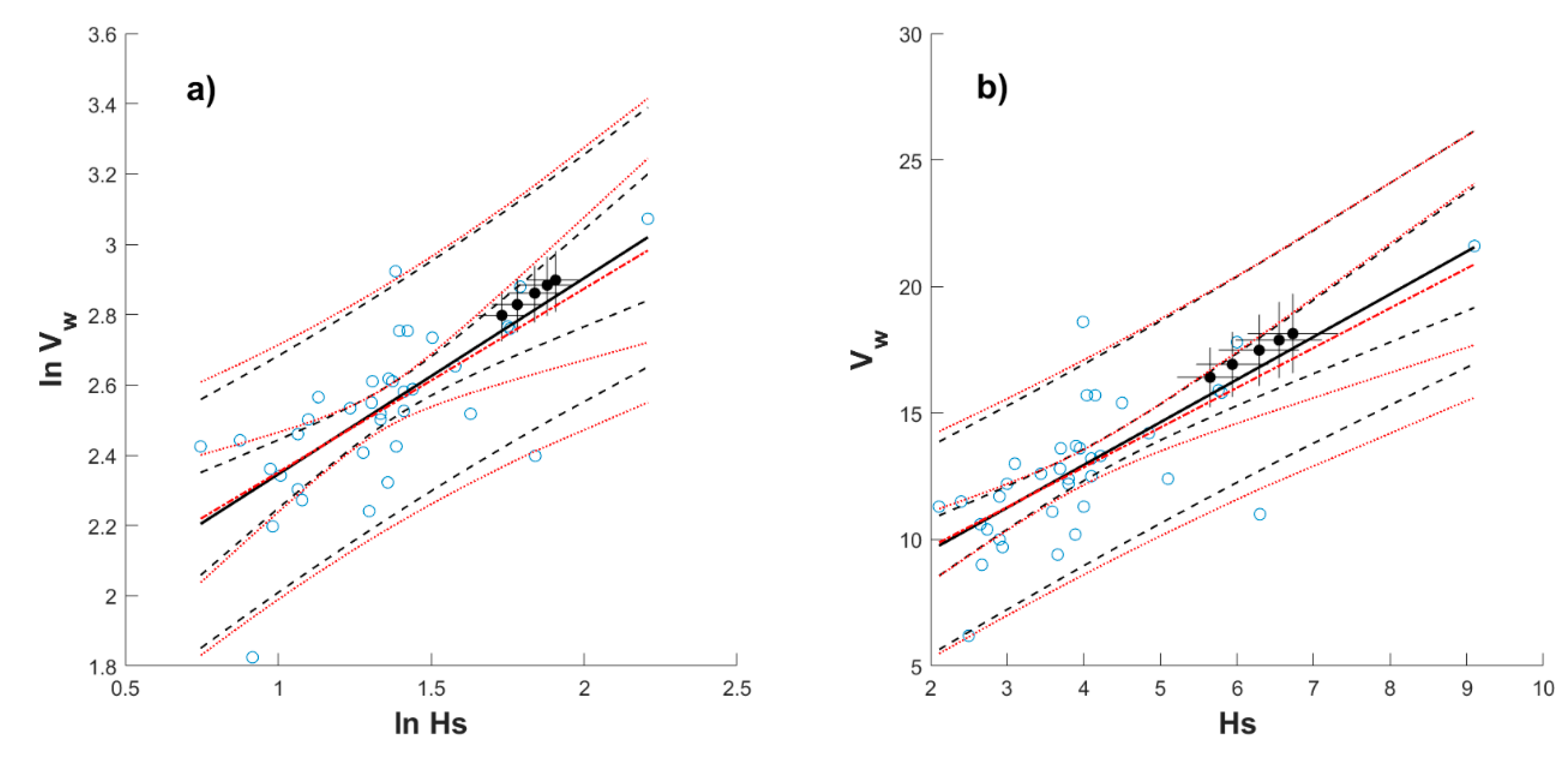
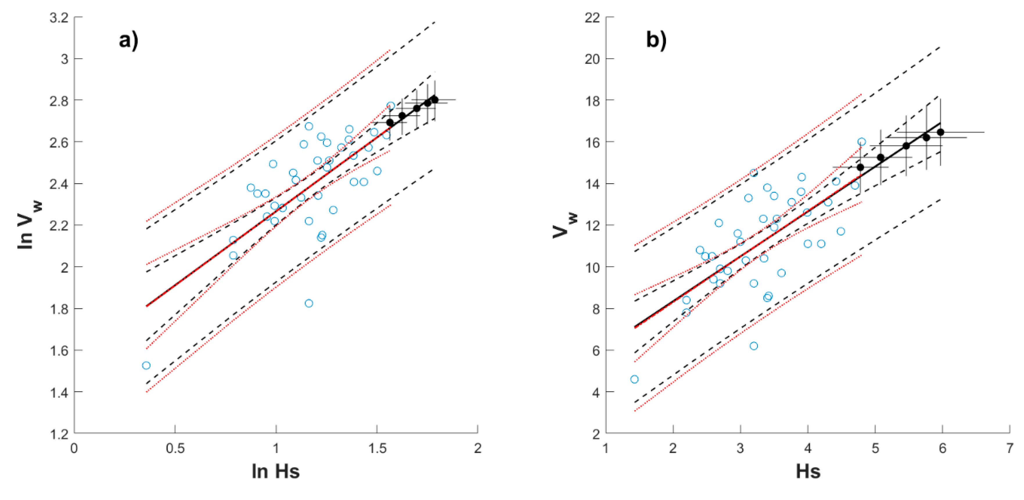
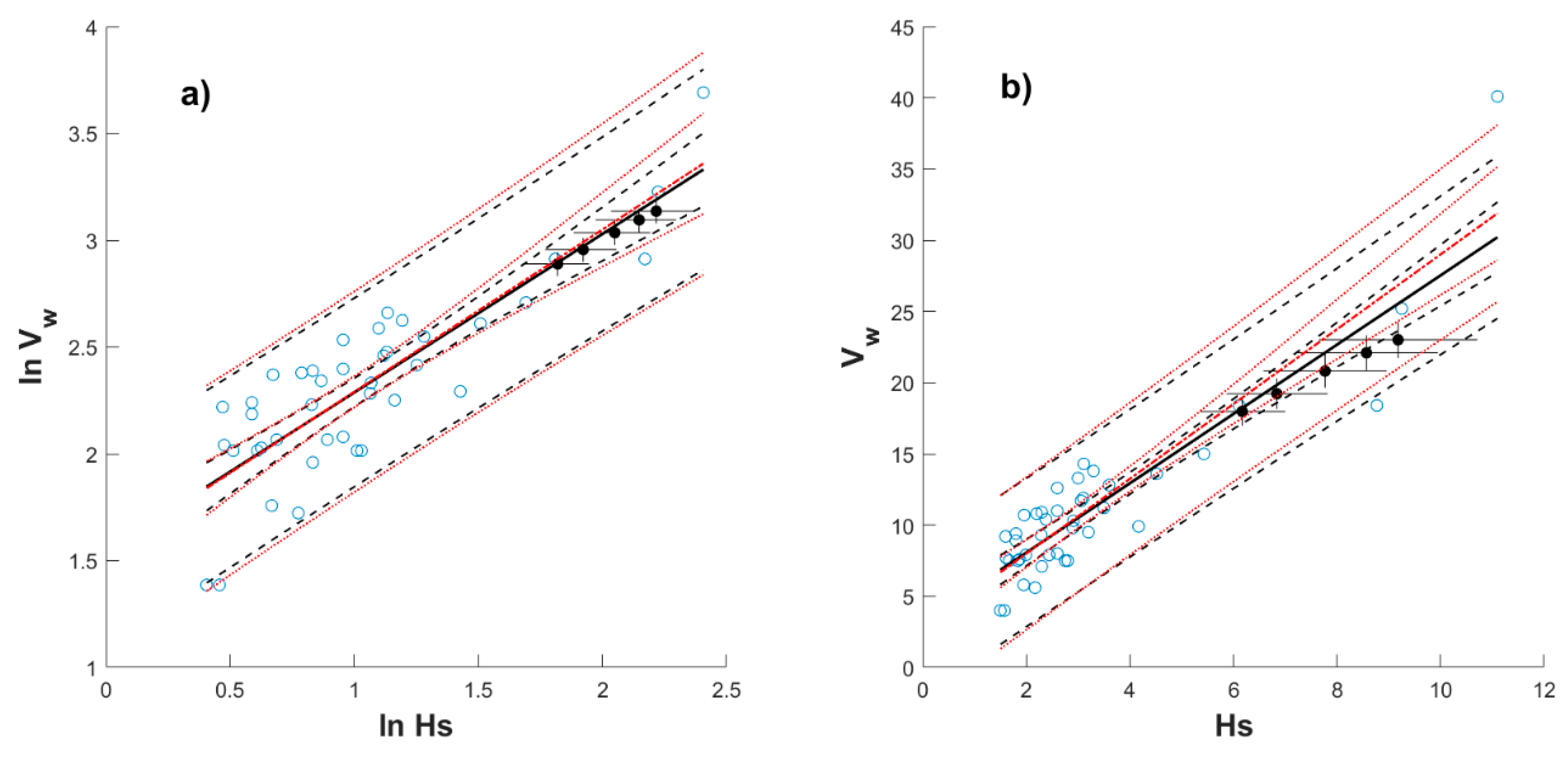
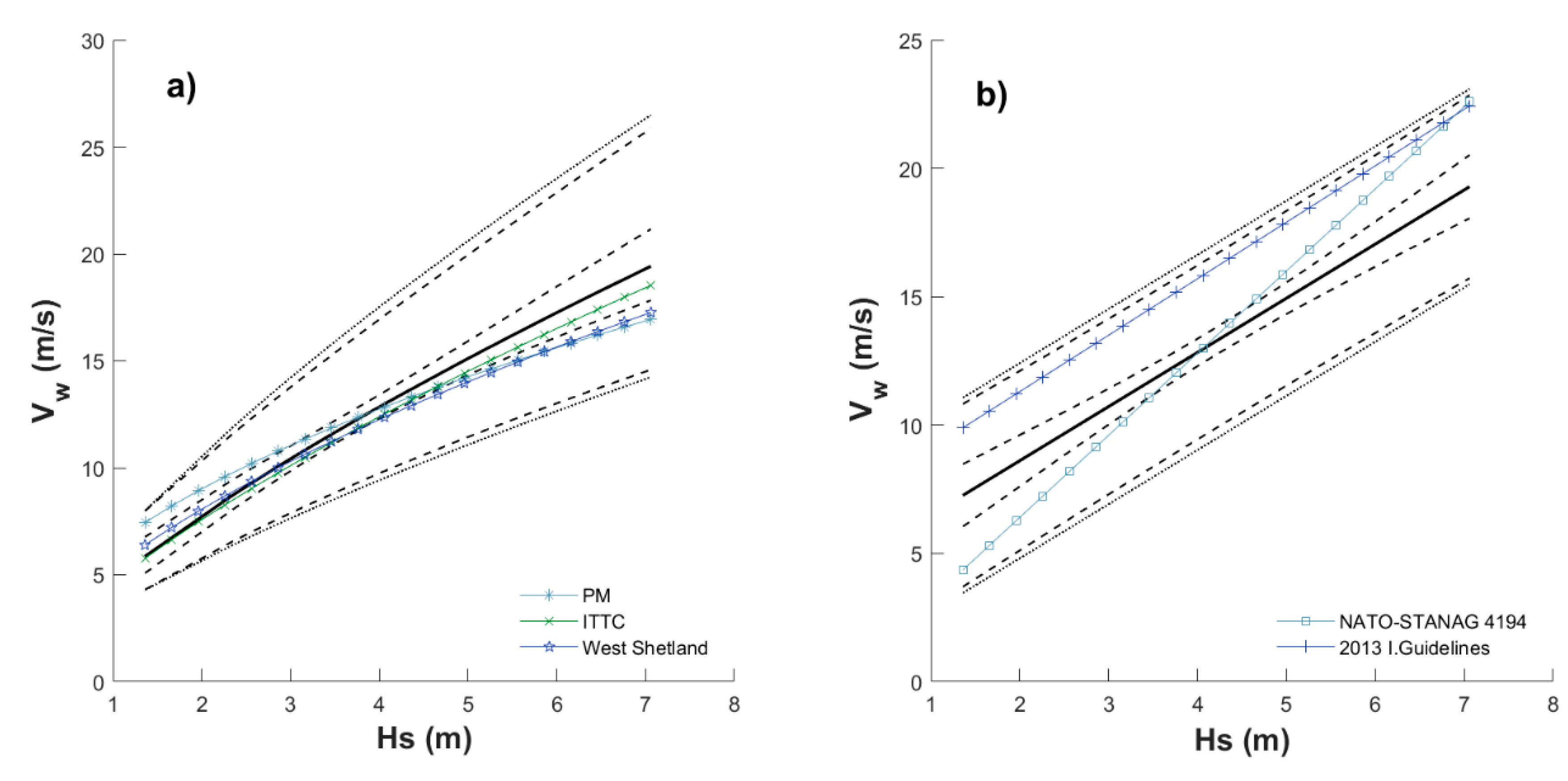
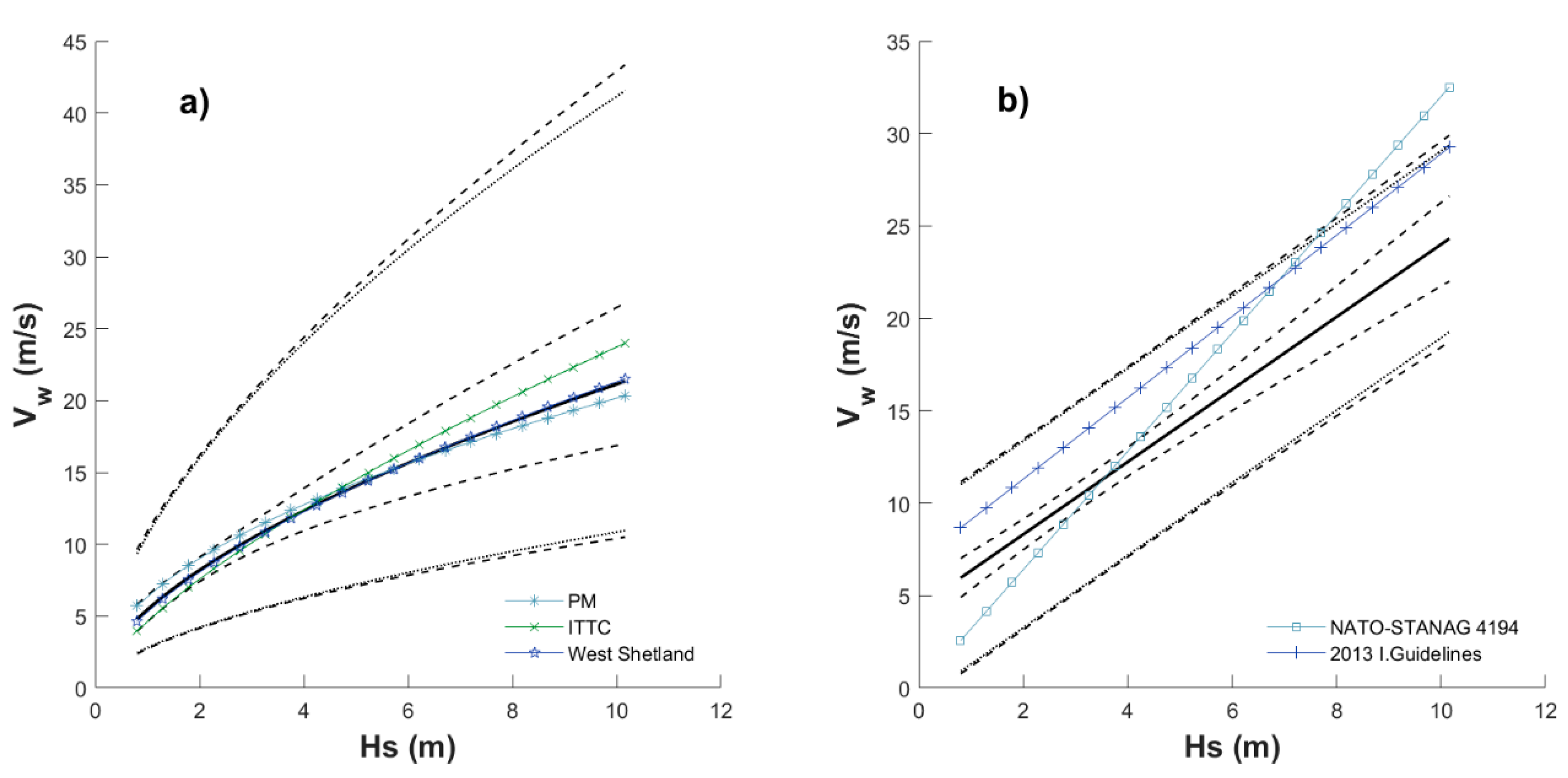
To inspect how the proposed approach varies when considering seasonality, and how results compare with respect to the equations reported in [26] for other seasons, results like those shown in Figure 7 are also shown in Figure 10 and Figure 11, but for the months of February and August, when the highest predicted T-yr values are obtained at cold front and hurricane seasons, respectively; in addition, results like those in Figure 9 are plotted in Figure 12 and Figure 13. Unlike Figure 9, δ = 2.0 is used in Figure 12 and Figure 13, since it leads to a better approximation of the exact confidence intervals. As mentioned before, δ can be varied to better represent the exact confidence intervals; nevertheless, the range of values is not large and δ can be roughly set between 1.9 and 2.3.
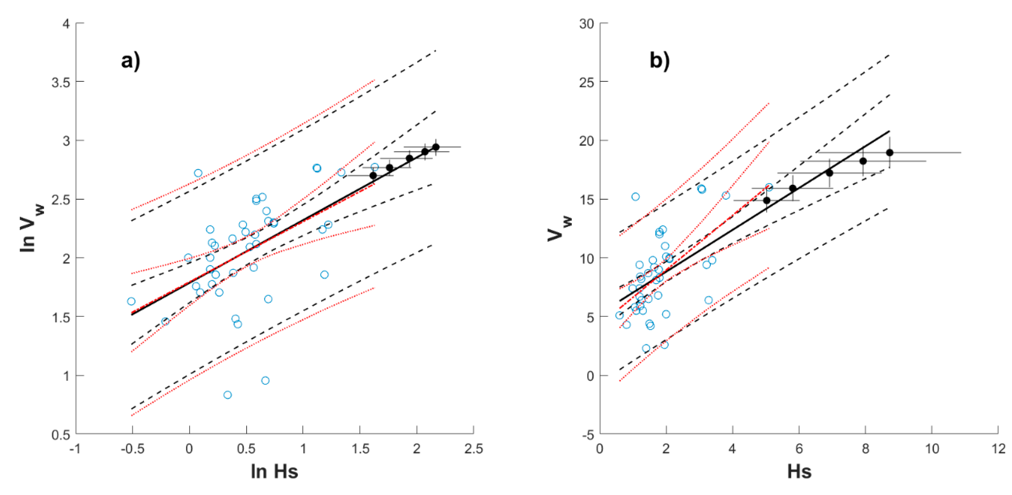
It can be observed from Figure 7, Figure 10 and Figure 11 that expected Vw values as function of Hs depend on the season and month considered, that the uncertainty also varies for each case and that the regression is relatively irrespective of the selected scheme (linear or logarithmic space) for October and February, but it does vary when August is considered. Figure 11 for August corresponds to the largest estimated T-yr values for Hs (hurricane season) and, as shown in Figure 11, the regression line predicts better estimates when the regression is performed in the logarithmic space; in fact, when the T-yr values are included in the regression (solid line), there is not significant deviation from the regression with the observed data only (dashed–dotted line); conversely, an important change in the slope of the regression line is observed for Figure 11b, implying better estimates of correlated values for given T-yr if the regression is carried out in the logarithmic space.
Figure 9, Figure 12 and Figure 13 show that a single equation cannot capture the seasonality of correlated metocean variables, because it can overestimate or underestimate the correlated values when comparing against the equations compiled in [26], at least for the case of Vw and Hs and buoy 42001, but it is possibly the case for other metocean variables and buoys, in the Gulf of Mexico or anywhere else. Therefore, suitable sets of region-specific and site-specific equations should be developed to take into account seasonal effects. Nonetheless, it is interesting to note that the equation developed in [26] for West Shetland is practically coincident with the regression line in Figure 13a at hurricane season.
For values associated with T-yr levels in Figure 11a (or in other figures), the uncertainty from the GEV models for each T-yr (i.e., the embedded perpendicular lines in the black filled circles) are a sort of envelope roughly covered by the confidence intervals for mean values in Figure 11a. Furthermore, such an envelope can be covered by using Equation (12) and a smaller value of δ (e.g., δ = 1) than that used for the confidence intervals of future values. Therefore, Equations (8) and (10) can be considered as possible design aids—simple expressions for design—like those contained in guidelines [26], but also accounting for the uncertainty in a simplified way (Equations (11) and (12)), either based on simplified confidence intervals for future values or confidence intervals within which the GEV uncertainty is confined. Since sets of such equations can be obtained for any desired season, the proposal here represents a simpler alternative than the more complex models reported in the introduction; consequently, they could be more attractive for designers since they are consistent with expressions recommended in guidelines.
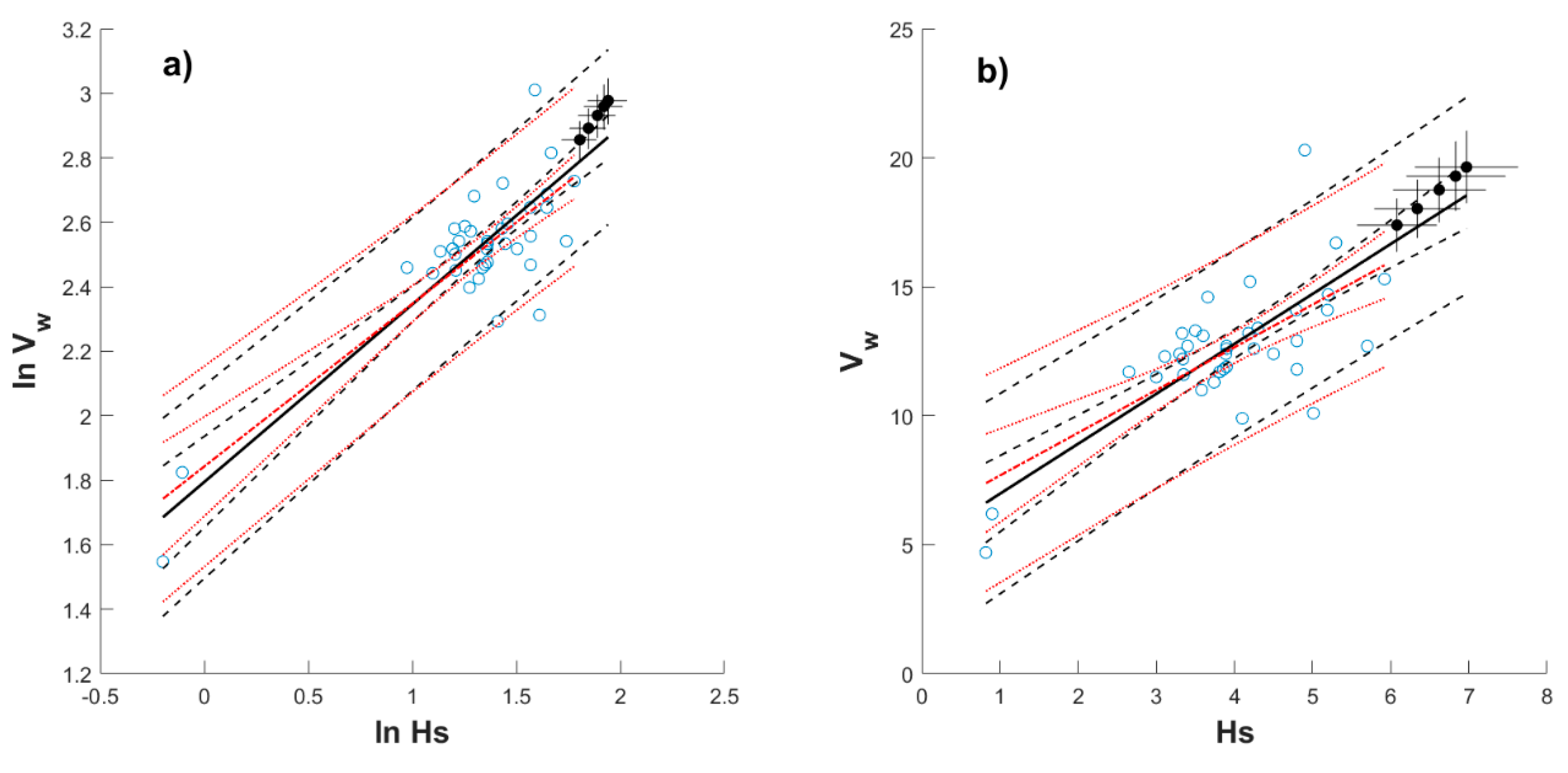
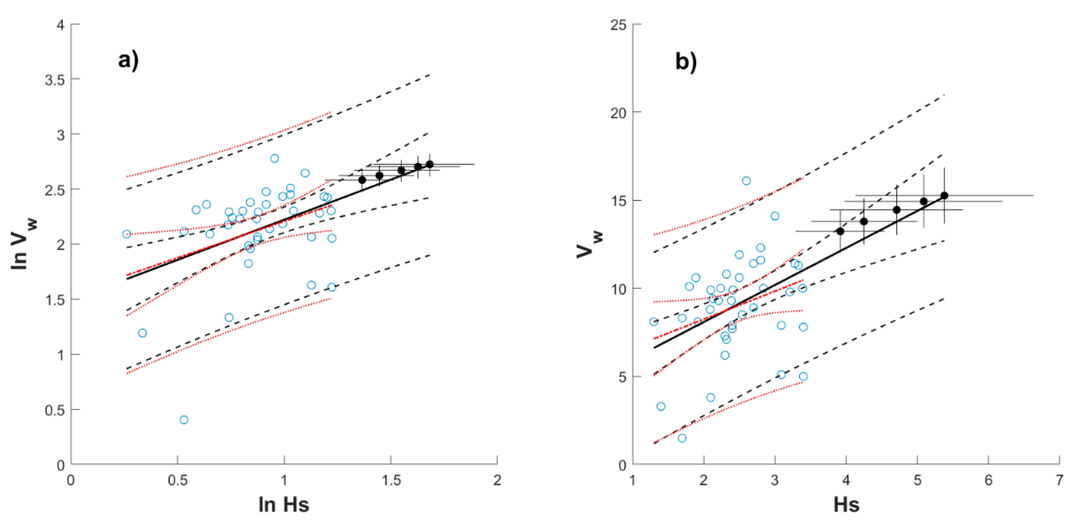
Results for other months (not shown before) are reported in Figure A1, Figure A2, Figure A3, Figure A4, Figure A5, Figure A6, Figure A7, Figure A8 and Figure A9 in Appendix B. By observing Figure 7, Figure 10 and Figure 11 and Figure A1, Figure A2, Figure A3, Figure A4, Figure A5, Figure A6, Figure A7, Figure A8 and Figure A9, it can be concluded that the regression in the logarithmic or linear space could be both alternatives, with better results depending on the month considered. An exception is shown by Figure A8 for November, where neither a good fit is obtained for the logarithmic case (Figure A8a) nor for the linear one (Figure A8b) (also see Table 1). This is attributed to atypical simultaneous occurrence of larger Hs and smaller Vw values, as can be observed in Figure A8, but also to a large dispersion of the data along the whole range of Hs values, leading to a regression line somewhat horizontal (and roughly around 12 m/s), implying no correlation of Hs and Vw for November. It would be interesting to investigate in the future why this behavior is found specifically for November at buoy 42,001 in the Gulf of Mexico. For all the residual analyses shown in Figure 7, Figure 10 and Figure 11, and Figure A1, Figure A2, Figure A3, Figure A4, Figure A5, Figure A6, Figure A7, Figure A8 and Figure A9 for the observed data, mean values of these residuals are listed in Table A3 of Appendix C. In general, it can be observed in Table A3 that the zero mean assumption is met.
Results of the regression are listed for each month in Table 1 for buoy 42,001. Table 1 includes the regression parameters using only the observed data and the two approaches described above, i.e., the direct linear regression and the regression in the logarithmic space. It also includes σe and relative errors of the predicted correlated Vw in relation to those obtained from the GEV model for a selected return period (50 years) using:
ε V = | V b e n c h V e s t V b e n c h | × 100
where the relative error is given in percentage, Vbench is the computed T-50 value of Vw using the GEV model and Vest is obtained as proposed in this study, i.e., by using Hs for T-50 obtained from the GEV model as input value of Equations (8) and (10) (with regression parameters estimated from observed data only). Selection of T-50 is somewhat arbitrary and used to compare deviations of Vw estimated with the GEV model with respect to this study’s proposal, but any other T-yr could be considered. For a more detailed inspection of these deviations, Figure 7, Figure 10 and Figure 11 and those in the Appendix B can be used. Errors in Table 1 are an additional aid to compare which regression scheme leads to better results for any given month.
The proposal in this study can be summarized in the following steps:
(1)
Select an Hs value associated with a T-yr and month of interest (e.g., see Table A1 in Appendix A) as input for Equations (8) or (10).
(2)
Select the season (month) for which the correlated values are desired, and the corresponding parameters (Table 1) to be also plugged into Equation (8) or (10), and compute Vw.
(3)
Use Hs in step (1) and Vw in step (2) as simultaneous demands associated with the selected T-yr and month acting over a maritime system to be designed.
(4)
If uncertainty is to be used by the designer, the corresponding σe together with Equations (11) or (12) can be used to establish upper (or lower) limits by using a δ value (e.g., δ = 2 could be used to approximate the 95% confidence intervals for future values).

5. Discussion

For the proposal briefly outlined in the four steps of the previous section, it is noted that for step (1) the T-yr values of Hs are related to the GEV model, but any projected return level of the significant wave height available to the designer could be useful, at least as an approximation. Also, since for any given month selected, two options are available in step (2), namely, Equation (8) or Equation (10), the decision for the more suitable option can be based on the εV reported in Table 1, as well as on Figure 7, Figure 10 and Figure 11 and Figure A1, Figure A2, Figure A3, Figure A4, Figure A5, Figure A6, Figure A7, Figure A8 and Figure A9. Justification for considering Hs and Vw for T-yr in step (3) as simultaneously occurring metocean variables is based not only on the correlation of recorded (observed) data, but also in checking that the correlation of projected Hs and Vw for T-yr, obtained from the time-dependent GEV models, are consistent with the trend of the observed data. Finally, the uncertainty obtained as per Equations (11) or (12) in step (4) approximately delimits all data points if δ = 2 is used (confidence intervals for future values); if the uncertainty from the GEV models is to be employed as reference (perhaps considering the perpendicular embedded lines as an envelope), lower δ values could be used, for instance δ = 1.5, which would be a conservative value to delimit the uncertainty given by the GEV models. Use of Equations (11) or (12) using δ values could be seen as factored demands like the ones used in codified design.
The proposed method allows the possibility of using other metocean variables, data from other buoys and hindcast data. It could use other probabilistic models. More than two variables could be considered if multilinear regression analysis is implemented. If additional recorded data becomes available for any month, the matrix approach in [35] can be implemented to update the parameters in Table 1.
Since the maximum Hs and companion Vw may not yield the maximum demand in a given system—like the points in an environmental contour associated with a T-yr may not lead to the maximum demand in the system [20]—other pairs of simultaneously recorded data could be considered; one obvious combination is using maximum monthly Vw and companion Hs, but also other data pairs could be used, for instance the second largest monthly Hs and companion Vw, the second largest Vw and companion Hs, the third largest monthly Hs and companion Vw and so on. Each of the previous combinations would lead to pairs of T-yr values to which a system could be subjected to for estimating load effects, and the maximum demand could be used for design (in fact, different pairs of T-yr values could be more critical to different elements of the system). It could be investigated whether these pairs of T-yr values correspond to points of environmental contours proposed by other authors. Nonetheless, the idea is consistent with the approach of using multiple points from the contours to evaluate a system [20].

6. Conclusions

In this study, a simplified methodology to compute maximum significant wave heights and companion wind velocities associated with given return periods, accounting for seasonality, is presented. Simultaneous data from a buoy in the Gulf of Mexico are used. The approach is developed from projected return levels of significant wave heights based on a time-dependent GEV model and classical regression of the two metocean variables. A time-dependent GEV model for the companion wind velocities is also developed, to assess the adequacy of the method to predict the wind velocity as a function of significant wave height for a given return period.
It is found that the time window selected to estimate return period values of metocean variables can have an important impact in the predicted return levels for some seasons.
It is concluded that correlation of significant weight height and companion wind velocity can be adequately represented by linear or power equations, which could be easily implemented for design purposes, with different parameters to account for seasonality, but with the same functional form. Results are not very dissimilar with predictions from simplified equations in the literature or guidelines; however, it is found that a single equation with given parameters cannot capture the seasonality effects.
It is also found that the uncertainty in the predicted companion wind velocities as a function of significant wave height can be determined in a simplified way by using the root mean squared error from the regression analysis, expressed as a set of proposed equations to determine approximately (but closely) the 95% confidence intervals of future values. These same equations can be used to represent the envelope of the uncertainty estimated from the GEV models for different return periods.
It is considered that the proposed approach is a simple but adequate method to determine concurrent metocean hazards associated with given return periods, which could be imposed on a system to estimate the demand for design purposes, while also providing measures of uncertainty. The proposed expressions do not differ substantially to those provided in guidelines; thus, they could be amenable to designers, while also incorporating the seasonality effects in a simpler way as compared to other methods available in the literature. To the authors’ knowledge, some of the findings in the present study—like the simplified proposal to include the uncertainty in the correlated metocean variables—are not reported elsewhere.

Author Contributions

Conceptualization, F.C.-V., A.-D.G.-S. and C.M.; Formal analysis, F.C.-V., A.-D.G.-S. and C.M.; Funding acquisition, A.-D.G.-S. and C.M.; Investigation, F.C.-V., A.-D.G.-S. and C.M.; Methodology, F.C.-V., A.-D.G.-S and C.M.; Project administration, C.M.; Supervision, A.-D.G.-S. and C.M. All authors have read and agreed to the published version of the manuscript.

Funding

The financial support from the Erasmus Mundus Coastal and Marine Engineering and Management (CoMEM) programme and support from Laboratori d’Enginyeria Marítima, Universitat Politècnica de Catalunya and from Universidad de Guanajuato (CIIC 2020 Research Projects) is gratefully acknowledged.

Acknowledgments

We thank two anonymous reviewers for their comments, suggestions and constructive criticism. We also thank guess Editor Guido Ventura and the editorial team of Applied Sciences for their help in the editorial process.

Conflicts of Interest

The authors declare no conflict of interest.

Appendix A

Table A1. Selected return period values for Hs in each month.
Hs (m)
Month\Tr (yr)20305075100
January6.086.346.626.836.97
February6.096.366.686.917.06
March5.655.946.296.556.73
April4.785.085.465.765.97
May3.924.254.715.095.38
June4.034.535.255.886.36
July5.035.816.927.938.73
August5.996.878.139.2710.16
September6.176.847.778.579.18
October5.906.336.887.347.67
November5.766.056.416.696.88
December5.896.146.436.646.78
Table A2. Selected return period values for Vw in each month.
Vw (m/s)
Month\Tr (yr)20305075100
January17.3918.0318.7619.2919.64
February17.3617.9218.5519.0019.29
March16.4116.9217.4817.8818.14
April14.7715.2515.8016.2016.46
May13.2313.7914.4514.9315.26
June13.3014.0614.9715.6616.14
July14.8815.9217.2218.2318.95
August16.8818.1419.7521.0321.95
September17.9819.2220.8122.0923.01
October17.7118.7420.0521.0921.83
November17.1517.9919.0119.8120.37
December17.0817.7918.6219.2519.68

Appendix B

Figure A1. Regression lines and confidence intervals including (solid and dashed lines, respectively) and excluding (dashed–dotted and dotted lines, respectively) T-yr values for January; (a) and (b) for logarithmic space and linear space, respectively. Filled circles represent T-yr values with embedded perpendicular lines indicating confidence intervals from GEV models.
Applsci 10 04794 g0a1
Figure A2. Regression lines and confidence intervals including (solid and dashed lines, respectively) and excluding (dashed–dotted and dotted lines, respectively) T-yr values for March; (a) and (b) for logarithmic space and linear space, respectively. Filled circles represent T-yr values with embedded perpendicular lines indicating confidence intervals from GEV models.
Applsci 10 04794 g0a2
Figure A3. Regression lines and confidence intervals including (solid and dashed lines, respectively) and excluding (dashed–dotted and dotted lines, respectively) T-yr values for April; (a) and (b) for logarithmic space and linear space, respectively. Filled circles represent T-yr values with embedded perpendicular lines indicating confidence intervals from GEV models.
Applsci 10 04794 g0a3
Figure A4. Regression lines and confidence intervals including (solid and dashed lines, respectively) and excluding (dashed–dotted and dotted lines, respectively) T-yr values for May; (a) and (b) for logarithmic space and linear space, respectively. Filled circles represent T-yr values with embedded perpendicular lines indicating confidence intervals from GEV models.
Applsci 10 04794 g0a4
Figure A5. Regression lines and confidence intervals including (solid and dashed lines, respectively) and excluding (dashed–dotted and dotted lines, respectively) T-yr values for June; (a) and (b) for logarithmic space and linear space, respectively. Filled circles represent T-yr values with embedded perpendicular lines indicating confidence intervals from GEV models.
Applsci 10 04794 g0a5
Figure A6. Regression lines and confidence intervals including (solid and dashed lines, respectively) and excluding (dashed–dotted and dotted lines, respectively) T-yr values for July; (a) and (b) for logarithmic space and linear space, respectively. Filled circles represent T-yr values with embedded perpendicular lines indicating confidence intervals from GEV models.
Applsci 10 04794 g0a6
Figure A7. Regression lines and confidence intervals including (solid and dashed lines, respectively) and excluding (dashed–dotted and dotted lines, respectively) T-yr values for September; (a) and (b) for logarithmic space and linear space, respectively. Filled circles represent T-yr values with embedded perpendicular lines indicating confidence intervals from GEV models.
Applsci 10 04794 g0a7
Figure A8. Regression lines and confidence intervals including (solid and dashed lines, respectively) and excluding (dashed–dotted and dotted lines, respectively) T-yr values for November; (a) and (b) for logarithmic space and linear space, respectively. Filled circles represent T-yr values with embedded perpendicular lines indicating confidence intervals from GEV models.
Applsci 10 04794 g0a8
Figure A9. Regression lines and confidence intervals including (solid and dashed lines, respectively) and excluding (dashed–dotted and dotted lines, respectively) T-yr values for December; (a) and (b) for logarithmic space and linear space, respectively. Filled circles represent T-yr values with embedded perpendicular lines indicating confidence intervals from GEV models.
Applsci 10 04794 g0a9

Appendix C

Table A3. Mean values of residuals for each month and regression scheme.
MonthLog. SpaceLin. Space
January7.8 × 10−17–4.5 × 10⁻¹⁶
February3.4 × 10−161.9 × 10⁻¹⁵
March–5.1 × 10−161.4 × 10⁻¹⁵
April1.8 × 10−171.4 × 10⁻¹⁵
May–3.3 × 10−169.1 × 10⁻¹⁷
June4.8 × 10−17–1.3 × 10⁻¹⁵
July1.4 × 10−168.9 × 10⁻¹⁶
August4.3 × 10−16–3.2 × 10⁻¹⁵
September–4.4 × 10−169.5 × 10⁻¹⁶
October0.08.9 × 10−16
November9.9 × 10−17–1.4 × 10⁻¹⁵
December–5.6 × 10⁻¹⁷–2.4 × 10⁻¹⁶

References

  1. Castillo, E.; Hadi, A.S.; Balakrishnan, N.; Sarabia, J.M. Extreme Value and Related Models with Applications in Engineering and Science; Wiley: Hoboken, NJ, USA, 2004; Volume 4, pp. 1–362. [Google Scholar]
  2. Hong, H.P. Estimate of extreme wind and wave loading and safety level of offshore structures. In Proceedings of the Risk Analysis: Proceedings of a Symposium, Ann Arbor, MI, USA, 11–12 August 1994; University of Michigan: Ann Arbor, MI, USA, 1994; Volume 4, pp. 107–117. [Google Scholar]
  3. Nessim, M.A.; Hong, H.P.; Swail, V.R.; Henderson, C.A. Design criteria for offshore structures under combined wind and wave loading. J. Offshore Mech. Arct. Eng. 1995, 117, 1–11. [Google Scholar] [CrossRef]
  4. Shao, Z.; Liang, B.; Li, H.; Lee, D. Study of sampling methods for assessment of extreme significant wave heights in the South China Sea. Ocean Eng. 2018, 168, 173. [Google Scholar] [CrossRef]
  5. Shao, Z.; Liang, B.; Li, H.; Wu, G.; Wu, Z. Blended wind fields for wave modeling of tropical cyclones in the the South China Sea and East China Sea. Appl. Ocean Res. 2018, 71, 20. [Google Scholar] [CrossRef]
  6. Ludeno, G.; Serafino, F. Estimation of the Significant Wave Height from Marine Radar Images without External Reference. J. Mar. Sci. Eng. 2019, 7, 432. [Google Scholar] [CrossRef] [Green Version]
  7. Chen, S.-T.; Wang, Y.-W. Improving Coastal Ocean Wave Height Forecasting during Typhoons by using Local Meteorological and Neighboring Wave Data in Support Vector Regression Models. J. Mar. Sci. Eng. 2020, 8, 149. [Google Scholar] [CrossRef] [Green Version]
  8. Gao, H.; Shao, Z.; Wu, G.; Li, P. Study of Directional Declustering for Estimating Extreme Wave Heights in the Yellow Sea. J. Mar. Sci. Eng. 2020, 8, 236. [Google Scholar] [CrossRef] [Green Version]
  9. Katalinić, M.; Parunov, J. Uncertainties of Estimating Extreme Significant Wave Height for Engineering Applications Depending on the Approach and Fitting Technique—Adriatic Sea Case Study. J. Mar. Sci. Eng. 2020, 8, 259. [Google Scholar] [CrossRef] [Green Version]
  10. Cavaleri, L.; Barbariol, F.; Benetazzo, A. Wind–Wave Modeling: Where We Are, Where to Go. J. Mar. Sci. Eng. 2020, 8, 260. [Google Scholar] [CrossRef] [Green Version]
  11. Weisse, R.; Gaslikova, L.; Geyer, B.; Groll, N.; Meyer, E. Coastdat—Model data for science and industry. Kuste Westholsteinische Verl. Boyens Co. 2014, 81, 5–18. [Google Scholar]
  12. Weisse, R.; Groll, N. A multi-decadal wind-wave hindcast for the North Sea 1949–2014: CoastDat2. Earth Syst. Sci. Data 2017, 9, 955. [Google Scholar]
  13. Monish, N.T.; Rehana, S. Suitability of distributions for standard precipitation and evapotranspiration index over meteorologically homogeneous zones of India. J. Earth Syst. Sci. 2020, 129, 25. [Google Scholar] [CrossRef]
  14. Schardong, A.; Simonovic, S.P.; Gaur, A.; Sandink, D. Web-Based Tool for the Development of Intensity Duration Frequency Curves under Changing Climate at Gauged and Ungauged Locations. Water 2020, 12, 1243. [Google Scholar] [CrossRef]
  15. Prakash, A.; Panchang, V.; Ding, Y.; Ntaimo, L. Sign Constrained Bayesian Inference for Nonstationary Models of Extreme Events. J. Waterw. Port Coast. Ocean Eng. ASCE 2020, 146, 04020029. [Google Scholar] [CrossRef]
  16. Kim, H.-J.; Suh, S.-W. Improved Hypothetical Typhoon Generation Technique for Storm Surge Frequency Analyses on the Southwest Korean Coast. J. Coast. Res. 2018, 85, 516. [Google Scholar] [CrossRef]
  17. Weinan, H.; Shanshan, T.; Qiang, B.; Sheng, D. Bivariate Distribution Modelling for Wave Height and Period in Jiaozhou Bay. In Proceedings of the ASME 2018 37th International Conference on Ocean, Offshore and Arctic Engineering 2018, Volume 11B: Honoring Symposium for Professor Carlos Guedes Soares on Marine Technology and Ocean Engineering, Madrid, Spain, 17–22 June 2018. V11BT12A054. [Google Scholar] [CrossRef]
  18. Sartini, L.; Besio, G.; Cassola, F. Spatio-temporal modelling of extreme wave heights in the Mediterranean Sea. Ocean Model. 2017, 117, 52. [Google Scholar] [CrossRef]
  19. Muraleedharan, G.; Lucas, C.; Guedes Soares, C. Regression quantile models for estimating trends in extreme significant wave heights. Ocean Eng. 2016, 118, 204. [Google Scholar] [CrossRef]
  20. Ross, E.; Astrup, O.C.; Bitner-Gregersen, E.; Bunn, N.; Feld, G.; Gouldby, B.; Liu, Y.; Randell, D.; Vanem, E.; Jonathan, P. On environmental contours for marine and coastal design. Ocean Eng. 2020, 195, 1. [Google Scholar] [CrossRef]
  21. Vanem, E. A simple approach to account for seasonality in the description of extreme ocean environments. Mar. Syst. Ocean Technol. 2018, 13, 63. [Google Scholar] [CrossRef]
  22. Randell, D.; Feld, G.; Ewans, K.; Jonathan, P. Distributions of return values for the ocean wave characteristics in the South China Sea using directional-seasonal extreme value analysis. Environmetrics 2015, 26, 442. [Google Scholar] [CrossRef]
  23. Randell, D.; Turnbull, K.; Ewans, K.; Jonathan, P. Bayesian inference for nonstationary marginal extremes. Environmetrics 2016, 27, 439. [Google Scholar] [CrossRef] [Green Version]
  24. Ross, E.; Randell, D.; Ewans, K.; Feld, G.; Jonathan, P. Efficient estimation of return value distributions from non-stationary marginal extreme value models using Bayesian inference. Ocean Eng. 2017, 142, 315. [Google Scholar] [CrossRef]
  25. Anokhin, V.; Randell, D.; Ross, E.; Jonathan, P. Spatial and seasonal variability of metocean design criteria in the southern south China Sea from covariate extreme value analysis. In Proceedings of the ASME 2019 38th International Conference on Ocean, Offshore and Artic Engineering, OMAE, Glasgow, Scotland, UK, 9–14 June 2019; Volume 1. [Google Scholar]
  26. Bitner-Gregersen, E.M. Comparison of wind and wave climate in open sea and coastal waters. Ocean Eng. 2018, 170, 199. [Google Scholar] [CrossRef]
  27. National Data Buoy Center (NDBC). Available online: www.ndbc.noaa.gov (accessed on 30 June 2020).
  28. Calderón-Vega, F.; Vázquez-Hernández, A.O.; García-Soto, A.D. Analysis of extreme waves with seasonal variation in the Gulf of Mexico using a time-dependent GEV model. Ocean Eng. 2013, 73, 68–82. [Google Scholar] [CrossRef]
  29. Coles, S.G. An Introduction to Statistical Modelling of Extreme Values, 1st ed.; Springer: London, UK, 2001; Volume 4, pp. 1–208. [Google Scholar]
  30. Calderón Vega, F. Caracterización del Régimen Extremal del Oleaje en el Golfo de México Considerando la Variación Estacional. Master’s Thesis, Universidad de Cantabria, Santander, Spain, 2009. (In Spanish). [Google Scholar]
  31. Bitner-Gregersen, E.M.; Gramstad, O. Potential Changes in the Joint Probabilistic Description of the North Atlantic Wave Climate. In Proceedings of the ASME 2018 37th International Conference on Ocean, Offshore and Arctic Engineering, Volume 11B: Honoring Symposium for Professor Carlos Guedes Soares on Marine Technology and Ocean Engineering, Madrid, Spain, 17–22 June 2018. V11BT12A056. [Google Scholar] [CrossRef]
  32. Hong, H.P.; Zimmerman, T.J.; Bach, L. Probabilistic basis of resistance factors for use in oriented strand board. In Proceedings of the 1st Structural Specialty Conference, Canadian Society of Civil Engineering, Edmonton, AB, Canada, 29 May–1 June 1996; pp. 1223–1235. [Google Scholar]
  33. Jordaan, I. Decisions under Uncertainty: Probabilistic Analysis for Engineering Decisions, 1st ed.; Cambridge University Press: Cambridge, UK, 2005; pp. 1–672. [Google Scholar]
  34. Kottegoda, N.T.; Rosso, R. Applied Statistics for Civil and Environmental Engineers, 2nd ed.; Blackwell Publishing-Wiley: Oxford, UK, 2008; pp. 1–718. [Google Scholar]
  35. Faber, M.H. Statistics and Probability Theory: In Pursuit of Engineering Decision Support, 2nd ed.; Springer: Dordrecht, The Netherlands; Heidelberg, Germany; London, UK; New York, NY, USA, 2012; pp. 1–190. [Google Scholar]
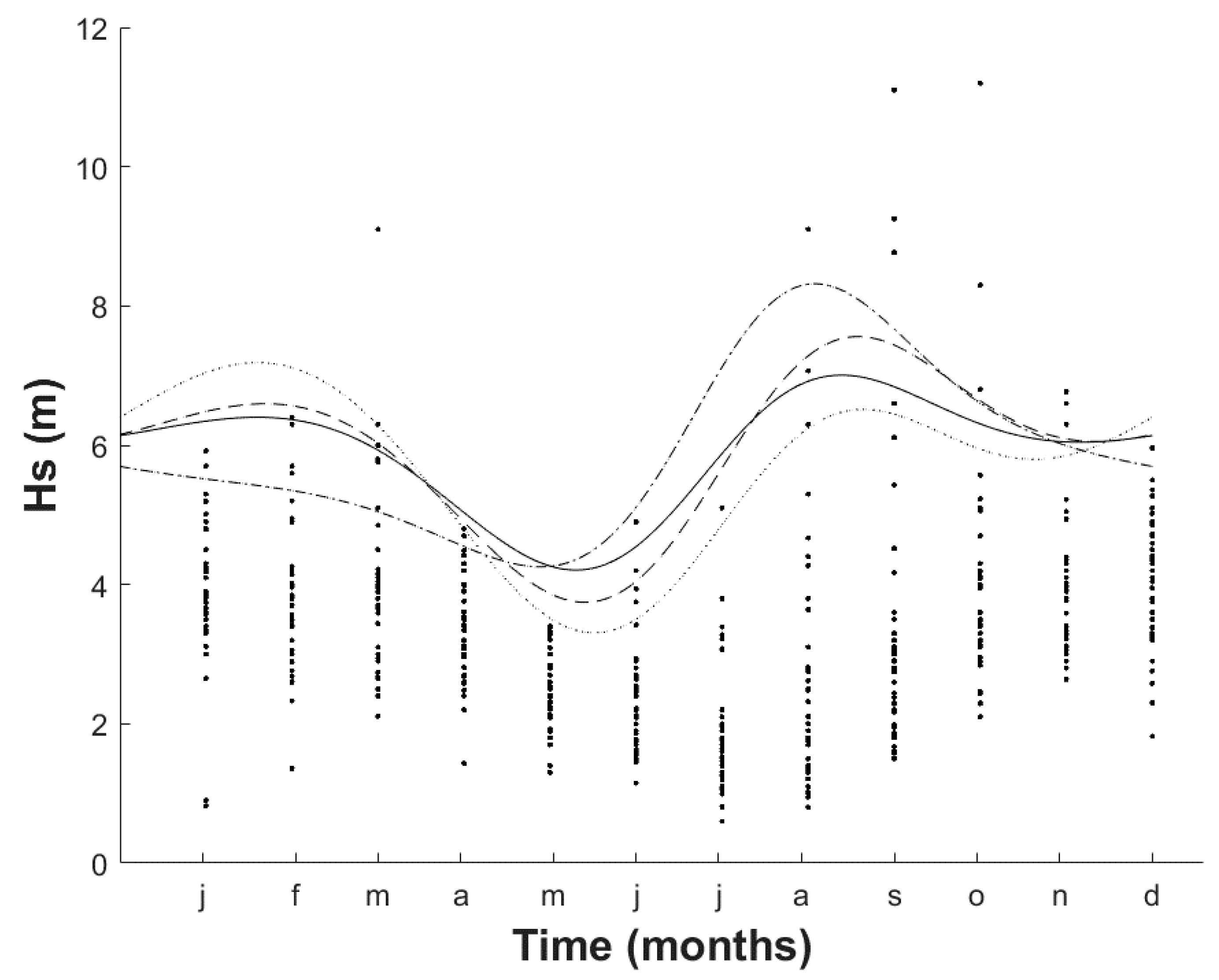
Figure 1. Monthly maximum and 30-yr return period values of Hs using different time ranges.
Applsci 10 04794 g001
Figure 2. Monthly companion and 30-yr return period values of Vw using different time ranges.
Applsci 10 04794 g002
Figure 3. Regression and residual analysis by using (a) nonlinear (Equation (9)) and (b) linear (Equation (7)) models for October. Residuals using (c) Equation (9) and (d) Equation (7).
Applsci 10 04794 g003
Figure 4. Normal probability papers for residuals. October: (a) nonlinear model and (b) linear model. February: (c) nonlinear model and (d) linear model.
Applsci 10 04794 g004
Figure 5. Regression and residual analysis by using (a) nonlinear (Equation (9)) and (b) linear (Equation (7)) models for February. Residuals using (c) Equation (9) and (d) Equation (7).
Applsci 10 04794 g005
Figure 6. Comparison of exact and approximated (Equations (11) and (12)) 95% confidence intervals, considering October (upper row; (a) and (b) for non-linear and linear cases, respectively) and February (lower row; (c) and (d) for non-linear and linear cases, respectively).
Applsci 10 04794 g006
Figure 7. Regression lines and confidence intervals including (solid and dashed lines, respectively) and excluding (dashed–dotted and dotted lines, respectively) T-yr values for October; (a) and (b) for logarithmic space and linear space, respectively. Filled circles are given by T-yr values with embedded perpendicular lines indicating confidence intervals from GEV models.
Applsci 10 04794 g007
Figure 8. Residuals and normal probability papers including T-yr values in the regression: (a,c) for the logarithmic case and (b,d) for the linear case.
Applsci 10 04794 g008
Figure 9. Exact and approximated 95% confidence intervals for October considering the T-yr values: regression (a) in logarithmic space and (b) in linear space. Legends indicate expressions referred in [28].
Applsci 10 04794 g009
Figure 10. Regression lines and confidence intervals including (solid and dashed lines, respectively) and excluding (dashed–dotted and dotted lines, respectively) T-yr values for February; (a) and (b) for logarithmic space and linear space, respectively. Filled circles represent T-yr values with embedded perpendicular lines indicating confidence intervals from GEV models.
Applsci 10 04794 g010
Figure 11. Regression lines and confidence intervals including (solid and dashed lines, respectively) and excluding (dashed–dotted and dotted lines, respectively) T-yr values for August; (a) and (b) for logarithmic space and linear space, respectively. Filled circles represent T-yr values with embedded perpendicular lines indicating confidence intervals from GEV models.
Applsci 10 04794 g011
Figure 12. Exact and approximated 95% confidence intervals for February considering the T-yr values: regression (a) in logarithmic space and (b) in in linear space. Legends indicate expressions referred in [28].
Applsci 10 04794 g012
Figure 13. Exact and approximated 95% confidence intervals for August considering the T-yr values: regression (a) in logarithmic space and (b) in in linear space. Legends indicate expressions referred in [28].
Applsci 10 04794 g013
Table 1. Fitted parameters of regression analysis for buoy 42,001 in this study considering seasonality.
MonthFor Equations (8) and (12)For Equations (10) and (11)
1bασeεV(%)bασeεV(%)
January6.31300.50500.132312.66.02661.65651.83809.4
February4.63110.73320.14480.484.45972.08911.77350.73
March6.22700.52230.16926.926.55851.57312.05925.87
April4.72800.71170.17570.163.9142.18981.79270.44
May4.69220.66160.40189.55.06701.58912.723413.1
June6.36110.41040.320516.15.26391.72902.56234.2
July6.01590.51320.40055.74.30022.32812.947418.5
August5.52290.56480.35298.73.89722.17682.60759.3
September4.62090.75960.22955.42.74022.62592.60711.2
October5.12430.68230.16264.73.89332.34762.09730.03
November10.32530.10500.174234.010.58710.37361.972631.7
December4.66880.68600.189910.13.37222.21092.27035.5
1b = exp(β), where β is the intercept obtained from the regression in the logarithmic space.