Ocular Biometrics Recognition by Analyzing Human Exploration during Video Observations

Abstract

Soft biometrics provide information about the individual but without the distinctiveness and permanence able to discriminate between any two individuals. Since the gaze represents one of the most investigated human traits, works evaluating the feasibility of considering it as a possible additional soft biometric trait have been recently appeared in the literature. Unfortunately, there is a lack of systematic studies on clinically approved stimuli to provide evidence of the correlation between exploratory paths and individual identities in “natural” scenarios (without calibration, imposed constraints, wearable tools). To overcome these drawbacks, this paper analyzes gaze patterns by using a computer vision based pipeline in order to prove the correlation between visual exploration and user identity. This correlation is robustly computed in a free exploration scenario, not biased by wearable devices nor constrained to a prior personalized calibration. Provided stimuli have been designed by clinical experts and then they allow better analysis of human exploration behaviors. In addition, the paper introduces a novel public dataset that provides, for the first time, images framing the faces of the involved subjects instead of only their gaze tracks.

1. Introduction

Biometrics encompasses the science of measuring individual body characteristics in order to distinguish a person among many others (hard biometrics). The first idea of identifying people based on biometrics dates back at the end of the 19th century with the seminal works in [1,2]. Those works encompass the application of a scientific approach based on different traits that are nowadays classified and recognized as soft biometrics: in facts, the considered traits were the color of the eyes, shape and, size of the head, height, weight, scars, and tattoos. Soft biometrics are defined indeed in terms of characteristics that provide information about the individual but without the distinctiveness and permanence able to discriminate between any two individuals [3]. They can be categorized as physical, behavioral, or adhered human characteristics corresponding to pre-defined human compliant categories [4]. Compared with hard biometrics, these traits present stronger invariance [5] and they can be often extracted without requiring subject cooperation and from low-quality data [6]. Moreover, they can complement and strengthen hard primary biometric identifiers, since are established and time-proven by humans in order to differentiate their peers; as a consequence, one of the most successful and investigated solution is to strengthen classic biometric identification schemes [7,8,9]. Refer to [10] for a complete review. All of the aforementioned reasons make soft biometrics very appealing, as shown by the numerous works present in the literature, spacing from authentication [11] to customized robot behavior [12], from social networks users analysis [13] to healthcare [14].

On the other hand, the gaze represents one of the most investigated human traits since it expresses human emotions, feelings, and intentions. Recently, the possibility to consider gaze as a possible additional soft biometric trait has obtained a lot of attention from the scientific community. It is well known that there is a close relationship between what the eyes are gazing at and what the mind is engaged with, and this idea was formulated by Just and Carpenter in the “Eye-Mind Hypothesis” [15].

This evidence has been recently proved by using eye-tracker technology [16]. Unfortunately, such systems are usually expensive and invasive (in case of setup based on wearable helmet or glasses). Moreover, they work under constraints like head movement and/or distance from the target, often requiring the user cooperation during a time-consuming calibration procedure. The above drawbacks project a bias in the acquired data since behavioral patterns become not natural, but in some way adapted to respect the imposed constraints [17].

Exploratory studies under unconstrained scenarios have been recently carried out in [18,19,20], but they used either static images or few and very generic videos as stimuli, making difficult to draw settled conclusions. The motivations of this work can be then found in the lacks of systematic studies on clinically approved stimuli to provide evidence of the correlation between exploratory paths and individual identities in natural scenarios (without calibration, imposed constraints, wearable tools).

In this work, evidence of the natural correlation between the user’s scene exploration and soft biometric identification is provided. This is achieved by acquisition sessions in which different users watch visual stimuli on a screen. A consumer camera, pointing towards the user, is employed and the acquisition outcomes are given as input to an innovative computer vision pipeline that extracts the user gaze. The system does not require user calibration nor impose constraints in terms of appearance, hairstyle, beard, eyeglasses, etc. The camera has been integrated into the scene in an ecological setting. Individuals were informed that a camera would record them but did not know the purpose of scientific research to minimize bias on visual exploration behaviors. Subsequently, gaze data are fed to a classifier that estimate the identity among a set of users.

Experiments have been performed on image sequences of two datasets. In particular, one of them has been introduced in this paper and it represents, to the best of our knowledge, the first dataset specifically designed for analyzing facial cues during visual exploration. Differently from available datasets in the state of the art which contain gaze tracks extracted by an eye tracker, it contains also facial images of the different subjects and their information in terms of soft biometrics traits. Experimental results show the strong correlation among a user and his extracted gaze tracks, demonstrating how the gaze can be effectively used as soft biometrics also in natural contexts.

Summing up, the main contributions of this paper are:

• it analyzes gaze patterns by using a computer vision-based pipeline to prove the correlation between visual exploration and user identity. This correlation is robustly computed in a free exploration scenario, not biased by wearable device and constrained to a prior personalized calibration;
• it introduces a novel public dataset that can be used as a benchmark to improve knowledge about this challenging research topic. It is the first dataset that directly provides images framing the faces of the involved subjects instead of their gaze tracks extracted by an eye tracker (unlike all the available datasets aimed at improving biometric analysis of gaze patterns).

The remainder of the manuscript is organized as follows: in Section 2 the related work is introduced, while the method is exposed in detail in Section 3. Section 4 reports the description of the two datasets employed during the experiments, introduced and evaluated in Section 5. Section 6 concludes the manuscript.

2. Related Work

It is known that eye movements are correlated to the scene, but the exploration also depends on the specific task the user is performing [21], and this relation has been massively investigated [22]. However, some properties of the scene, like the presence of regions with a high feature density [23] and/or moving parts [24], have a direct impact on the visual exploration patterns. The study of such properties has lead to a plethora of works investigating the intrinsic properties of the scene [25,26], with applications in human behavior prediction [27], scene segmentation [28], gaming [29], and human–computer interaction [30]. In fact, similarities between the fixation patterns of different individuals have been employed to predict where and in which order people look [31].

Nevertheless, since the last two decades, also the uniqueness of visual exploration and the possibility to design personalized gaze profiles for a scene have been investigated [32,33]. In the work of [34], personalized profiles have been created from eye-tracking data while users were watching at a set of images, showing that the system can differentiate among 12 users with accuracy ranging between 53% and 76%. In [35], user-dependent scans have been employed to evaluate parameters like observation time and spatial distribution while looking at different human faces. These scans have been employed to distinguish between different genders and age groups (in particular between persons under/over 30 years old). The same technique has been employed to distinguish between individuals among a group in [36]. Authentication by using dynamic saccadic features to generate a model of eye movement-driven biometrics has been also provided on a larger database of users in [37]. In [38], an authentication system that exploits the fact that some eye movements can be reflexively and predictably triggered has been proposed, without requiring any user memorization nor cognitive effort.

An attempt to standardize the research on the theme has been given by the “Eye Movements’ Verification and Identification Competition (EMVIC)” in 2012 [39], providing different datasets and giving a common performance benchmark for the task of user identification among a set. The classification results gave big evidence of the feasibility of considering the gaze as biometrics. A complete survey on the related work on visual exploration as biometrics can be found in [40].

Very few works in the state of the art tried to achieve soft biometrics identification by using a consumer camera pointed towards the user. A very early work trying to distinguish individuals on the way of looking has been proposed in [18]. The system used static images as stimuli, and it estimated the gaze on a technique based on visual salience [41]. Two seminal works that showed how the temporal evolution of gaze tracks acquired by an uncalibrated and non-invasive system can be used as soft biometrics are in [19,20]. Both works employed a depth sensor, requiring a precise depth map to estimate the user gaze. Moreover, here stimuli are represented by videos extracted from YouTube, not specifically designed for the purposes under consideration. Recently, mouse movements have been merged with eye tracking data coming from commercial software (i.e., “The Eye Tribe”) to improve soft biometrics classification [42]. Nevertheless, identification is performed on users clicking at a set of circles on the screen to enter a PIN number. To the best of our knowledge, the first and a unique attempt to provide soft biometrics identification by applying a computer vision pipeline to images coming from a consumer camera pointing at a user watching a video has been proposed in a preliminary study in [43]. Anyway, authors exploited stimuli videos extracted from a dataset suitable to evaluate the performance of gaze estimation algorithms.

Recently, the vasculature of the sclera (unique for each individual) has been considered for biometric recognition systems [44]. The study has been carried out proposing a new dataset, but it represents a vascular biometrics modality and does not consider visual exploration patterns.

3. Proposed Method

A block diagram of the proposed solution is reported in Figure 1. Input is given by a video of a user watching a scene on a computer screen (refer to Section 4 for more details on the visual inputs given to the user). For each image, the presence of the face in the scene is detected, and the user gaze vector is estimated in terms of its 3D components. The gaze information, for each iteration and of each video observed by each user, is opportunely aggregated in matrix form, and sparse principal component analysis (SPCA) is performed to extract dominant features. Such features are employed by a downstream classifier that estimates the final identity of the observer. In the following, each block is detailed.

3.1. Face Detection

First of all, the face is detected by means of the reduced ResNet-10 Single Shot MultiBox Detector (SSD) [45]. This solution drastically reduces the number of misdetections and false detections (to such an extent that no false positives and false negative occurred during the experimental phase).

3.2. Gaze Vector Estimation

The region of the image containing the face is the input for the Gaze Vector Estimation block. First of all, 68 2D facial landmarks are detected and tracked on the face region employing a probabilistic patch expert named Conditional Local Neural Fields (CLNF). This way, spatial and non-linear relationships between pixels (neighboring and longer distance) and the alignment probability of a landmark [46] are learned. The employed patch expert is the Local Neural Field (LNF), an undirected graph that models the conditional probability of the probability that a patch is aligned ($\mathbf{y}$) depending on the pixel intensity values in the support region. It also includes a neural network layer that can capture complex non-linear relationships between pixel values and the output responses.

For a particular set of observations of pixel intensities $\mathbf{X}=\{x_1,x_2,\dots ,x_n\}$, the set of output variables $\mathbf{y}=\{y_1,y_2,\dots ,y_n\}$ is predicted by the model that is the conditional probability distribution with density:

$$P\left(\mathbf{y}\right|\mathbf{X})=\frac{exp\left(\psi \right)}{{\int }_{-\infty }^{\infty }exp\left(\psi \right)dy}$$

(1)

The potential function $\psi$ is defined and determined by four model parameters $\{\alpha ,\beta ,\gamma ,\mathsf{\Theta }\}$ that are learned by maximizing the conditional log-likelihood of the LNF on the training sequences. See [46] for more details.

The locations of facial feature points in the image are modeled using non-rigid shape and rigid global transformation parameters trained on the LFPW [47] and Helen [48] datasets. The CLNF is further optimized with a Non-uniform Regularized Landmark Mean-Shift technique [49]. Once the 2D-3D correspondences are known, the 3D rotation and translation vectors $R,T$ are found by the Perspective-n-Point algorithm based on Levenberg–Marquardt optimization [50] to map the detected 2D landmark position and a static 3D head pose model.

In particular, given the camera intrinsic calibration matrix K as:

$$K=\left[\begin{array}{ccc}{f}_x& 0& c_x\\ 0& f_y& c_y\\ 0& 0& 1\end{array}\right],$$

(2)

then, for each correspondence between a landmark in image plane coordinates ($p_{IP}$) and 3D point (subscript $p_{3D}$) we have:

$$s{p}_{IP}=K\left[R\right|T]p_{3D}$$

(3)

whose least-squares solution represents the 6-DOF pose of the face.

The information provided by the generic CLNF deformable shape registration is applied to the eye region to find the location of the eye and the pupil and, consequently, to compute the eye gaze vector for each eye as suggested in [51]. For this step, training of the CLNF model is performed on the SynthesEyes [52], a dataset of eye-patches synthetically generated. Gaze vector is computed in the following way: a ray is cast from the camera origin through the center of the 2D pupil pixel position, and its intersection with the eyeball sphere is used to estimate 3D pupil position. The vector passing from the two 3D points represented by the eyeball and the pupil is the estimated gaze vector. In the proposed pipeline, the gaze vector is estimated only for the right eye, extracting its $x,y,z$ coordinates.

3.3. Data Aggregation and FIR Smoothing

Gaze data representing one user watching one video is stored. We denote with:

• $i\in [1\dots N_{subjects}]$ the subject i, where $N_{subjects}$ is the total number of participants;
• $j\in [1...N_{videos}]$ the j-th video, where $N_{videos}$ is the total number of different videos;
• $k\in [1...N_{session}]$ the k-th session, where $N_{session}$ is the total number of session performed by the subjects.

First of all, for each $i,j,k$, the extracted N gaze tracks are concatenated in one vector $S(i,j,k)$ in the following way:

$$S(i,j,k)=\left[x\right(1),\dots ,x(N),y(1),\dots ,y(N),z(1),\dots ,z(N\left)\right]$$

(4)

If the gaze in a frame n is not detected, then the triplet $\left(x\right(n),y(n),z(n\left)\right)$ takes values $(0,0,0)$. Since videos have different lengths, zero padding is used in all videos (except the longest one) to force all the vectors having the same length. The vector $S(i,j,k)$ is created for each video, subject and (eventually) session, obtaining a sparse matrix D of size $(N_{subjects}·N_{videos}·N_{session})\times 3N$. In the case of input data not divided in different sessions (see Section 4), then simply $N_{session}=1$. The last part of this processing step aims at filtering data using a Savitzky–Golay Finite Impulse Response (FIR) filter to perform smoothing [53]. In particular, as detailed by Schafer in [54], a polynomial function of the N-th degree, $p\left(n\right)$, is fit on the data by minimizing the sum of squared residual with the original sequence of samples, $x\left[n\right]$, on a window of size $2M+1$. Therefore, a set of $N+1$ polynomial coefficients $a_k$ is found for every sample in x using Equations (5). The idea behind this process is to perform least-squares polynomial smoothing to $p\left(n\right)$ with a set of coefficients that minimize the mean-square approximation error ${ϵ}_n$, defined as in Equation (6), for the group of input samples centered at $n=0$.

$$p\left(n\right)=\sum _{k=0}^N{a}_k{n}^k$$

(5)

$${ϵ}_n=\sum _{n=-M}^M{(p\left(n\right)-x\left[n\right])}^2=\sum _{n=-M}^M{(\sum _{k=0}^N{a}_k{n}^k-x\left[n\right])}^2$$

(6)

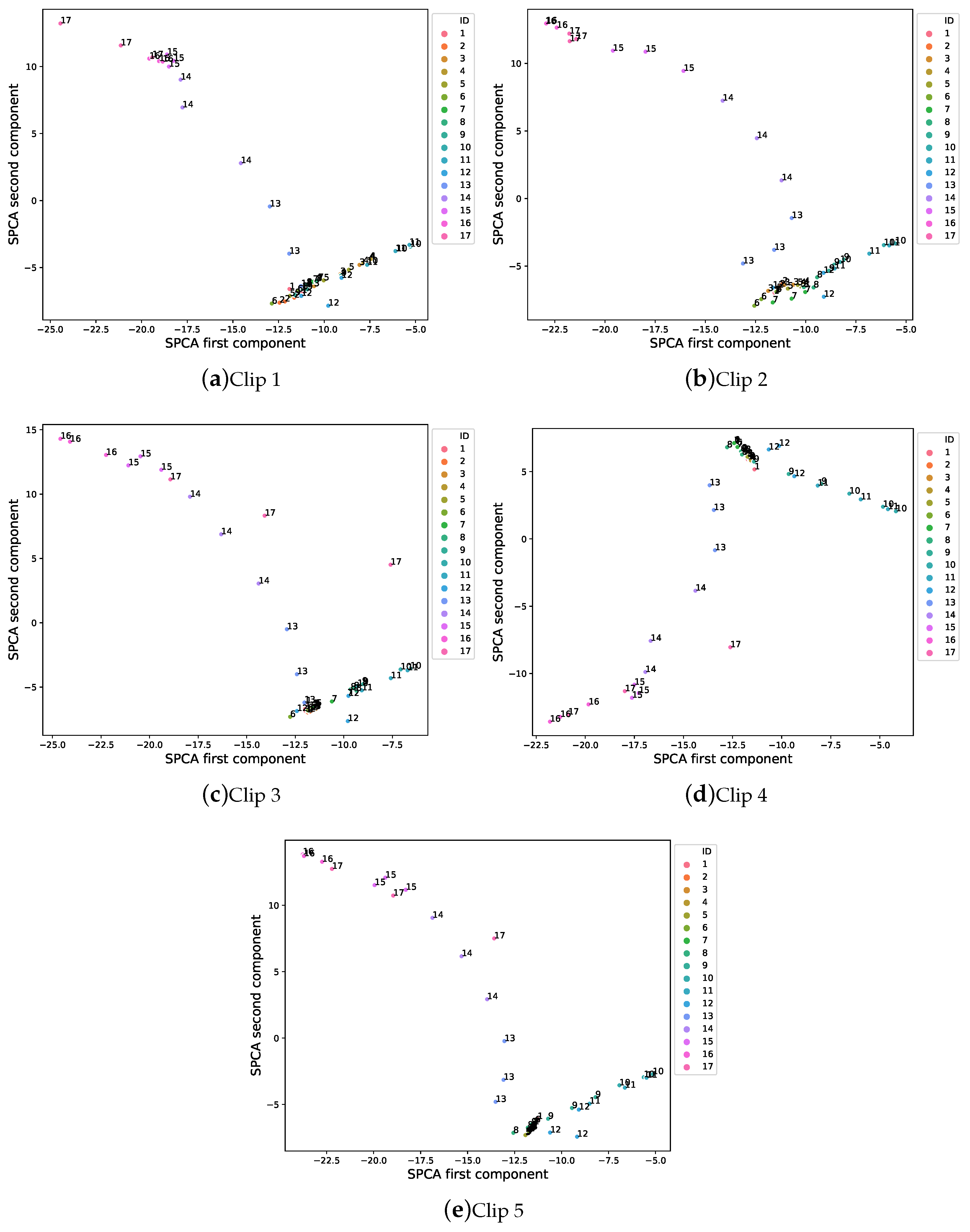
3.4. Sparse Principal Component Analysis

In the practice, the matrix obtained using the previous processing blocks is sparse, due to frames where people did not look at the screen or in general because the pipeline was not always able to extract gaze data. In order to extract the most informative features for the matrix under consideration, we used the sparse principal component analysis using the inverse power method for nonlinear eigenproblems (NIPM) implementation [55]. Given a symmetric matrix A, it is possible to characterize its eigenvectors as the critical point of the functional $F\left(f\right)$ s.t.:

$$F\left(f\right)=\frac{<f,Af>}{{\left|\right|f\left|\right|}_2^2}$$

(7)

It is possible to compute eigenvectors of A with the Courant–Fischer Min-Max principle. In this work we consider functionals F of the form $F\left(f\right)=R\left(f\right)/S\left(f\right)$ with $R,S$ convex, Lipschitz continuous, even, and positively p-homogeneous for $p\ge 1$. In the proposed pipeline, the number of retained components C of the SPCA is always set such that the 95% of the variance is always retained (variance-based a priori criterion) [56].

3.5. k-Nearest Neighbors

The identity of a person is assessed by a k-nearest neighbors (k-NN) classifier [57] based on the Euclidean distance between the elements of the matrix rows $\tilde{S}(i,j,k)=(s_1,s_2,\dots ,s_C)$ (the ∼ symbol over the letter S is added to represent the feature vector $S(i,j,k)$ after the SPCA). The parameter k represents the number of nearest neighbors to consider in the majority of the voting process and it is the only parameter that must be given a priori to the pipeline in order to make an identity estimation.

4. Dataset

In this work, two different sets of data have been used to give evidence of the possibility to use the proposed algorithmic pipeline to associate visual exploratory patterns to biometric information. The first dataset is the publicly available TabletGaze introduced in [58]. The dataset consists of videos recorded by the front camera of a tablet, while 51 subjects, 12 females and 39 males, watched the stimuli (clips) projected on the screen of the device itself held in their hands. The clips watched by the subjects consist of a dot changing its location every 3 s, and the subject was instructed to focus his/her eyes on the dot the whole time. Different videos were acquired by the same subject in this unconstrained mobile setting. In this paper, 4 videos per subject are used, i.e., the 4 videos in which the subjects were in standing position which are the only ones fully containing the face. Videos of 22 of 51 subjects (having ids 1’, ’2’, ’3’, ’4’, ’5’, ’6’, ’9’, ’11’, ’12’, ’15’, ’17’, ’19’, ’23’, ’27’, ’29’, ’37’, ’39’, ’40’, ’44’, ’49’, ’50’, ’51’) were taken into consideration. This subset was chosen considering only subjects who maintained at least half face visible for most of the time. Thus, a total of 88 videos were processed.

The second dataset was instead expressly acquired for the purposes of this paper. In particular, 17 different subjects (12 men, 5 women) aged in the range of 4-46 years were involved. In particular, there was a kid of preschool age (4 years old) and a school-age kid (9 years old), whereas the remaining subjects were all adults. Each subject was asked to position himself in front of a 27-inch monitor at an approximate distance of about 70 cm, and a webcam recorded his face while 5 short clips of about 20 s each were projected on the screen.

The seventeen introduced subjects have been recorded while watching each clip during three different sessions. Each session has been performed with at least 24 h interval. Associated gaze information, extracted by using the pipeline in Section 3, are reported. In addition, other soft biometrics traits regarding the age and gender of the participants have been inserted in the dataset. The dataset consists of video files of the recorded sessions and a command separated values (CSV) structure where each line contains information like age, gender, identity, and temporal gaze tracks of the participant. Figure 2 reports one frame of the dataset extracted by seven participants.

Stimuli were selected among those collected in [59]. In particular, the five visual stimuli summed up in Figure 3 were selected. The figure shows their filename as in the original dataset (Available at: http://www.inb.uni-luebeck.de/tools-demos/gaze). All stimuli consist of high-resolution movies of real-world scenes recorded by a JVC JY-HD10 HDTV video camera. The audio was set off. All clips have a length of about 20 s; their temporal resolution was 29.97 frames per second and their spatial resolution was $1280\times 720$ pixels (NTSC HDTV progressive scan). All clips were stored to disk in the MPEG-2 video format with a bit rate of 18.3 Mbit/s. The camera was fixed on a tripod. The first three clips contained no camera or zooming movements whereas the sequences depicting animals (bumblebee and doves) contained minor pan and tilt camera motion. The choice of the stimuli was based on the theory that a very low variability, for example using a scene on which all observers follow the same gaze pattern, offers little room to guide the observer’s attention; at the same time, a very high variability might indicate the dominance of idiosyncratic viewing strategies that would also be hard to influence. In other words, the selected stimuli have a variability level that is ideal to drive the viewer to follow personalized visual patterns depending on the objects that the user finds most important (without boredom, in case of scene stillness, or idiosyncrasy, in case of too complex and variable stimuli) [60].

In particular, Clip 1 frames a beach area in which a high number of people are performing activities like running, playing or simply standing while talking to each other. People can appear everywhere in the scene so it becomes necessary to focus on a part of it in order to understand what it is happening. Clip 2 shows an urban scenario: there is a pedestrian street in which many people pass longitudinally with regards to the field of view of the camera. Clip 3 frames a lake with a bridge in the background and a small house behind the bridge. All around there is vegetation. The wind moves the water and vegetation, but nothing happens during the entire duration of the video. Clip 4 begins by framing a small portion of land with dense vegetation. At a certain point, a bumblebee appears from behind the leaves and at a certain point it takes off while the camera follows its movement. Finally, in Clip 5, there is a square with some pedestrians and some doves who are pecking for bread crumbs. The shot focuses and follows the doves.

Several studies have been conducted to determine the contribution of different features to the deployment of attention. The most relevant study in this area introduced the concept that visual attention is guided by several attributes [61]. According to the above theory, the video to be used as stimuli were selected in order to include the most relevant guiding attributes. In particular, the included attributes are the following: fast motion (Clip 2), dynamic background (Clip 1), occlusion (Clip 4), search for most dynamic elements in static scenes (Clip 3), and multiple foreground objects (Clip 5), also considering both static (Clip 1, Clip 2, Clip 3) and moving cameras (Clip 4, Clip 5). Figure 3 reports a frame of each clip used as stimuli in the Experimental Phase #2 (see Section 5.2).

Videos of the 17 subjects involved in this experimental phase were recorded using an oCam-5CRO-U, a 5 megapixels high-resolution color camera. Videos were acquired at 28.86 fps with a $1280\times 720$ spatial resolution. All videos were stored to disk in the MPEG-4 video format with a bit rate of 7.9 Mbit/s.

Together with the user videos, the datasets consists of a Comma-Separated Values (CSV) file with the following information:

• Column 1: name of the file video;
• Column 2: age of the participant;
• Column 3: gender of the participant (M/F);
• Column 4: user ID;
• Column 5: session number;
• Column 6: clip number;
• Column 7-END: vector $S(i,j,k)$ (composed as described in Section 3.3).

The dataset is publicly available at https://dataset.isasi.cnr.it/.

It is useful to remark again that, while acquiring videos, no restrictions were given to the subjects about eye blinking, head position, geometry with regards to the acquisition sensor. The presence of the camera for acquiring the involved individuals represents the only “external” element in a completely natural scenario. However, as already stated in the introductory section, the camera has been integrated into the scene in an ecological setting. Involved individuals were informed that a camera would record them but did not know the purpose of scientific research to minimize bias on visual exploration behaviors. As a general consideration, it is worth noting that for ethical reasons it is not possible to acquire individuals without making them aware of the camera. All research with human participants requires formal and informal adherence to procedures that protect the rights of the research participants. However, scientific pieces of evidence demonstrated that the presence of a camera mainly alters pro-social and cheating behaviors [62] whereas, under settings similar to the experimental one, the human behaviors keep unaffected by the awareness of the recording procedure [63].

5. Experiments and Results

Since works in the state of the art (refer to Section 2) that proposed gaze as soft biometrics employed a professional eye tracker, the first experimental phase aims at evaluating the capability of the proposed pipeline to get gaze information suitable for the task under consideration. In this regard, image sequences available in the TabletGaze have been employed. Anyway, the TabletGaze dataset consists of videos of a dot changing its location every few seconds. Subsequently, in order to provide evidence of biometrics identification depending on the subject’s visual exploration of natural scenes, a second experimental phase has been carried. The two different experimental phases, as well as their results, have been detailed in the following.

In both experimental phases, the employed FIR smoothing filter is of polynomial order 3 and frame length 11. The facial model and software described in Section 3 have been employed. The code has been developed using Python. The parametrization of the Support Vector Machine during training has been fixed with a value of $C=10$ and with gamma set to $1/d$, where d is the feature vector dimensionality. For k-NN, the value of k has been set to 1 for all the experiments due to the low number of samples per each class. All the features have been normalized before the training phase by removing the mean and diving by the standard deviation.

5.1. Experimental Phase #1: System Validation

The 22 videos introduced in Section 4 were processed during the first experimental phase. In each video, the algorithmic pipeline described in Section 3 was applied without any prior knowledge about initial calibration nor environmental settings/body posture. Considering the length of the longest video ($n=18,103$), data is gathered in a matrix D of dimensions $88\times 54,309$. Since each subject watched each video only once in this experimental phase, we have:

• $N_{subjects}=22$
• $N_{videos}=4$
• $N_{session}=1$

SPCA is applied to the matrix and the first 20 components, roughly corresponding to the $95\%$ of the data variance, are retained. In Figure 4a, two dimensional t-Distributed Stochastic Neighbor Embedding (t-SNE) [64] of the SPCA projected data is plotted for visualization purposes. This technique creates an embedding so that similar objects, with a probabilistic interpretation of similarity, are modeled by nearby points and dissimilar objects are modeled by distant points. Hence, nearby points in the higher dimensional space have more probability to be represented together, while points with larger Euclidean distance are pushed even more apart in the embedding due to the heavy tail of the t-Student distribution. Perplexity parameter loosely determines how to balance attention between local and global aspects of data, representing a guess about the number of close neighbors each point has. As can be observed from the figure, it becomes evident how subjects form clusters in the embedding space. This preliminary result gives us qualitative evidence that the system is able to distinguish the way a person is looking at the screen, giving also evidence of the relationship between single gaze tracks and subject identity.

In order to provide quantitative evidence of the proposed pipeline to identify subjects, an analysis of distance ranks has been performed [43]. For each feature vector, the Euclidean distance among other vectors is computed, varying the number of used principal components. We associate rank for the instance n of the subject m as:

$$rank(m,n)=l$$

(8)

where l is the lowest position in the ordered (in ascending order) array of all mutual distances. For example, if the subject m at the instance n has its closest vector in correspondence of another of his remaining 3 videos, then $rank(m,n)=1$, while it will be 2 if the distance with one of the remaining 3 videos is represented by the second element of the ordered array, and so on. The rank calculated for $m\in [1,22]$ and $n\in [1,4]$ as well as varying different retained components in the feature vector of the SPCA is reported in Figure 5.

The x-axis reports the number of retained components, while the y-axis shows the number of occurrences of $rank=1$. It can be observed how the maximum number of occurrences of $rank=1$ is achieved in correspondence of 30 components. Instead, the proposed automatic variance-based criterion of Section 3 gives us the value of 20 components. This misalignment is motivated by an absence of direct correspondence between the SPCA and our introduced definition of rank. Anyway, we expect that a “best practice”, like the heuristic criterion of retaining the 95% of the variance, can provide a good insight of the data. Moreover, it would be unfair to set a static number of components after the analysis of classification outcomes. To that end, a comparison of rank values after having fixed one of these two values is reported in Figure 6. To the left (Figure 6a) it is reported the case of using the variance as a dynamic criterion to establish the number of components to retain, while the plot of the rank values with a posteriori criterion is reported in Figure 6b. First of all, it is worth to note that rank is always 1 or 2, except for one case, and this represents an impressive result. Moreover, in both cases the rank shows a similar behavior, with only one occurrence of $rank=3$ for the a posteriori case, giving experimental evidence of the validity of a dynamic approach.

Finally, a simple assessment of the last block composing the proposed system has also been performed with the dataset under consideration. The proposed k-NN is compared with the SVM performance varying the number of SPCA components introduced on the same dataset of [43]. Results are plotted in Figure 7, where each value of accuracy is the average of the classification results validated using a leave-one-out procedure. As it can be observed, the k-NN outperforms the SVM classifier.

5.2. Experimental Phase #2: Soft-Biometrics Identification

In the case of the UserWGaze dataset, we have:

• $N_{subjects}=17$
• $N_{videos}=5$
• $N_{session}=3$

Anyway, considering the different nature of videos, the identification has been performed for every single video, making five separate analyses. Thus, each matrix will have the shape $(N_{subjects}·N_{session})\times M$, i.e., $51\times M$, with M being the number of frames of each video used in the test. Variances associated with the SPCA direction for the five clips used with experiments on the UserWGaze dataset are reported in Figure 8. It can be observed that for any video the criterion is respectively retaining nine components.

Figure 9 reports the subjects-related data distribution on the first and second components of the SPCA projected data for each of the five clips used as stimuli (see Section 4). From the figure, it is possible to derive some very useful considerations. Representation of components extracted while people watched at Clip 1 reveals that there are different agglomerations of points already in two dimensions. It is straightforward to derive that this comes from the contents of the video that contained a lot of objects and people moving in every part of the images. Each observer needed to explore the whole scene to be able to focus, in a sequential manner, on the different situations displayed over time. In addition, since the scene was acquired from a beach, people who have watched the scene were calm and they had a positive feeling and thus they performed a very slow exploration. This low arousal is likely the reason why, very surprisingly, the exploration was quite similar for some people (e.g., people 2-4-15) in the course of experimental sessions and this is evident from the proximity of many points belonging to the same individual. Other individuals explored the scene in a different manner in each session (e.g., people 10-13-14) and the related points appear a little bit far in the plot.

Data acquired while people watched Clip 2 seem to confirm this hypothesis: in this video, the moving objects are concentrated in the central part of the images and there is a more ordered sequence of events (pedestrians moving longitudinally with regards to the camera view). As a consequence, in collected data, it is possible to note a greater aggregation of points in a unique area of the plot (lower-right). Clip 3 further confirms the above consideration: it is a video without moving objects and this brought to a very compact representation of data with a very high aggregation of points belonging to the same people. It is evident that each person explored the scene in a different manner having no moving objects that drew his attention. At the end of the analysis of the first three videos (i.e., the clips with static camera), it is possible then to summarize that the larger the number of moving objects in the scene and their spreading in the images, the larger the scene exploration variability among people (interclass variance). On the other hand, also the likelihood that the same person looks at the scene in a different manner during different acquisition sessions depends on the aforementioned scene complexity (intraclass variance). In the case of a camera following a moving object, like in Clip 3 and Clip 4, the interclass variance becomes lower, but the intraclass variance decreases much more rapidly, making this way still possible to see very compact clusters in data points.

Obviously, this behavior is much more evident in the case of a single moving object (the bumblebee in Clip 4) than in the case of multiple objects (the doves in Clip 5).

The same t-SNE visualization has been reproduced for the five clips and results are shown in Figure 10. With this representation, the empirical evidence of the similarity of gaze features for the same subject during different sessions is even more evident, since all the retained dimensions are shrunk in the 2D view.

Classification performance has been assessed through a leave-one-out validation with the five videos of UserWGaze dataset.

A precise comparison with the pipeline proposed by [43] varying the number of retained components is reported in Figure 11. From the plots, it emerges that the highest accuracy is obtained at different numbers of retained components for each clip, but a drop in classification performance is common to the two cases under comparison. Therefore, although the choice of 95% variance components is sub-optimal for all the clips, the plots point out that using all the components markedly deteriorates the accuracy of the classifiers. Hence, the proposed heuristic provides a mean to prune those unnecessary biometrics features that would harm the user identification. However, we are aware that a better or optimal choice could be taken either individually for each clip or globally for the complete dataset. A direct comparison in terms of classification outcomes between the proposed variance criterion and taking all components is provided in

Table 1. Tables of the average accuracy for each of the five clips in the UserWGaze dataset. (a) The performances of SVM and k-NN are compared using the first 9 SPCA components, which represent about 95% of the variance; (b) the results of the case with 50 SPCA components and the total are given.

(a)
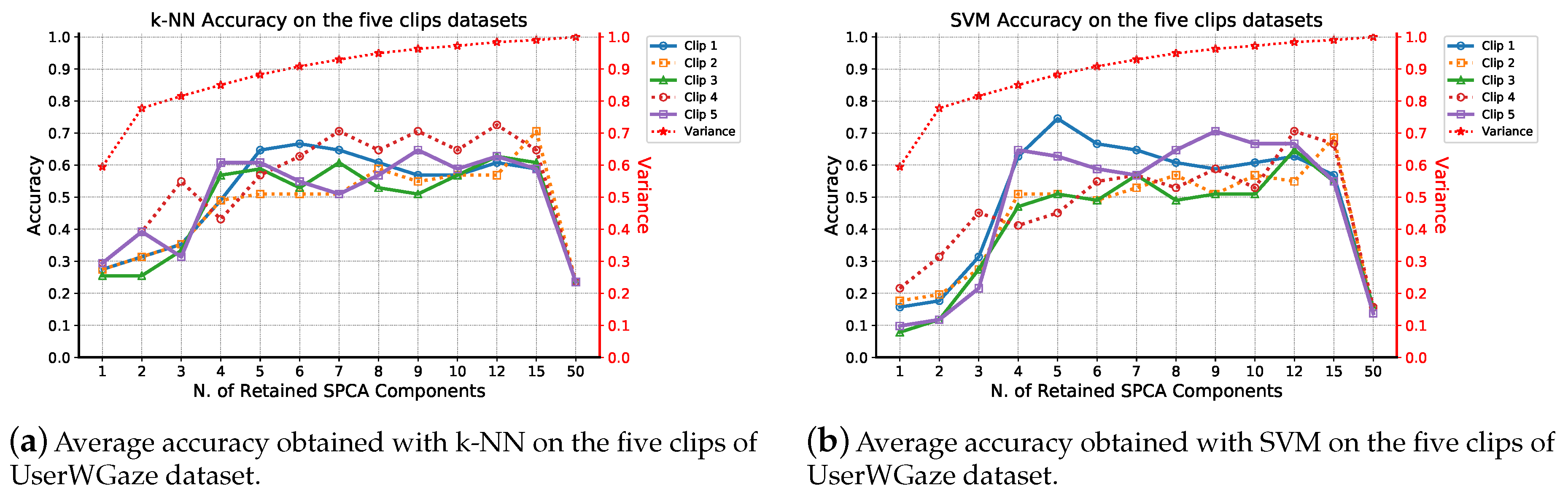
Clip #	N. of Components	SPCA Variance	SVM Accuracy	k-NN Accuracy
4	9	0.961	0.51	0.51
3	9	0.954	0.59	0.71
2	9	0.963	0.71	0.65
1	9	0.960	0.59	0.57
5	9	0.958	0.51	0.55
(b)
Clip #	N. of Components	SPCA Variance	SVM Accuracy	k-NN Accuracy
4	50	1.000	0.16	0.24
3	50	1.000	0.16	0.24
2	50	1.000	0.14	0.24
1	50	1.000	0.16	0.24
5	50	1.000	0.14	0.24

.

Inspired by the metrics proposed by Proenca et al. [65] to evaluate intra and interclass variation, the possibility to measure the stability (intraclass) and discriminability (interclass) while varying the number of retained SPCA components has been analyzed. In particular, the separability of the subject i-th has been defined as in Equation (9):

$$Stability\left(C_i\right)=1-\frac{1}{2t_i{t}_c}\sum _{x\in C_i}\sum _{y\in C_i}d{(x,y)}^2$$

(9)

where $t_i$ is the number of samples of the subject, $t_c$ the number of SPCA components, $C_i$ the centroid of the features vectors related to the i-th subject, d is the Euclidean distance function. Thus, the global stability is defined as the average of the $Stability\left(C_i\right)$, i.e., (Equation (10)):

$$Stability=\frac{1}{t_s}\sum _{i=1}^{t_s}Stability\left(C_i\right)$$

(10)

The discriminability, instead, is defined as in Equation (11):

$$Discriminability=\frac{1}{2K}\sum _{i=1}^K\sum _{j=1}^K\frac{t_i}{K}d{(c_i,c_j)}^2$$

(11)

where $c_i$ and $c_j$ are the average computed, respectively, on the points composing the clusters i and j, and K the number of subjects. Results are plotted in Figure 12. It is worth noting that stability monotonically increases while considering more components, whereas the discriminability value decreases while less than about 50 components are retained, before slightly increasing again. This suggests that the trade-off between stability and separability is to retain a number of components that are almost in the middle of the range [0–50].

Since strictly related works in the state of the art dealt with the task of identification as a whole (clips and sessions were not separated [20] or not available [43]), a similar operation has been performed in the UserWGaze dataset by joining all sequences and afford a fair comparison. Figure 13 reports the SPCA, t-SNE, and classification analysis on the whole dataset. In this case, 28 components are retained. In particular, the 2D representation of the first two principal components is in Figure 13a, the embedding obtained with the t-SNE using the proposed pipeline is in Figure 13b), and a comparison of SVM and k-NN classifiers is in Figure 13c).

It can be observed that, even if sometimes SVM is more accurate, in most of the cases the k-NN based approach outperforms the SVM classifier, included when 28 components are chosen. Since the analysis of soft biometrics discriminability is usually carried out using hit/penetration plots, in Figure 14 the top-N accuracy varying the number of classes for different values of k of the k-NN classifier is reported. To get this plot, different values of k have been tested in order to have continuous confidence outcomes instead of the discrete ones (0 or 1). The plot confirms, once again, that the gaze patterns provide useful information to discriminate soft biometrics.

A final comparison with some leading methods in the state of the art is resumed in

Table 2. Comparison with related approaches in the state of the art. AUC stands for Area Under Curve, subj. for subjects., req. for required. Results marked with * have been reproduced on the UserWGaze dataset.

Work	Method	Accuracy	Dataset	Notes
Deravi et al. (2011) [18]	backwards Feature Selection + SVM	0.92	own data	initialization and calibration req.
Cantoni et al. (2015) [36]	features graph	0.8179 (AUC)	GANT (16 subj.)	eye tracker req.
Cazzato et al. (2016) [20]	geometric model + minimax	0.810	own data (12 subj.)	RGBD sensor req.
Kasprowski et al. (2018) [42]	statistic features + SVM	0.928	proprietary data (24 subj.)	calibration req.
Cazzato et al. (2019) [43]	CNN+SVM	0.937*	UserWGaze	a posteriori choice with rank analysis
Cazzato et al. (2019) [43]	CNN+SVM	0.851*	UserWGaze	a priori 95% variance criterion
Proposed method	CNN+k-NN (k=1)	0.886	UserWGaze	a priori 95% variance criterion

. In particular, five previous works have been compared and the most relevant performance and used benchmark dataset are reported for each of them. Some additional notes have been also added to highlight the pro and cons of each work. The table clearly shows that the accuracy in subject identification is comparable with that in the works [18,36,42] where, as depicted in the last column reporting notes, initialization, calibration, or expensive eye tracker are required. In addition, the proposed approach outperforms the work in [20], despite it removes the constraint of the previous work of using an RGBD sensor. The pipeline in [43] has been also compared and its results have been reproduced using the UserWGaze dataset. It can be observed that the maximum accuracy reached in [43] is higher but, in that work, authors used an a posteriori analysis, presenting a method that is not fully automated. In fact, authors employed the rank, but it needs the class label for a query vector. If the pipeline in [43] is reproduced applying the fully automatic approach, it is possible to observe how our solution is more accurate. Finally, two general considerations may be made: (1) it is here useful also to remark again that, differently from all the comparing approaches, in this paper, a new benchmark dataset is provided with both facial images and extracted gaze tracks, and (2) the proposed work describes the whole computer vision pipeline that works on raw images and provides evidence of the biometrics identification using extracted gaze tracks. Most of the previous works directly start from gaze tracks (mainly extracted by external tools or devices) instead. Alternatively, external interventions are required to assess the machine learning process.

6. Conclusions

In this work, a computer vision pipeline that gives computational evidence of the user’s gaze validity as a soft-biometrics even using a consumer camera has been presented. First of all, a gaze estimation algorithm has been employed to extract data during visual exploration scenarios. Subsequently, a proper user feature representation has been generated and used to distinguish among a set of users. A new UserWGaze dataset has also been introduced; it contains videos of different subjects watching a set of clinically approved stimuli during different sessions. Their soft-biometrics information, as well as the estimated gaze vector, have been made publicly available. Experiments have been carried out on the UserWGaze and the TabletGaze datasets; the results in terms of accuracy are very encouraging showing, as the best of our knowledge, the first possibility to use a consumer camera for the task under consideration. In future works, facial analysis in terms of other soft-biometrics (age, gender, facial expression) will be integrated in order to improve the recognition performance in the case of bigger groups of people.

References

- Bertillon, A.; Müller, G. Instructions for Taking Descriptions for the Identification Of Criminals and Others by the Means of Anthropometric Indications; Kessinger Publishing: Whitefish, MT, USA, 1889. [Google Scholar]
- Rhodes, H.T.F. Alphonse Bertillon, Father of Scientific Detection; Abelard-Schuman: London, UK, 1956. [Google Scholar]
- Jain, A.K.; Dass, S.C.; Nandakumar, K. Soft biometric traits for personal recognition systems. In Proceedings of the International Conference on Biometric Authentication, Hong Kong, China, 15–17 July 2004; Springer: Berlin/Heidelberg, Germany, 2004; pp. 731–738. [Google Scholar]
- Dantcheva, A.; Velardo, C.; D’angelo, A.; Dugelay, J.L. Bag of soft biometrics for person identification. Multimed. Tools Appl. 2011, 51, 739–777. [Google Scholar] [CrossRef]
- Jaha, E.S.; Nixon, M.S. Soft biometrics for subject identification using clothing attributes. In Proceedings of the IEEE International Joint Conference on Biometrics, Clearwater, FL, USA, 29 September–2 October 2014; pp. 1–6. [Google Scholar]
- Reid, D.A.; Samangooei, S.; Chen, C.; Nixon, M.S.; Ross, A. Soft biometrics for surveillance: An overview. In Handbook of Statistics; Elsevier: Amsterdam, The Netherlands, 2013; Volume 31, pp. 327–352. [Google Scholar]
- Abdelwhab, A.; Viriri, S. A Survey on Soft Biometrics for Human Identification. Mach. Learn. Biom. 2018, 37. [Google Scholar] [CrossRef]
- Zewail, R.; Elsafi, A.; Saeb, M.; Hamdy, N. Soft and hard biometrics fusion for improved identity verification. In Proceedings of the 2004 47th Midwest Symposium on Circuits and Systems, Hiroshima, Japan, 25–28 July 2004. [Google Scholar] [CrossRef]
- Jaha, E.S. Augmenting Gabor-based Face Recognition with Global Soft Biometrics. In Proceedings of the 2019 7th International Symposium on Digital Forensics and Security (ISDFS), Barcelos, Portugal, 10–12 June 2019; pp. 1–5. [Google Scholar]
- Dantcheva, A.; Elia, P.; Ross, A. What else does your biometric data reveal? A survey on soft biometrics. IEEE Trans. Inf. Forensics Secur. 2015, 11, 441–467. [Google Scholar] [CrossRef]
- Niinuma, K.; Park, U.; Jain, A.K. Soft biometric traits for continuous user authentication. IEEE Trans. Inf. Forensics Secur. 2010, 5, 771–780. [Google Scholar] [CrossRef]
- Carcagnì, P.; Cazzato, D.; Del Coco, M.; Distante, C.; Leo, M. Visual interaction including biometrics information for a socially assistive robotic platform. In Proceedings of the European Conference on Computer Vision, Zurich, Switzerland, 6–12 September 2014; pp. 391–406. [Google Scholar]
- Geng, L.; Zhang, K.; Wei, X.; Feng, X. Soft biometrics in online social networks: A case study on Twitter user gender recognition. In Proceedings of the 2017 IEEE Winter Applications of Computer Vision Workshops (WACVW), Santa Rosa, CA, USA, 24–31 March 2017; pp. 1–8. [Google Scholar]
- Leo, M.; Carcagnì, P.; Mazzeo, P.L.; Spagnolo, P.; Cazzato, D.; Distante, C. Analysis of Facial Information for Healthcare Applications: A Survey on Computer Vision-Based Approaches. Information 2020, 11, 128. [Google Scholar] [CrossRef]
- Just, M.A.; Carpenter, P.A. Eye fixations and cognitive processes. Cogn. Psychol. 1976, 8, 441–480. [Google Scholar] [CrossRef]
- Porta, M.; Barboni, A. Strengthening Security in Industrial Settings: A Study on Gaze-Based Biometrics through Free Observation of Static Images. In Proceedings of the 2019 24th IEEE International Conference on Emerging Technologies and Factory Automation (ETFA), Zaragoza, Spain, 10–13 September 2019; pp. 1273–1277. [Google Scholar]
- Matthews, O.; Davies, A.; Vigo, M.; Harper, S. Unobtrusive arousal detection on the web using pupillary response. Int. J. Hum. Comput. Stud. 2020, 136, 102361. [Google Scholar] [CrossRef]
- Deravi, F.; Guness, S.P. Gaze Trajectory as a Biometric Modality. In Proceedings of the International Conference on Bio-inspired Systems and Signal Processing (BIOSIGNALS-2011), Rome, Italy, 26–29 January 2011; pp. 335–341. [Google Scholar]
- Cazzato, D.; Leo, M.; Evangelista, A.; Distante, C. Soft Biometrics by Modeling Temporal Series of Gaze Cues Extracted in the Wild. In Proceedings of the International Conference on Advanced Concepts for Intelligent Vision Systems, Catania, Italy, 26–29 October 2015; Springer: Berlin/Heidelberg, Germany, 2015; pp. 391–402. [Google Scholar]
- Cazzato, D.; Evangelista, A.; Leo, M.; Carcagnì, P.; Distante, C. A low-cost and calibration-free gaze estimator for soft biometrics: An explorative study. Pattern Recognit. Lett. 2016, 82, 196–206. [Google Scholar] [CrossRef]
- Yarbus, A.L. Eye Movements and Vision; Springer: Berlin/Heidelberg, Germany, 2013. [Google Scholar]
- Zelinsky, G.J. A theory of eye movements during target acquisition. Psychol. Rev. 2008, 115, 787. [Google Scholar] [CrossRef] [PubMed]
- Tatler, B.W.; Baddeley, R.J.; Vincent, B.T. The long and the short of it: Spatial statistics at fixation vary with saccade amplitude and task. Vis. Res. 2006, 46, 1857–1862. [Google Scholar] [CrossRef]
- Itti, L.; Baldi, P.F. Bayesian surprise attracts human attention. In Advances in Neural Information Processing Systems; MIT: Cambridge, MA, USA, 2006; pp. 547–554. [Google Scholar]
- Borji, A.; Cheng, M.M.; Hou, Q.; Jiang, H.; Li, J. Salient object detection: A survey. Comput. Vis. Media 2015, 5, 117–150. [Google Scholar] [CrossRef]
- Yun, K.; Peng, Y.; Samaras, D.; Zelinsky, G.J.; Berg, T.L. Exploring the role of gaze behavior and object detection in scene understanding. Front. Psychol. 2013, 4, 917. [Google Scholar] [CrossRef] [PubMed]
- Judd, T.; Durand, F.; Torralba, A. A Benchmark of Computational Models of Saliency to Predict Human Fixations; MIT: Cambridge, MA, USA, 2012. [Google Scholar]
- Mehrani, P.; Veksler, O. Saliency Segmentation based on Learning and Graph Cut Refinement. In Proceedings of the British Machine Vision Conference, BMVC 2010, Aberystwyth, UK, 31 August–3 September 2010; pp. 1–12. [Google Scholar]
- Nelson, D. Using Gaze Detection to Change Timing and Behavior. US Patent No. 10,561,928, 18 February 2020. [Google Scholar]
- Katsini, C.; Opsis, H.; Abdrabou, Y.; Raptis, G.E.; Khamis, M.; Alt, F. The Role of Eye Gaze in Security and Privacy Applications: Survey and Future HCI Research Directions. In Proceedings of the 38th Annual ACM Conference on Human Factors in Computing Systems, Honolulu, HI, USA, 25–30 April 2020; ACM: New York, NY, USA, 2020; Volume 21. [Google Scholar]
- Cerf, M.; Harel, J.; Einhäuser, W.; Koch, C. Predicting human gaze using low-level saliency combined with face detection. In Advances in Neural Information Processing Systems; NIPS: San Diego, CA, USA, 2008; pp. 241–248. [Google Scholar]
- Maeder, A.J.; Fookes, C.B. A visual attention approach to personal identification. In Proceedings of the 8th Australian & New Zealand Intelligent Information Systems Conference; Queensland University of Technology: Brisbane, QC, Australia, 2003; pp. 55–60. [Google Scholar]
- Kasprowski, P.; Ober, J. Eye movements in biometrics. In Proceedings of the International Workshop on Biometric Authentication, Prague, Czech Republic, 15 May 2004; Springer: Berlin/Heidelberg, Germany, 2004; pp. 248–258. [Google Scholar]
- Yoon, H.J.; Carmichael, T.R.; Tourassi, G. Gaze as a biometric. In Medical Imaging 2014: Image Perception, Observer Performance, and Technology Assessment; International Society for Optics and Photonics: Bellingham, DC, USA, 2014; Volume 9037, p. 903707. [Google Scholar]
- Cantoni, V.; Porta, M.; Galdi, C.; Nappi, M.; Wechsler, H. Gender and age categorization using gaze analysis. In Proceedings of the 2014 Tenth International Conference on Signal-Image Technology and Internet-Based Systems, Marrakech, Morocco, 23–27 November 2014; pp. 574–579. [Google Scholar]
- Cantoni, V.; Galdi, C.; Nappi, M.; Porta, M.; Riccio, D. GANT: Gaze analysis technique for human identification. Pattern Recognit. 2015, 48, 1027–1038. [Google Scholar] [CrossRef]
- Rigas, I.; Komogortsev, O.; Shadmehr, R. Biometric recognition via eye movements: Saccadic vigor and acceleration cues. ACM Trans. Appl. Percept. (TAP) 2016, 13, 6. [Google Scholar] [CrossRef]
- Sluganovic, I.; Roeschlin, M.; Rasmussen, K.B.; Martinovic, I. Using reflexive eye movements for fast challenge-response authentication. In Proceedings of the 2016 ACM SIGSAC Conference on Computer and Communications Security, Vienna, Austria, 24–28 October 2016; ACM: New York, NY, USA, 2016; pp. 1056–1067. [Google Scholar]
- Kasprowski, P.; Komogortsev, O.V.; Karpov, A. First eye movement verification and identification competition at BTAS 2012. In Proceedings of the 2012 IEEE fifth international conference on biometrics: Theory, applications and systems (BTAS), Arlington, VA, USA, 23–27 September 2012; pp. 195–202. [Google Scholar]
- Galdi, C.; Nappi, M.; Riccio, D.; Wechsler, H. Eye movement analysis for human authentication: A critical survey. Pattern Recognit. Lett. 2016, 84, 272–283. [Google Scholar] [CrossRef]
- Judd, T.; Ehinger, K.; Durand, F.; Torralba, A. Learning to predict where humans look. In Proceedings of the 2009 IEEE 12th International Conference on Computer Vision, Kyoto, Japan, 29 September–2 October 2009; pp. 2106–2113. [Google Scholar]
- Kasprowski, P.; Harezlak, K. Fusion of eye movement and mouse dynamics for reliable behavioral biometrics. Pattern Anal. Appl. 2018, 21, 91–103. [Google Scholar] [CrossRef]
- Cazzato, D.; Leo, M.; Carcagnì, P.; Cimarelli, C.; Voos, H. Understanding and Modelling Human Attention for Soft Biometrics Purposes. In Proceedings of the 2019 3rd International Conference on Artificial Intelligence and Virtual Reality, Singapore, 27–29 July 2019; pp. 51–55. [Google Scholar]
- Vitek, M.; Rot, P.; Štruc, V.; Peer, P. A comprehensive investigation into sclera biometrics: A novel dataset and performance study. Neural Comput. Appl. 2020, 1–15. [Google Scholar] [CrossRef]
- He, K.; Zhang, X.; Ren, S.; Sun, J. Deep residual learning for image recognition. In Proceedings of the IEEE Conference on Computer Vision and Pattern Recognition, Las Vegas, NV, USA, 27–30 June 2016; pp. 770–778. [Google Scholar]
- Baltrusaitis, T.; Robinson, P.; Morency, L.P. Constrained local neural fields for robust facial landmark detection in the wild. In Proceedings of the IEEE International Conference on Computer Vision Workshops, Sydney, NSW, Australia, 2–8 December 2013; pp. 354–361. [Google Scholar]
- Belhumeur, P.N.; Jacobs, D.W.; Kriegman, D.J.; Kumar, N. Localizing parts of faces using a consensus of exemplars. IEEE Trans. Pattern Anal. Mach. Intell. 2013, 35, 2930–2940. [Google Scholar] [CrossRef]
- Le, V.; Brandt, J.; Lin, Z.; Bourdev, L.; Huang, T.S. Interactive facial feature localization. In Proceedings of the European Conference on Computer Vision, Florence, Italy, 7–13 October 2012; Springer: Berlin/Heidelberg, Germany, 2012; pp. 679–692. [Google Scholar]
- Saragih, J.M.; Lucey, S.; Cohn, J.F. Deformable model fitting by regularized landmark mean-shift. Int. J. Comput. Vis. 2011, 91, 200–215. [Google Scholar] [CrossRef]
- Fischler, M.A.; Bolles, R.C. Random sample consensus: A paradigm for model fitting with applications to image analysis and automated cartography. Commun. ACM 1981, 24, 381–395. [Google Scholar] [CrossRef]
- Amos, B.; Ludwiczuk, B.; Satyanarayanan, M. Openface: A General-Purpose Face Recognition Library With Mobile Applications; CMU School of Computer Science: Pittsburgh, PA, USA, 2016; Volume 6. [Google Scholar]
- Wood, E.; Baltrusaitis, T.; Zhang, X.; Sugano, Y.; Robinson, P.; Bulling, A. Rendering of eyes for eye-shape registration and gaze estimation. In Proceedings of the IEEE International Conference on Computer Vision, Santiago, Chile, 7–13 December 2015; pp. 3756–3764. [Google Scholar]
- Savitzky, A.; Golay, M.J. Smoothing and differentiation of data by simplified least squares procedures. Anal. Chem. 1964, 36, 1627–1639. [Google Scholar] [CrossRef]
- Schafer, R.W. What is a Savitzky-Golay filter? [lecture notes]. IEEE Signal Process. Mag. 2011, 28, 111–117. [Google Scholar] [CrossRef]
- Hein, M.; Bühler, T. An inverse power method for nonlinear eigenproblems with applications in 1-spectral clustering and sparse PCA. In Advances in Neural Information Processing Systems; NIPS: San Diego, CA, USA, 2010; pp. 847–855. [Google Scholar]
- Takane, Y. Constrained Principal Component Analysis and Related Techniques; CRC Press: Boca Raton, FL, USA, 2013. [Google Scholar]
- Fix, E. Discriminatory Analysis: Nonparametric Discrimination, Consistency Properties; USAF School of Aviation Medicine: Dayton, OH, USA, 1951. [Google Scholar]
- Huang, Q.; Veeraraghavan, A.; Sabharwal, A. TabletGaze: Dataset and analysis for unconstrained appearance-based gaze estimation in mobile tablets. Mach. Vis. Appl. 2017, 28, 445–461. [Google Scholar] [CrossRef]
- Dorr, M.; Martinetz, T.; Gegenfurtner, K.R.; Barth, E. Variability of eye movements when viewing dynamic natural scenes. J. Vis. 2010, 10, 28. [Google Scholar] [CrossRef] [PubMed]
- Zelinsky, G. Understanding scene understanding. Front. Psychol. 2013, 4, 954. [Google Scholar] [CrossRef]
- Wolfe, J.M.; Horowitz, T.S. What attributes guide the deployment of visual attention and how do they do it? Nat. Rev. Neurosci. 2004, 5, 495–501. [Google Scholar] [CrossRef]
- Jansen, A.M.; Giebels, E.; van Rompay, T.J.; Junger, M. The influence of the presentation of camera surveillance on cheating and pro-social behavior. Front. Psychol. 2018, 9, 19–37. [Google Scholar] [CrossRef]
- Albrecht, T.L.; Ruckdeschel, J.C.; Ray, F.L.; Pethe, B.J.; Riddle, D.L.; Strohm, J.; Penner, L.A.; Coovert, M.D.; Quinn, G.; Blanchard, C.G. A portable, unobtrusive device for videorecording clinical interactions. Behav. Res. Methods 2005, 37, 165–169. [Google Scholar] [CrossRef] [PubMed][Green Version]
- Maaten, L.v.d.; Hinton, G. Visualizing data using t-SNE. J. Mach. Learn. Res. 2008, 9, 2579–2605. [Google Scholar]
- Proenca, H.; Neves, J.C.; Barra, S.; Marques, T.; Moreno, J.C. Joint head pose/soft label estimation for human recognitionin-the-wild. IEEE Trans. Pattern Anal. Mach. Intell. 2016, 38, 2444–2456. [Google Scholar] [CrossRef]