Article

Flow Visualization of Spinning and Nonspinning Soccer Balls Using Computational Fluid Dynamics

Faculty of Health and Sports Sciences, University of Tsukuba, Tsukuba 305-8574, Japan
*
Author to whom correspondence should be addressed.
Appl. Sci. 2020, 10(13), 4543; https://doi.org/10.3390/app10134543
Submission received: 5 June 2020 / Revised: 19 June 2020 / Accepted: 28 June 2020 / Published: 30 June 2020
(This article belongs to the Special Issue Sports Fluid Mechanics)

Abstract

:

Featured Application

This study indicates that the trajectory of a spinning soccer ball is regular and stable. This result is expected to help strikers to accurately aim a curled shot or pass at the outset of the ball’s course and help goalkeepers to easily judge and quickly react to the ball’s course.

Abstract

Various studies have been conducted on the aerodynamic characteristics of nonspinning and spinning soccer balls. However, the vortex structures in the wake of the balls are almost unknown. One of the main computational fluid dynamics methods used for the analysis of vortex structures is the lattice Boltzmann method as it facilitates high-precision analysis. Studies to elucidate the dominant vortex structure are important because curled shots and passes involving spinning balls are frequently used in actual soccer games. In this study, we identify the large-scale dominant vortex structure of a soccer ball and investigate the stability of the structure using the lattice Boltzmann method, wind tunnel tests, and free-flight experiments. One of the dominant vortex structures in the wake of both nonspinning and spinning balls is a large-scale counter-rotating vortex pair. The side force acting on a spinning ball stabilizes when the fluctuation of the separation points of the ball is suppressed by the rotation of the ball. Thus, although a spinning soccer ball is deflected by the Magnus effect, its trajectory is regular and stable, suggesting that a spinning ball can be aimed accurately at the outset of its course.

1. Introduction

The behavior (e.g., the trajectory) of sports balls is known to be significantly affected by aerodynamic characteristics such as drag and lift [1,2], and various studies (including wind tunnel experiments) have been conducted to investigate the effect of these characteristics [3,4,5,6,7,8,9]. However, relatively few studies have examined the air flow around a ball and the vortex structure and dynamics that generate these aerodynamic characteristics [10,11], although analysis of the vortex structure and dynamics is very important to elucidate the fundamental aerodynamics of sports balls. Many studies have previously been conducted on the vortex structure of a smooth sphere [12,13,14], and the results indicate that a horseshoe vortex, an alternating vortex, or a helical vortex is formed depending on the Reynolds number [15,16,17,18]. However, numerous aspects regarding the formation and transition mechanisms of vortex structures are still unknown.
Various studies have been conducted on the aerodynamics of soccer balls. A drag crisis occurs under certain conditions during the drag and lift measurements of nonspinning balls for which wind tunnel experiments are relatively easy to set up [19]. Wind tunnel experiments have also been conducted on spinning balls to measure their Magnus force and aerodynamic characteristics [20]. Furthermore, attempts have been made to measure certain aerodynamic characteristics through free-flight experiments (without using ball-supporting devices), which provide conditions similar to the actual conditions encountered by a ball [21]. However, most of these studies measured the drag and lift acting on the ball through wind tunnel experiments, and very few studies have visualized and analyzed the air flow around the ball and the dominant vortex structure that generates the drag and lift forces [22]. In particular, the air flow around nonspinning (or low-spinning) and spinning balls in free flight and the associated dominant vortex structure have not yet been examined [23]. Moreover, curled shots and passes involving spinning balls are frequently used in actual soccer ball games, and hence, studies to elucidate the dominant vortex structure are important.
Computational fluid dynamics (CFD) has been conventionally used to visualize and analyze the flow around bluff bodies; in general, the vortex structure is simulated and steady-state analysis is carried out using turbulence models such as the realizable k–ε model [24,25]. Recently, the lattice Boltzmann method has become one of the main CFD methods for unsteady analysis [26,27,28]. The simulation results obtained from this method are closer to the actual phenomenon than those obtained from steady-state analysis and, hence, the method facilitates the realization of high-resolution visualization and high-precision analysis.
In this study, we investigated the aerodynamic characteristics and large-scale dominant vortex structure of a soccer ball using a combination of the lattice Boltzmann method, wind tunnel tests, and free-flight experiments. This combination enabled us to analyze and visualize the drag force, lift force, and side force (Magnus force) acting on nonspinning and spinning balls in free flight as well as the air flow around the balls. Our results indicate that the dominant vortex structure in the wake of a spinning soccer ball is a large-scale counter-rotating vortex pair [29], which is similar to the vortex formed around a wing tip [30], and that the side force becomes stable if the fluctuation of the separation points of the ball is suppressed by the rotation of the ball.

2. Materials and Methods

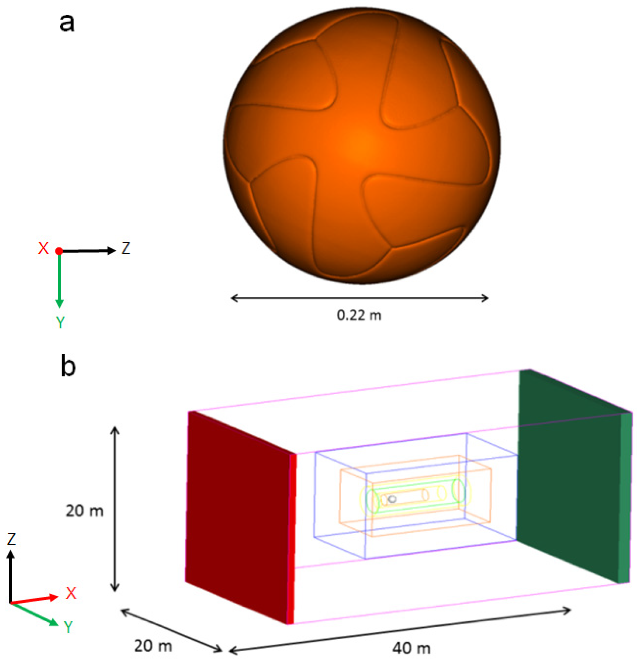
2.1. CFD Analysis Using the Lattice Boltzmann Method

A three-dimensional soccer ball model was constructed (Figure 1a) from data obtained by scanning a real soccer ball (Brazuca, Adidas) using a three-dimensional laser scanner (AICON 3D, Breuckmann GmbH, Germany). For a spinning ball, the flow speed at the velocity inlet was set to 28 m/s (Reynolds number (Re) = 4.25 × 10⁵), and the spinning rates of the ball were defined as 25.1, 50.2, and 75.4 rad/s (4, 8, and 12 rps); the cases corresponding to these spinning rates were denoted as Spin A, Spin B, and Spin C, respectively in this study. For a nonspinning ball, the flow speeds at the velocity inlet were set to 8.2 m/s (Re = 1.25 × 10⁵), 19.0 m/s (Re = 2.8 × 10⁵), and 27.0 m/s (Re = 4.0 × 10⁵); the cases corresponding to these flow speeds were denoted as Nonspin A, Nonspin B, and Nonspin C, respectively. The flow speeds (ball speeds) in this experiment were based on those observed in actual soccer games [23]. A Cartesian grid was adopted to generate a spatial grid with dimensions of 20 m × 20 m × 40 m (W × H × L) comprising nearly 500 million cells (Figure 1b). A sectional grid scale technique was used in this study with a minimum scale of 1 mm and a maximum scale of 4 mm for the cases involving a spinning ball. For the cases involving a nonspinning ball, we defined minimum scales of 1.63 × 10⁻⁴ mm at Re = 1.25 × 10⁵, 7.13 × 10⁻⁵ mm at Re = 2.80 × 10⁵, and 5.02 × 10⁻⁵ mm at Re = 4.00 × 10⁵, and a maximum scale of 4 mm. This grid structure could not represent detailed vortex formations perfectly, but it was used because of computational resource constraints [31]. The outlet pressure was defined as 1013.25 hPa (i.e., atmospheric pressure). The boundary wall of the soccer ball was assumed to obey a no-slip condition, and the outer walls (including the ground surface) were defined as slip walls. The time step for the calculation was 1.018 × 10⁻⁵ s for the cases involving a nonspinning ball and 2.037 × 10⁻⁴ s for the cases involving a spinning ball. In this study, aerodynamic simulations were performed using the incompressible flow model of commercial CFD software (PowerFLOW 5.1, Exa Corp., USA) based on the lattice Boltzmann method [26]. The behavior of many-particle kinetic systems can be expressed in terms of the basic mechanical laws governing single-particle motions at the molecular scale. The Boltzmann equation formulates the problem in terms of a distribution function f (x,v,t), which is the number density of molecules at position x and speed v at time t [32]. The equation (in the absence of external forces) can be written as
D f D t = f ( x ,   v ,   t ) t + v   f ( x ,   v ,   t ) = C ( x ,   v ,   t )
Here, the total derivative on the left-hand side represents the convective motion of particles, whereas the right-hand side expresses complex intermolecular interactions (collisions). Integration of the distribution function makes it possible to obtain macroscopic variables such as fluid density, speed, and pressure.
The collision operator’s main purpose is to drive the velocity distribution function towards its equilibrium distribution. The Bhatnagar, Gross and Krook (BGK) collision operator [32] can then be defined as
C ( x ,   v ,   t ) = 1 τ   [   f ( x , v , t ) f e q ( x ,   v ,   t )   ]
where τ is the relaxation time of the fluid, and f e q ( x ,   v ,   t ) is the equilibrium distribution function.
To solve these equations efficiently, we discretized them on a three-dimensional cubic lattice using the D3Q19 model [32]. This model discretized the velocity space into 19 discrete speeds. The discrete LB equation, using a specific finite-differencing of time ( Δ t = 1 ) , is written as
f i ( x + c i Δ t ,   t + Δ t ) f i ( x ,   t ) = C i ( x ,   t )
C ( x ,   t ) = 1 τ   [   f i ( x , t ) f i e q ( x ,   t )   ]
A volumetric boundary scheme was chosen as the fluid-structure interaction method. Here, the particle boundary condition was conducted at the surface itself (i.e., on the facets that make up the geometry description). Each of these facets had a set of extruded parallelograms corresponding to the discrete velocity directions.
For the cases involving a spinning ball, the boundary layer was simulated using a sliding mesh model [33]. Turbulence was modeled according to the very large Eddy simulation (VLES) principle [32], which directly simulates resolvable flow scales. Unresolved scales were modeled using the renormalization group form of k–ε equations with proprietary extensions to achieve VLES time-accurate physics. The lattice in this solver was composed of voxels, which are three-dimensional cubic cells. The lattice also included surfels, which are surface elements that occur in areas where the surface of a body intersects with a fluid. For the cases involving a nonspinning ball, direct numerical simulation (DNS) was employed without a turbulent model. The average drag, lift, and side forces acting on the soccer ball model were calculated from the unsteady drag, lift, and side forces over a period of 1.0 s (the calculation ran from 0.2 s to 1.2 s). The following parameters were further calculated from the CFD and experimental data collected over a range of conditions: wind velocity (U); force acting in the opposite direction of the wind (i.e., drag D); force acting perpendicular to the wind direction (i.e., lift L); and force acting sideways (S) (i.e., Magnus force) with respect to the frontal view. The aerodynamic forces determined from CFD and through the experiments were converted into the drag force coefficient (Cd), lift force coefficient (Cl), and side force coefficient (Cs) as follows:
C d = D 1 2 ρ U 2 A
C l =   L 1 2 ρ U 2 A  
C s = S 1 2 ρ U 2 A  
Here, ρ is the density of air (1.2 kg/m3), U is the flow velocity (m/s), and A is the projected area of the soccer ball (given by πR2, where R is the radius of the soccer ball). Cd, Cl, and Cs are measured in the +X, +Z, and +Y directions, respectively.
The ratio of the peripheral velocity to the velocity through the air, Sp, was calculated as
S p = ω R U  
where ω is the angular velocity of the soccer ball (rad/s) and R is the radius of the soccer ball (0.11 m). One-way analysis of variance was used to statistically test the average of the Cs values for the spinning and nonspinning balls. Fast Fourier transform (FFT) analysis was employed to compare the frequency characteristics of Cs.

2.2. Wind Tunnel Test

A low-speed circulating wind tunnel with a six-component balance (maximum wind velocity = 55 m/s; measuring section = 1.5 m × 1.5 m; turbulence level = 0.1%) was employed (Figure 2) to verify the drag force coefficient of the nonspinning ball using CFD. The tests were conducted on a thermally bonded soccer ball with six panels (Brazuca (size 5), Adidas; officially approved for use in international games). The ball was supported at the rear using a sting (fixture) fitted to the six-component wind tunnel balance. The ball was fixed to the sting using an adhesive such that it could not rotate. The ball panel orientation in the wind tunnel experiment was the same as that in the CFD analysis. The flow speeds used in the wind tunnel experiment were in the range of 7–35 m/s (Re = 1.06 × 10⁵ to 5.31 × 10⁵) for the nonspinning ball [19].

2.3. Free-Flight Test

The flow (in the frontal cross-sectional plane) behind a soccer ball during flight was visualized using titanium tetrachloride. The soccer ball was placed directly in front of a soccer goal at a distance of 25 m, and a research participant performed a nonspinning kick with slight rotation (knuckle ball) as well as a side-spinning curled kick aimed at the goal. Both placement kicks were delivered at similar velocities to mimic the conditions in a soccer game. Two high-speed video cameras (Photron SA2, Photron Limited) were set up on one side of and behind the ball trajectory, and photographs were taken at 1000 fps. The ball speed and spin rate were measured using high-speed video images. We defined a ball with a rotation of less than 1 rps as a nonspinning ball and a ball with a rotation of more than 4 rps as a spinning ball [34]. The experimental procedure was as follows. Each soccer ball was brush painted with titanium tetrachloride, placed on a designated spot, and kicked toward the goal. As the ball moved toward the goal, the air flow around it was revealed by white smoke produced by the titanium tetrachloride. Photographs were taken using a high-speed video camera. Finally, the ball was collected and cleaned.

3. Results and Discussion

3.1. Steady Cd and Cs Obtained from CFD

The steady drag force coefficient (average Cd) of a nonspinning soccer ball obtained from CFD was ~0.39 in the subcritical regime of Re = 1.25 × 10⁵, ~0.19 in the supercritical regime of Re = 2.80 × 10⁵, and ~0.14 at Re = 4.00 × 10⁵ (Figure 3). The average Cd of the nonspinning ball obtained in wind tunnel tests was ~0.45 in the subcritical regime of Re = 1.24 × 10⁵ and ~0.18 in the supercritical regime of Re = 2.82 × 10⁵ (the critical Reynolds number was 2.67 × 10⁵ (average Cd = 0.15)), which were close to the average Cd values obtained from CFD. We observed a peculiar spike in the subcritical regime owing to the effect of the irregular surface panel shape on the ball, which can affect turbulent reattachment. The maximum measurement error of the average Cd for verifying the measurement repeatability at the same ball orientation was less than 5% in the subcritical regime, whereas those in the critical and supercritical regimes were lower. Moreover, the maximum measurement error of Cd at different ball orientations was also less than 5% in the subcritical regime, whereas those in the critical and supercritical regimes were lower. It is considered that the entire surface roughness of the ball in this wind tunnel test was not significantly different from that of a conventional 32-panel ball (Vantaggio; the critical Reynolds number is 2.20–2.50 × 10⁵) as the total bond length of the six-panel ball used in this wind tunnel test is similar to that of the conventional ball [35,36].
Our experimental setup could not measure the average Cd and Cs of the spinning ball. Therefore, the average Cd and Cs of the spinning ball obtained from CFD were verified using the experimental results reported in a previous study in which a soccer ball with 14 panels was used (Teamgeist (size 5); the critical Reynolds number of the ball was 2.6 × 10⁵) [19]. The average Cd of a spinning ball obtained from CFD was ~0.28 at spin parameter (Sp) of 0.1, ~0.34 at Sp of 0.2, and ~0.36 at Sp of 0.3 (Figure 4a). The average Cd tended to increase as Sp increased. These values were slightly larger than the average Cd of the spinning ball obtained in wind tunnel tests [19]. The average side force coefficient (average Cs) of the spinning ball obtained from CFD was ~0.22 at Sp of 0.1, ~0.28 at Sp of 0.2, and ~0.30 at Sp of 0.3 (Figure 4b). The average Cs also tended to increase as Sp increased, and the values were similar to the average Cs of the spinning ball obtained in wind tunnel tests [19].
The average Cd of the nonspinning ball obtained from CFD in this study is similar to that obtained from wind tunnel tests in the present study as well as in previous studies [19,20] and, hence, it is reasonable to conclude that the CFD calculations are valid. Further, the average Cs of the spinning ball obtained from CFD is slightly larger than the value obtained in wind tunnel tests in this study, but the trends are similar in that the average Cs increases with an increase in Sp. Some reports [34,37] have claimed that the average Cs of the spinning ball increases as Re increases, and considering that the average Cs depends on the ball speed, these calculations may be deemed to be within the permissible range. Thus, the CFD results for the nonspinning and spinning balls in this study are in broad agreement with the results of wind tunnel tests and can be considered reliable.

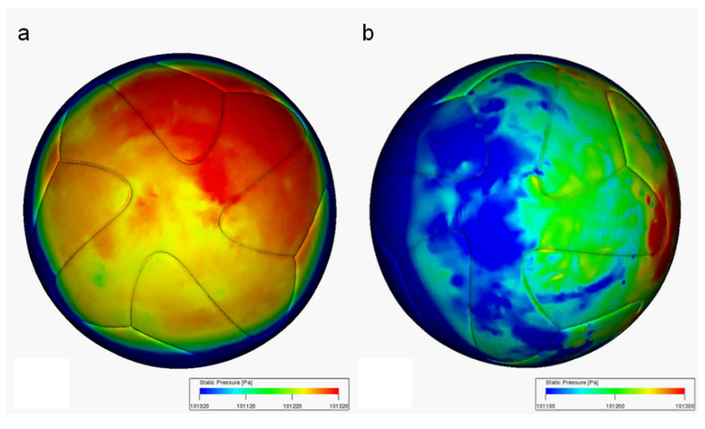
3.2. Flow Visualization from CFD

The boundary layer separation points (line) and pressure distribution in the case of Nonspin B of a nonspinning ball (ω = 0 rad/s, Re = 2.80 × 10⁵) fluctuated irregularly along the time axis, and the accompanying ball wake streamlines also exhibited a deflecting tendency (Figure 5a). In addition, a large-scale counter-rotating vortex pair was very often formed in the wake of the ball (Figure 5b,c), and the position of the vortex pair changed as the separation points and pressure distribution fluctuated. The other cases—Nonspin A and Nonspin C—showed similar trends. It is considered that the simulations did not accurately model the separation and reattachment phenomena, although the separation point in the case of the subcritical regime (Nonspin A) shifted to the stagnation point of the ball.
On the other hand, the boundary layer separation points and pressure distribution in the case of Spin B of a spinning ball (ω = 50.2 rad/s, Re = 4.25 × 10⁵) deflected under the influence of rotation, and the accompanying ball wake streamlines also exhibited a deflecting tendency (Figure 6a,b). Similar to the case of a nonspinning ball, a large-scale counter-rotating vortex pair was observed in the wake, but no large fluctuations were seen, and the pair largely remained at the same position (Figure 6c). The other cases—Spin A and Spin C—exhibited similar trends.
The asymmetry in the flow direction of the separation points (line) in the abovementioned boundary layers of the ball affected the pressure distribution (Figure 7a,b) and vortex structure, resulting in the side and lift forces acting on the ball [23]. In addition, it is considered that the large-scale counter-rotating vortex pair produced traces of deflection in the separation points and pressure distribution, and the vortex structure may be similar to that of a wing tip [38,39].
In the near wake structure of the ball obtained from the back view using CFD, a large-scale counter-rotating vortex pair was formed in the wake of the nonspinning ball (Nonspin B; ω = 0 rad/s, Re = 2.80 × 10⁵), and unstable movements such as rotation around the axis of travel, breakdown [40,41], and re-formation [42] could be observed (Figure 8a–c). Similar trends were observed in the other cases involving a nonspinning ball. In the free-flight test, a large-scale counter-rotating vortex pair was observed in the wake of the nonspinning ball (ω = 5 rad/s, Re = 4.10 × 10⁵) (Figure 8d–f)). The counter-rotating vortex pair exhibited fluctuations with highly unstable movements such as rotation around the axis of travel or breakdown, similar to the cases in the CFD analysis.
In the case of a spinning ball, the CFD results (Spin B; ω = 50.2 rad/s, Re = 4.25 × 10⁵) indicated a large-scale counter-rotating vortex pair in the wake downstream of the rotating direction (right side of the back view in Figure 8), but the vortex pair remained relatively stable and exhibited only minor fluctuations (Figure 8g–i). Similar trends were observed in the other cases involving a spinning ball. In the free-flight test, a large-scale counter-rotating vortex pair, similar to that observed in the CFD analysis, was formed in the wake of the spinning ball (ω = 37.7 rad/s, Re = 3.94 × 10⁵) on the downstream side of the rotating direction (counterclockwise when viewed from the top). Again, this vortex pair structure was relatively stable and had relatively minor fluctuations (Figure 8j–l).
Various vortex structures containing a large-scale counter-rotating vortex have been observed in the wake of a smooth sphere, such as a horseshoe vortex, an alternating vortex, or a hairpin vortex [14,15,16,17]. In addition, a large-scale vortex pair has been observed in wind tunnel tests conducted on nonspinning baseballs [10] and soccer balls [43]. The results of the CFD and free-flight experiments in this study also show a large-scale vortex pair in the wake of nonspinning and spinning soccer balls. Therefore, it can be concluded that a large-scale counter-rotating vortex pair is one of the dominant vortex structures in the wake of nonspinning and spinning soccer balls in flight based on these results.

3.3. Unsteady Cd, Cs, and Cl Obtained using CFD

The unsteady Cs and Cl of a nonspinning ball in the case of Nonspin B obtained using CFD (Re = 2.80 × 10⁵) exhibited bigger large-scale fluctuations than unsteady Cd (Figure 9a). The unsteady Cs and Cl in the case of Nonspin B yielded negative and positive values in 1 s. However, Cs, Cl, and Cd for a spinning ball in the case of Spin B (Sp = 0.2 (8 rps) and Re = 4.1 × 10⁵ (28 m/s)) exhibited small large-scale fluctuations (Figure 9b). In particular, the large-scale fluctuation of the unsteady Cs for a spinning ball was smaller than that for a nonspinning ball. Moreover, the unsteady Cs in the case of Spin B yielded only positive values in 1 s. The unsteady Cs of the nonspinning and spinning balls in the other cases exhibited the same trends.
The average unsteady Cs of the nonspinning ball was 0.054 (s.d. = 0.078) in the case of Nonspin A, 0.039 (s.d. = 0.090) in the case of Nonspin B, and 0.034 (s.d. = 0.050) in the case of Nonspin C (Figure 10). In contrast, the average unsteady Cs of the spinning ball was 0.222 (s.d. = 0.046) in the case of Spin A, 0.282 (s.d. = 0.036) in the case of Spin B, and 0.301 (s.d. = 0.048) in the case of Spin C (Re = 4.25 × 10⁵ in all the cases). The average unsteady Cs of the spinning ball was significantly larger than that of the nonspinning ball (p < 0.01). FFT analysis indicated that the peak amplitudes of Cs in the cases involving a nonspinning ball were located in the frequency range from ~2 Hz to ~5 Hz (Figure 11). On the other hand, in the cases involving a spinning ball, the location of the peak amplitude of Cs was unclear and the results indicated the presence of a strong direct current component in Cs.
According to the above results, Cs of a nonspinning soccer ball fluctuates with greater irregularity with a change in its direction (change in sign) (from ~2 Hz to ~5 Hz), but Cs of a spinning soccer ball fluctuates only slightly in either direction or size and remains relatively stable. The stability of Cs of a spinning soccer ball is presumably caused in part by the suppression of fluctuations in the shifting separation points owing to the rotation of the ball.
It has been reported that the power spectral data of a circular cylinder in the subcritical regime exhibit strong peaks associated with the common vortex shedding frequency, both in the near-wake and the surface measurements, which are in good agreement with the Strouhal number data [44]. As the Reynolds number approaches the critical regime, the increasingly energetic boundary layer is known to be less sensitive to flow fluctuations; hence, the associated line of flow separation on the cylinder surface exhibits a weak oscillating pattern [44]. We speculate that a similar phenomenon may occur on an actual free flight soccer ball.
The results of this study show that although a spinning soccer ball is deflected by shifting of the boundary layer separation points (including the Magnus effect), the flight trajectory of the ball is regular and stable, and hence, a curled shot or pass can be aimed precisely at the outset of its course. In addition, this result is also helpful from the perspective of the goalkeeper because he/she can easily judge and quickly react to the course of the ball.

4. Conclusions

In this study, we examined the aerodynamic characteristics and wake vortex structure of nonspinning and spinning soccer balls using a combination of the lattice Boltzmann method, wind tunnel tests, and free-flight experiments. A large-scale counter-rotating vortex pair was frequently observed in the wake of the nonspinning and spinning balls, and this vortex pair was considered to be a dominant vortex structure in the wake of the balls. In addition, although the separation point fluctuations for the nonspinning ball were large and Cs fluctuated more irregularly with a change in its direction (change in sign), the separation points of the spinning ball fluctuated only slightly, which indicated the tendency of Cs to be relatively stable. Hence, it seems that when soccer balls are kicked, spinning soccer balls are more likely to be precise in terms of the flight trajectory than nonspinning soccer balls. The present study used VLES and DNS for CFD analysis of spinning and nonspinning balls, respectively. However, the Kolmogorov minimum vortex scale [31] was not calculated because of the limitation of computing resources. In addition, the vortex structures and their stability should be examined in more detail; hence, further studies using more powerful computing resources and higher-resolution analysis models are required.

Author Contributions

Conceptualization, S.H., Y.N., N.A. and T.A.; methodology, S.H., Y.N., N.A. and T.A.; software, T.A.; validation, S.H. and T.A.; formal analysis, S.H. and T.A.; investigation, S.H., Y.N., N.A. and T.A.; resources, S.H. and T.A.; data curation, S.H. and T.A.; writing—original draft preparation, S.H. and T.A.; writing—review and editing, Y.N., N.A. and T.A.; visualization, S.H. and T.A.; supervision, S.H. and T.A.; project administration, T.A.; funding acquisition, S.H. and T.A. All authors have read and agreed to the published version of the manuscript.

Funding

This research was funded by the Ministry of Education, Culture, Sports, Science and Technology of the Japanese government, JSPS KAKENHI grant number 20H04066.

Conflicts of Interest

The authors declare no conflict of interest.

References

  1. Thomson, J.J. The dynamics of a golf ball. Nature 1910, 85, 2151–2157. [Google Scholar]
  2. Mehta, R.D.; Bentley, K.; Proudlove, M.; Varty, P. Factors affecting cricket ball swing. Nature 1983, 303, 787–788. [Google Scholar] [CrossRef]
  3. Davies, J.M. The aerodynamics of golf balls. J. Appl. Phys. 1949, 20, 821–828. [Google Scholar] [CrossRef]
  4. Bearman, P.W.; Harvey, J.K. Golf ball aerodynamics. Aeronaut. Q. 1976, 27, 112–122. [Google Scholar] [CrossRef]
  5. Watts, R.G.; Sawyer, E. Aerodynamics of a knuckleball. Am. J. Phys. 1975, 43, 960–963. [Google Scholar] [CrossRef]
  6. Watts, R.G.; Ferrer, R. The lateral force on a spinning sphere: Aerodynamics of a curveball. Am. J. Phys. 1987, 55, 40–44. [Google Scholar] [CrossRef]
  7. Štěpánek, A. The aerodynamics of tennis balls: The topspin lob. Am. J. Phys. 1988, 56, 138–142. [Google Scholar] [CrossRef]
  8. Wei, Q.; Lin, R.; Liu, Z. Vortex-induced dynamics loads on a non-spinning volleyball. Fluid Dyn. Res. 1988, 3, 231–237. [Google Scholar] [CrossRef]
  9. Mehta, R.D. Aerodynamics of sports balls. Annu. Rev. Fluid Mech. 1985, 17, 151–189. [Google Scholar] [CrossRef]
  10. Higuchi, H.; Kiura, T. Aerodynamics of knuckleball: Flow-structure interaction problem on a pitched baseball without spin. J. Fluid. Struct. 2012, 32, 65–77. [Google Scholar] [CrossRef]
  11. Hong, S.; Asai, T.; Seo, K. Visualization of air flow around soccer ball using a particle image velocimetry. Sci. Rep. 2015, 5, 15108. [Google Scholar] [CrossRef] [Green Version]
  12. Achenbach, E. Vortex shedding from spheres. J. Fluid Mech. 1974, 62, 209–221. [Google Scholar] [CrossRef]
  13. Saffman, P.G. Vortex Dynamics; Cambridge University Press: Cambridge, UK, 1992; ISBN 0960-2933. [Google Scholar]
  14. Leweke, T.; Dizès, S.L.; Williamson, C.H.K. Dynamics and instabilities of vortex pairs. Annu. Rev. Fluid Mech. 2016, 48, 1–35. [Google Scholar] [CrossRef] [Green Version]
  15. Widnall, S.E. The stability of a helical vortex filament. J. Fluid Mech. 1972, 54, 641–663. [Google Scholar] [CrossRef]
  16. Taneda, S. Visual observations of the flow past a sphere at Reynolds numbers between 104 and 106. J. Fluid Mech. 1978, 85, 187–192. [Google Scholar] [CrossRef]
  17. Makita, H. Forefront of wind-tunnel experiment on turbulence structure. J. Fluid Sci. Technol. 2007, 2, 525–534. [Google Scholar] [CrossRef] [Green Version]
  18. Sengupta, K.T.; Singh, N.; Suman, V.K. Dynamical system approach to instability of flow past a circular cylinder. J. Fluid Mech. 2010, 656, 82–115. [Google Scholar] [CrossRef]
  19. Asai, T.; Seo, K.; Kobayashi, O.; Sakashita, R. Fundamental aerodynamics of the soccer ball. Sports Eng. 2007, 10, 101–109. [Google Scholar] [CrossRef]
  20. Passmore, M.; Spencer, A.; Tuplin, S.; Jones, R. Experimental studies of the aerodynamics of spinning and stationary footballs. Proc. Inst. Mech. Eng. Part C J. Mech. Eng. Sci. 2008, 222, 195–205. [Google Scholar] [CrossRef] [Green Version]
  21. Goff, J.E.; Smith, W.H.; Carré, M.J. Football boundary-layer separation via dust experiments. Sports Eng. 2011, 14, 139–146. [Google Scholar] [CrossRef]
  22. Carré, M.J.; Asai, T.; Akatsuka, T.; Haake, S.J. The curve kick of a football II: Flight through the air. Sports Eng. 2002, 5, 183–192. [Google Scholar] [CrossRef]
  23. Kray, T.; Franke, J.; Frank, W. Magnus effect on a rotating soccer ball at high Reynolds numbers. J. Wind Eng. Ind. Aerodyn. 2014, 124, 46–53. [Google Scholar] [CrossRef]
  24. Barber, S.; Chin, S.B.; Carré, M.J. Sports ball aerodynamics: A numerical study of the erratic motion of soccer balls. Comput. Fluids 2009, 38, 1091–1100. [Google Scholar] [CrossRef] [Green Version]
  25. Jalilian, P.; Kreun, P.K.; Makhmalbaf, M.M.; Liou, W.W. Computational aerodynamics of baseball, soccer ball and volleyball. Am. J. Sports Sci. 2014, 2, 115–121. [Google Scholar] [CrossRef] [Green Version]
  26. Chen, H. Volumetric formulation of the lattice Boltzmann method for fluid dynamics: Basic concept. Phys. Rev. E 1998, 58, 3955–3963. [Google Scholar] [CrossRef]
  27. Fares, E.; Nölting, S. Unsteady flow simulation of a high-lift configuration using a lattice Boltzmann approach. In Proceedings of the 49th AIAA Aerospace Sciences Meeting Including the New Horizons Forum and Aerospace Exposition, Orlando, FL, USA, 4–7 January 2011; American Institute of Aeronautics and Astronautics: Reston, VA, USA, 2011. AIAA 2011-869. [Google Scholar] [CrossRef]
  28. Chen, S.; Doolen, G.D. Lattice Boltzmann method for fluid flows. Annu. Rev. Fluid Mech. 1998, 30, 329–364. [Google Scholar] [CrossRef] [Green Version]
  29. Cortelezzi, L.; Karagozian, A.R. On the formation of the counter-rotating vortex pair in transverse jets. J. Fluid Mech. 2001, 446, 347–373. [Google Scholar] [CrossRef] [Green Version]
  30. Devenport, W.J.; Rife, M.C.; Liapis, S.I.; Follin, G.J. The structure and development of a wing-tip vortex. J. Fluid Mech. 1996, 312, 67–106. [Google Scholar] [CrossRef]
  31. Kolmogorov, A.N. The local structure of turbulence in incompressible viscous fluid for very large Reynolds numbers. Proc. R. Soc. A Math. Phys. Eng. Sci. 1991, 434, 9–13. [Google Scholar] [CrossRef]
  32. Kotapati, R.; Keating, A.; Kandasamy, S.; Duncan, B.; Shock, R.; Chen, H. The lattice-Boltzmann-VLES method for automotive dynamics simulation, a review. SAE Tech. Pap. 2009, 26, 57. [Google Scholar] [CrossRef]
  33. Sun, C.; Zhang, R.; Chen, H. A PDE Sliding Mesh Algorithm for Turbulent Flow Simulations with PowerFLOW; Technical report EXA Corporation: Boston, MA, USA, 2009. [Google Scholar]
  34. Passmore, M.; Tuplin, S.; Stawski, A. The real-time measurement of football aerodynamic loads under spinning conditions. Proc. Inst. Mech. Eng. Part P J. Sports Eng. Technol. 2017, 231, 262–274. [Google Scholar] [CrossRef] [Green Version]
  35. Asai, T.; Seo, K. Aerodynamic drag of modern soccer balls. Springer Plus 2013, 2, 171. [Google Scholar] [CrossRef] [PubMed] [Green Version]
  36. Hong, S.; Asai, T. Effect of panel shape of soccer ball on its flight characteristics. Sci. Rep. 2014, 4, 5068. [Google Scholar] [CrossRef] [PubMed]
  37. Passmore, M.; Rogers, D.; Tuplin, S.; Harland, A.; Lucas, T.; Holmes, C. The aerodynamic performance of a range of FIFA-approved footballs. Proc. Inst. Mech. Eng. Part P J. Sports Eng. Technol. 2012, 226, 61–70. [Google Scholar] [CrossRef] [Green Version]
  38. Goverdhan, R.N.; Williamson, C.H.K. Vortex induced vibrations of a sphere. J. Fluid Mech. 2005, 531, 11–47. [Google Scholar] [CrossRef]
  39. Asai, T.; Kamemoto, K. Flow structure of knuckling effect in footballs. J. Fluid. Struct. 2011, 27, 727–733. [Google Scholar] [CrossRef] [Green Version]
  40. Benjamin, B. Theory of the vortex breakdown phenomenon. J. Fluid Mech. 1962, 14, 593–629. [Google Scholar] [CrossRef]
  41. Lucca-Negro, O.; O’Doherty, T. Vortex breakdown: A review. Prog. Energy Combust. Sci. 2001, 27, 431–481. [Google Scholar] [CrossRef]
  42. Ortega, J.M.; Bristol, R.L.; Savaş, Ö. Experimental study of the instability of unequal-strength counter-rotating vortex pairs. J. Fluid Mech. 2003, 474, 35–84. [Google Scholar] [CrossRef]
  43. Mizota, T.; Kurogi, K.; Ohya, Y.; Okajima, A.; Naruo, T.; Kawamura, Y. The strange flight behaviour of slowly spinning soccer balls. Sci. Rep. 2013, 3, 1871. [Google Scholar] [CrossRef]
  44. Capone, A.; Klein, C.; Felice, F.D.; Miozzi, M. Phenomenology of a flow around a circular cylinder at subcritical and critical Reynolds numbers. Phys. Fluids 2016, 28, 74101. [Google Scholar] [CrossRef]
Figure 1. (a) Three-dimensional soccer ball model obtained by laser scanning and (b) the Cartesian grid used to generate a spatial grid (W 20 m × H 20 m × L 40 m) for computational fluid dynamics (CFD) analysis. The flow is from the left to the right.
Applsci 10 04543 g001
Figure 2. Set up of wind tunnel experiment.
Applsci 10 04543 g002
Figure 3. Comparison of the drag force coefficients of a nonspinning ball determined from CFD analyses and wind tunnel tests (the error bars indicate the standard deviation of Cd).
Applsci 10 04543 g003
Figure 4. Comparison of (a) drag force coefficients and (b) side force coefficients of a spinning ball determined from CFD analyses and wind tunnel tests.
Applsci 10 04543 g004
Figure 5. Example of static pressure and x-vorticity seen on streamlines around a nonspinning soccer ball obtained using CFD from (a) side view, (b) top view, and (c) back view.
Applsci 10 04543 g005
Figure 6. Example of static pressure and x-vorticity observed on streamlines around a spinning soccer ball using CFD from (a) side view, (b) top view, and (c) back view.
Applsci 10 04543 g006
Figure 7. Example of static pressure observed on (a) nonspinning and (b) spinning soccer balls using CFD (back view). The spin direction of the spinning soccer ball in (b) is anticlockwise from the top view.
Applsci 10 04543 g007
Figure 8. Flow visualization of nonspinning soccer balls using (a–c) CFD and (d–f) free-flight tests, and that of spinning soccer balls using (g–i) CFD and (j–l) free-flight tests. The ball spins with a positive rotation about the Z-axis. The Re values for the nonspinning and spinning balls are 2.80 × 10⁵ and 4.25 × 10⁵ (spin rate = 8 rps), respectively. In the CFD results, the color of the surface of the soccer ball varies according to the pressure coefficient, whereas the color of the streamlines varies according to the vorticity. The view is from behind the ball (back view).
Applsci 10 04543 g008
Figure 9. Drag, side, and lift force coefficients of (a) nonspinning soccer ball for Re = 2.80 × 10⁵ and (b) spinning soccer ball for Re = 4.25 × 10⁵ (spin rate = 8 rps) obtained using CFD.
Applsci 10 04543 g009
Figure 10. Comparison of the average side force coefficients (Cs) of nonspinning and spinning soccer balls (p < 0.01). The Re values in the case of Nonspin A, Nonspin B, and Nonspin C are 1.25 × 10⁵, 2.80 × 10⁵, and 4.00 × 10⁵, respectively, and the Re values in the case of Spin A, Spin B, and Spin C are 4.25 × 10⁵ (spin rate = 4, 8, and 12 rps, respectively).
Applsci 10 04543 g010
Figure 11. Amplitude of Cs obtained from fast Fourier transform (FFT) analysis in the cases involving (a) nonspinning and (b) spinning balls.
Applsci 10 04543 g011

