Abstract
In this work, four different semi-active controllers for a quarter of vehicle and full vehicles are evaluated and compared when used in internal combustion engine (ICE) vehicles vs electric vehicles (EVs) with in-wheel motor configuration as a way to explore the use of semi-active suspension systems in this kind of EVs. First, the quarter of vehicle vertical dynamics is analyzed and then a full vehicle approach explores the effectiveness of the control strategies and the effects of the traction in the vertical Control performances. Aspects like the relation between traction and suspension performances, and the resonance frequencies are also discussed.
Keywords:
in-wheel; semi-active; suspensions; EVs; automotive; control; switched; reluctance; motor; SR 1. Introduction
Today, automotive vehicles are considered the primary conveyance due to the high amount of people, which performs its daily activities making use of them. For that, continuous improvements focused on safety and travel experience may be reached. During the last years, these improvements have been devoted to enhancing automotive suspension systems, where the road holding as well as the comfort for vehicle’s passengers have been improved. A balance between road holding and comfort has been the main goal in this area, however, most of the devoted work has been focused on internal combustion engine vehicles. For this reason, with the high and growing adoption of the EVs, there is a need for solutions for guaranteeing the balance between road comfort and holding especially when working with an in-wheel powertrain configuration with semi-active suspension systems when a switched reluctance motor (SRM) is employed. The use of SRM instead of brushless DC (BLDC) motors in in-wheel configurations has increased due to the low cost, efficient power transfer, high torque density and direct drivetrain system features that the SR motors offer for this application [1].
In the last years, some solutions in automotive suspension systems aimed to reduce vibration effects in in-wheel EVs have been reported. In Nagaya et al. [2], the in-wheel electric motor is employed as an “Advanced-Dynamic-Damper-Motor” (ADM), where the electric motor is considered as a damper mass in order to decrease tire contact force fluctuation in the vehicle. This achievement was accomplished by attaching the motor in the unsprung mass by employing a spring and damper of exclusive use, Figure 1a). As a result, the vibration of the sprung mass decreased. In Ma et al. [3], the ADM and an LQR active suspension systems are considered for sprung mass vibration reduction but also a vertical linear force () provided by the switched reluctance (SR) in-wheel electric motor is taken into account for the analysis of the vertical dynamics. In Wang et al. [4], an FxLMS (filtered-X-least mean square) is proposed for improving suspension performance with an active suspension system. In this case, the electric motor is considered as part of the unsprung mass, and the is also considered as an extra force adding vibration to the unsprung mass. The FxLMS controller is able to generate a controllable force for suppressing the vibration generated by . In Shao [5], the ADM complemented by an active suspension system is employed, where the suspended motor and suspension parameters are optimized based on genetic algorithms (GA) and are complemented by an LQR controller for the active suspension system. Something similar occurs in Shao et al. [6], where the ADM is complemented by a fault-tolerant fuzzy taking into account actuator faults and control inputs restrictions. The dynamic force transmitted to the in-wheel motor is taken as an additional controlled output as a way for reducing motor wear. In Liu et al. [7], a two-stage optimization control method is proposed to improve ADM performance. Where an LQR based on Particle Swarm Optimization (PSO) is designed for mitigating the in-wheel electric motor vibration and a finite-frequency controller is designed for the active suspension. Obtaining, as a result, a method which is able to improve the ride comfort and mitigates in-wheel motor vibration. Li et al. [8] consider the stator (housing) of the in-wheel electric motor as the unsprung mass and the rotor as an extra mass in the in-wheel vehicle dynamic model, Figure 1b). In this work, a multi-objective optimization control method of active suspension for solving the negative vibration issues generated by is presented. The PSO method is employed for obtaining active suspension system optimal parameters. The results show that the optimized suspension system is able to reduce the effects of . In Zhu et al. [1], the vibrations given by the switched reluctance motor (SRM) are analyzed, and some control strategies which consider the vertical acceleration of the chassis as a control objective are proposed as a way of mitigating them. At the end, a switchable controller based on the proposed strategies is given as a way for guaranteeing the best performance for each driving condition tested. As can be seen, the current work in suspension systems for in-wheel electric vehicles is focused on active suspension systems, which demands more energy consumption as well as instrumentation.
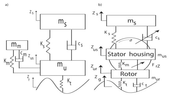
Figure 1.
(a) Advanced-Dynamic-Damper-Motor (ADM), (b) In-wheel quarter of vehicle (QoV) three masses.
From control of semi-active suspension systems in ICE vehicles in the last years, it can be said that the Fuzzy [9,10,11,12,13], Sky-Hook [14,15,16], and Ground-Hook [17,18] control strategies, as well as, their variations have been the most employed techniques for satisfying the main semi-active suspensions control objectives. In these semi-active approaches, the most common control output has been the desired damping force that later is converted to current in order to manipulate the MR but in some cases, as in References [13,19], where the control output is already current. The most employed control inputs are the speeds of the sprung and unsprung mass as well as the real time displacements. For the controllers validation through simulation, it is common to employ Matlab/Simulink [11,12,13], Carsim [19,20], Bikesim [21], Trucksim. All these programs require the parameters of the vehicle’s suspension, and a road disturbance profile to generate results. Most of the reported results refer to time tests, where the road profile is a step or bump-like signals, and/or frequency evaluations with white noise or sinusoidal signals are representing the road profile. Moreover, Typically, the quantitative performance evaluation is performed with root mean square (RMS) values in the time domain as in Reference [9], and power spectral density (PSD) in the frequency domain [22]. For qualitative assessments, the objective is to improve the performance achieved with a passive as much as possible.
For the experimental validation of the controller it is possible to employ an experimental quarter of vehicle (Exp-QoV) [16], Hardware in the Loop (HiL) [23,24,25,26] or a Vehicle (Exp-V) [27], where accelerometers and sensors are employed to obtain the information that will be processed by the controller in order to achieve the main objectives of the control strategy.
In this work four different semi-active controllers as well as two current levels for QoVs and full vehicles are implemented in ICE and electric vehicles with and without considering the unbalanced vertical force given by the SRM. The performances are compared as a way for visualizing how is the suspension objectives improvement varying between the ICE and electric models. For the QoV case study, the simulations are carried out in MATLAB/Simulink. While for the full vehicle, software in the loop (SiL) tests are performed in MATLAB/Simulink and Carsim.
2. Methods
2.1. A Semi-Phenomenological (SP) Model of a Magnetorheological Damper
For simulation tests, a semi-phenomenological (SP) model, that comprises the hysteresis loop of the MR damper, is considered. This MR damper model was proposed in Reference [20], and it considers an hyperbolic tangent and the proportional effect of manipulation are employed in order to shape the sigmoidal diagram when the manipulation variable is different from . This SP model is given by the following equations:
where is the MR damping force (compounded by and ), is the passive force (damping force when current is equal to 0A) and is the force due to the magnetorheological effect of the damper in the presence of electric current, is the damping coefficient, is the stiffness coefficient, is the friction coefficient, , and define the sigmoidal behavior of the friction component, , and define the sigmoidal force component due to the MR behavior and is the damping coefficient due to the electric current. Model parameters employed for simulation purposes are shown in Table 1.

Table 1.
Semi-Phenomenological (SP) asymmetric model parameters.
2.2. F-Class Vehicle Model
For simulation purposes, an F-class vehicle is considered (Figure 2). F-class vehicles are known to be vehicles with higher performance, better handling, comfort, more top quality equipment and an stupendous design. Examples of commercial vehicles classified as F-class are: Mercedes S class, Audi A8, and Cadillac DTS. The parameters of the F-class vehicle shown in Table 2 were extracted from the CarSim parameters library.
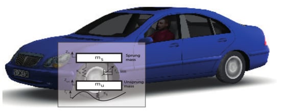
Figure 2.
F-class vehicle, adapted from Carsim.
Table 2.
F-class vehicle parameters in CarSim.
The main parameters of the QoV are the sprung mass (), which corresponds to the vehicle chassis (body) and components supported by the suspension, and the unsprung mass () is compounded by the wheel components (tire, rim, and links). From the sprung mass of the whole vehicle (), the () for the QoV must be estimated by making use of the weight distribution of the vehicle; which can be computed employing the dimensions shown in Figure 3. For the present case study, the sprung mass for the QoV is calculated as follows: . For that, it can be considered that the 60% of the body mass is located at the front part of the vehicle and 40% in the rear part.
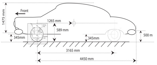
Figure 3.
F-class vehicle physical dimensions.
Knowing that and considering an uniform distribution of the weight at the front (both corners) with two front passengers as well as a mid-level fuel tank, it is possible to estimate the QoV parameters shown in Table 3 for one corner of the F-class vehicle at the front, where represents the tire stiffness which is assumed to be linked to the road (), and the damping effect due the tire is not considered.
Table 3.
Front QoV parameters.
A modified F-class vehicle model is also studied, where an in-wheel electric motor is considered inside each wheel hub instead of a unique internal combustion motor. The parameters in Table 4 are estimated knowing the new mass values, battery bank, and the characteristics of the electric motors taken from Reference [28] (for a general), and from Reference [29] (characterized for a Brabus Electric 4WD Mercedes). The modified QoV parameters are shown in Table 5. The and resonance frequencies were estimated according to Reference [20]. For the in-wheel electric vehicle, a residual vertical force due to the electric motor can be considered for some tests. In this case, the residual vertical force that will be considered is shown in Figure 4 as in Reference [4]. Where it was estimated considering constant speed () and an SRM of 6 poles. The unbalanced vertical force is generated by the rotor eccentricity in the SRM and depends on the electromagnetic excitation. The unbalanced vertical force affects the vertical dynamics as an inertial force and occurs due to the gap shown in Figure 5. Which is given by the fabrication tolerances. As can be seen in Figure 5, has two components, the radial and tangential forces ( and ).
Table 4.
Modified F-class vehicle parameters in CarSim.
Table 5.
Modified front QoV parameters.
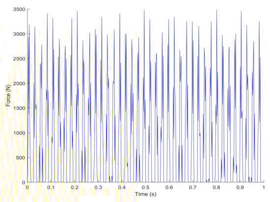
Figure 4.
Residual vertical force.
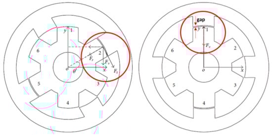
Figure 5.
Switched reluctance motor (SRM) residual vertical force diagram, adapted from Reference [4].
2.3. QoV’s Description
The three different QoV’s—shown in Figure 6—considered for simulation purposes are described in this section.
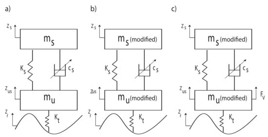
Figure 6.
QoVs for simulation, (a) NQoV, (b) ModQoV (c) ModQoVFv.
The normal QoV (NQoV) shown in Figure 6a corresponds to an ICE vehicle which has a semi-active suspension system and where a sprung and an unsprung mass are considered as in Reference [30]. The modified QoV (ModQoV) shown in Figure 6b corresponds to an in-wheel electric vehicle considering the electric motor as part of the unsprung mass and the battery bank as part of the sprung mass as it was described in Section 2.2. In Figure 6c (ModQoVFv) the same masses than in Figure 6b are considered as well as, the unbalanced vertical force () given by the in-wheel electric motor, as mentioned in Reference [4]. In this case, the active suspension system is replaced by a semi-active one. The mathematical model for the NQoV and ModQoV is given by the following equations:
where and are the sprung and unsprung mass, respectively. and are the stiffness of the damper and tire, respectively. The displacements of the sprung and unsprung mass are given by and , respectively. While the road profile is represented by . The damping force is given by , which is composed of the passive and semi-active components.
On the other hand, the mathematical model for the ModQoVFv which considers is given by:
2.4. Controllers Definition
2.4.1. Sky-Hook (SH)
The SkyHook (SH) (Figure 7a) strategy is the passengers comfort analysis reference point in suspensions control due to its performance, ease of implementation and design [31]. This approach is not intended to improve road holding performance because the sprung mass vibration is not considered in its control law. The control system uses 2 accelerometers, and the speed and relative speed of the sprung are usually estimated. The control law is:
and the damping force () is given by:
where y represent the damping coefficient limits (maximum and minimum, respectively), y are the sprung and unsprung mass speeds, respectively. The Sky Hook performance is limited to low frequencies, and new improvement proposals have been proposed [31].
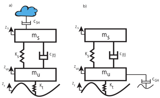
Figure 7.
Heuristic controllers (a) Skyhook (b) Groundhook.
2.4.2. Ground-Hook (GH)
The control strategy known as GroungHook (GH) (Figure 7b) focuses on improving the road holding, and it is presented in Reference [18], where a fictitious element (damper) between the ground and the wheel parallel to the tire is considered. This controller follows a similar principle to the SH but it is oriented to the dynamic tire-forces reduction to guarantee the desired level of road holding. The control law is given by:
and the generated damping force () is given by:
2.4.3. Mix-1-Sensor (M1S)
To reduce instrumentation costs, Savaresi and Spelta [32], developed an experiment to validate the Mix-1 Sensor (M1S) controller performance following the SH-ADD principle employing just one sensor (suspended mass acceleration) obtaining good comfort performance. This algorithm chooses the maximum or minimum damping coefficient at the end of each sample according to the vertical movement of the sprung mass. The control law is:
where is given by the masses resonance frequencies. The damping force () is given by:
2.4.4. Frequency Estimation Based (FEB)
The Frequency Estimation Based (FEB) controller for semi-active suspensions is presented in Reference [19]. For the manipulation signal, the harmonic motion of the damper is considered as well as the piston deflection, and damper deflection velocity. Displacements and speeds are approximated employing RMS values, and the required frequency () is estimated with:
the FEB control law is given by the following criteria:
where I is the current, which will be applied to the semi-active damper. The value for I in each interval is chosen according to the specific requirements, for example, in a control system where the main objective is to reach both comfort and road holding requirements, the following current values are chosen: full current according to the damper’s operation domain (hard damping) in bandwidth intervals that contain the resonance frequencies, and (soft damping) in the remaining intervals. The frequencies and are the bandwidths limits given by:
the first step is to estimate the masses resonance frequencies ( and ) of the QoV employing:
where is the ride rate, is the wheel rate and is the motion ratio of the damper.
2.5. Controllers Tuning for Benchmark
Once the vehicle model is defined, the on/off controllers SH, GH, and the M1S should be tuned. This means that the ideal damping coefficients () for each controller must be approximated as it is mentioned in Reference [19]. is given by Equation (17).
where is the critical damping for the mass (m). The values of the mass (m) and stiffness (k) for the sprung mass are and , while for the unsprung mass, and . The ideal damping force in a QoV suspension can be computed as follows:
By making use of the Equation (17) and QoV parameters of Table 3 and Table 5 the ideal damping values for a corner (front side) of the vehicle are calculated in Table 6. For the and controllers, the output signal is force, and the damper model requires electric current as input for varying the MR damping force. For force to current equivalence, a feedback control as in Reference [20] was implemented as it is shown in Figure 8. For tuning the FEB controller, four bandwidths must be determined according to Reference [20], and employing the resonance frequencies of the masses shown in Table 3 and Table 5 for the normal and the modified QoV, respectively.
Table 6.
Values for damping coefficients computing.
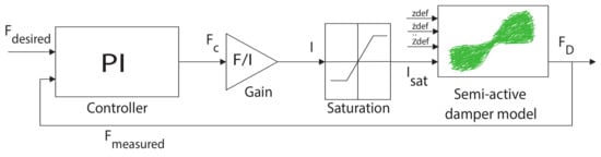
Figure 8.
Force-electric current conversion with PI controller.
The bandwidths for the normal and modified QoV are shown in Table 7 and Table 8 respectively. In the bandwidths where the resonance frequencies are present, hard damping () was considered, while in the rest of bandwidths, soft damping () was chosen. This is the applied approach for guaranteeing a road-holding-comfort oriented suspension.
Table 7.
Frequency Estimation Based (FEB) Frequency bandwidths for the QoV.
Table 8.
FEB Frequency bandwidths for the modified QoV.
The values of and represent the minimum and the maximum current values for manipulating the MR damper, respectively. The equivalence to damping ratio is estimated according to the next equation.
where is the desired gain of the damping value. In this case is considered. k and m are stiffness and mass values. From the Table 1, the values for the and are employed. Which corresponds to the MR damper model. The equivalence current to damping ratio is presented in Table 9.
Table 9.
Current to damping ratio equivalence.
2.6. Input Signals Definition
The input signals definition for the time and frequency domain is done as in Reference [19]. A detailed description of them is shown below.
2.6.1. Time Domain
- Sinusoidal road with resonance frequency. As a way to visualize the comfort and road holding conditions, whose are normally in 1–2 Hz and 10–15 Hz, a comparative work in the body and road holding resonance is performed employing sinusoidal roads. Two sinusoidal signals are considered with mm and mm, respectively, Figure 9. Considering the resonance frequency of the masses for each QoV setup.
 Figure 9. Time domain input signals.
 - Step road. A step road disturbance of magnitude 3 cm is implemented at the time of 2 s. The test duration is 4 s, Figure 9.
2.6.2. Frequency Domain
The evaluation of the automotive semi-active controllers with a nonlinear QoV model is made according to industrial specifications [33,34,35]. A road drive is designed considering the shape of the relative amplitude spectrum of the position command at 10 different points between and 30 Hz, as it is shown in Table 10. Where the 1 in amplitude relative means 15mm. This pattern was considered in order to excite the frequencies of interest maintaining realistic velocities in the shock absorber, Figure 10 [36].
Table 10.
Definition of the relative amplitude spectrum.
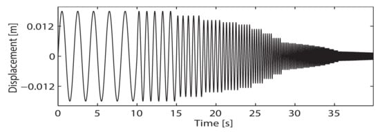
Figure 10.
Frequency domain input signal.
2.7. Full Vehicle Tests Definition
Three tests are considered for evaluating the full vehicle model in CarSim, Figure 11 [37]. The tests are—Bounce Sine Sweep Test (BSST), which is focused on ride comfort and human comfort; the Double Lane Change (DLC) test for handling, and the Fishhook (FSH) test, which is focused on handling and stability. In BSST, the variables of interest are the body vertical acceleration, body vertical displacement, and pitch angle. In the DLC and FSH tests, the variable of interest are—lateral acceleration, roll, yaw rate, vehicle sideslip angle, and roll rate. A description of each test follows:
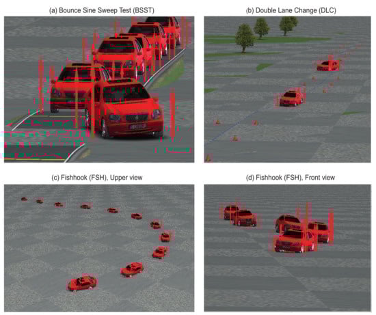
Figure 11.
Implemented tests in CarSim for a full vehicle model.
- Bounce Sine Sweep Test (BSST). The BSST is used in the test of vertical body displacement (heave) and vertical (body) acceleration over a range of frequencies (typically 0–20 Hz), Figure 11a. This helps to ensure that an appropriate suspension tuning is done by exploring suspension performance in a bandwidth, which is expected to be faced in suspension’s useful life [38].
- Double Lane Change (DLC). DLC tests can provide use full information about vehicle’s handling in a highly transient situation. These are avoidance maneuvers commonly seen in real life [39] Figure 11b. This test consists on steering the vehicle through the entrance lane, and suddenly, turns left to avoid the single cone in the second lane, turning right for returning to the original lane, and then straightening the vehicle for leaving the course via the exit lane cones [40].
- Fishhook (FSH). Fishhook maneuver is detailed in the Toyota Engineering Standard TS-A1544. This propose of this procedure is to produce two-wheel lifts by imparting a rapid steering reversal to the vehicle while it is at a maximum lateral acceleration in one direction due to the initial steer. With this test, the vertical acceleration changes to the maximum value in the other direction, as shown in Figure 11c,d. By applying this rapid change in the lateral acceleration a large roll angular momentum to the chassis is applied due to the vehicles leaning at a relatively large angle to one side and then being forced to leaning in the opposite direction [40].
2.8. Controllers Performance Indexes for the QoV
2.8.1. Time Domain
There are 2 different evaluation criteria for temporal tests as well as domain tests, known as qualitative and quantitative. The most applied qualitative evaluation criteria in the time domain are variable temporal test graphics in the variables of:
- Sprung mass vertical acceleration. It is employed for passenger comfort analysis.
- Relative displacement and/or between the two masses. It is employed the suspension deflection analysis.
- Contact force between the road profile and the wheel. It is employed for the road holding analysis.
For a quantitative evaluation, the most employed performance index is the RMS (Root Mean Square) of the sprung mass acceleration () to analyze the comfort. RMS of the unsprung mass acceleration () or to analyze the road holding and RMS of the relative displacement () to assess suspension useful lifetime. The next equation defines the general calculation of an RMS value
where x is the interest signal, and T determines the period of time during the analysis. There are some similar performance indexes, in Reference [9] a reduction rate of the RMS of the semi-active suspension with respect to the passive suspension. The equation is:
where is the variable process deviation reduction index in the time domain.
2.8.2. Frequency Domain
In the frequency domain, the PSD (power spectral density) and the pseudo-bode diagram are considered and described.
The performance of the semi-active suspension can be quantitatively analyzed employing PSD. Poussot-Vassal [22], determines a performance index for each control objective in terms of improving, that is to say, the semi-active system PSD is compared versus the performance of a passive suspension, employing the next equation:
Nassirharand and Taylor [41], proposed an algorithm for evaluating controllers performance in the frequency domain known as pseudo-Bode (PSB) algorithm. A pseudo-bode plot illustrates the evaluated frequencies versus the measured gains in the transfer function. With this algorithm, it is possible to visualize the gains of the interest variables in certain frequencies in order to evaluate comfort and road holding improvement. The PSB algorithm is given by:
- Excite the system employing a sinusoidal signal as an input at the frequency for M periods.
- Measure the output signal (signal of interest).
- Compute the discrete Fourier transform of the input and output signal.
- Compute the magnitudes and .
- Compute the expression:where is the gain to the transfer function for the given frequency .
- The sequence must be repeated M times, each time considering a specific frequency until the desired PSB is achieved.
Four bandwidths of interest are considered as in References [42,43] for visualizing performance improvement.
- BW1: [0–2] Hz range. The main goal is comfort. The resonance frequency of the sprung mass is included.
- BW2: [2–9] Hz range. The main goal is also the comfort. High gains of vertical accelerations in this bandwidth generate overall discomfort by shaking [44].
- BW3: [9–16] Hz range. The main goal is road holding. This bandwidth is known as tirehop BW because it contains the unsprung mass frequency resonance.
- BW4: [16–20] Hz range. This will be named the head injury BW. The main goal is road holding. The dangerous vibration can generate internal damage to the body.
2.9. Controllers Performance Indexes for the Full Vehicle
For these tests, an F-class vehicle with an axis system vehicle-body-fixed system (SAE standard J670e) is considered [45]. When working with a full vehicle, the four corners directly affect vehicle’s motion resulting on heave, pitch, roll and yaw motions. For that, suspension’s behavior of a full vehicle model must be analyzed making use of these variables which are related to human comfort, ride comfort, road holding, vehicle handling, and vehicle roll (Table 11), [37]. The definitions of these concepts are:
Table 11.
Performances to be evaluated in full vehicle model tests.
- Human comfort is defined as the human response to vibration. Vertical acceleration of the heave in a vehicle gives the only reliable subjective-objective correlation and must be considered as the interest value when analyzing human comfort [46].
- Ride comfort requires perfect isolation of the vehicle body from the road disturbances. To reach the ride comfort the magnitude of the heave and pitch of the car body with respect to typical road profiles should be minimized [43].
- Road holding performance is the ability of a car to remain stable when moving and keep contact between the road and tire, especially at high speeds. It is related to the lateral acceleration. High acceleration means poor road holding [47].
- Handling is defined as the percentage of the available friction in tires or as the maximum achievable lateral acceleration employed by the car-driver combination [46]. The most typical measurements are: roll, lateral acceleration, yaw rate, and vehicle sideslip angle [39,48].
- Vehicle roll is presented in the cornering, and during braking maneuvers, it can occur on perfectly smooth roads [49]. The roll rate and roll angle of a vehicle are known as the most important variables when analyzing vehicle roll dynamics [50].
2.10. Simulations and Data Processing Procedure
The process for simulating, processing the data and analyzing the results is summarized in Figure 12. The simulations are performed in the QoV models by varying the current levels (open loop) and control strategies (closed loop) employing the time and frequency domain input signals defined in Section 2.6. After that, the interest variables are processed employing the RMS and PSD algorithms. The results are compared against the baseline suspension. Then, the improvements and gains are plotted and analyzed. For the full vehicle models, the simulations of the tests defined in Section 2.7 are performed employing SiL between Matlab/Simulink and Carsim. The interest variables improvement is visualized employing the RMS index.
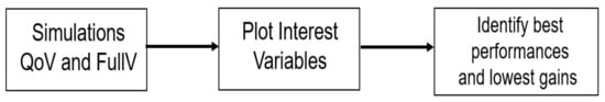
Figure 12.
Simulation and analysis process.
3. Results and Discussion
In this section, the simulation results obtained for the QoVs and full vehicle tests are presented and described.
3.1. QoV
The results are presented in time and frequency domain for the simulations performed in the different types of QoV previously described in Section 2.2. For analyzing the improvement, a baseline suspension is considered. The best cases of improvement for each test and each QoV in open and closed loop tests are presented in Table 12 and Table 13, respectively. Where the bold data correspond to the interest values in each objective (comfort, road holding, and useful lifetime). A decision row is also included, which gives the best current level or controller for enhancing the desired objective on each QoV in accordance with the performance indexes.
Table 12.
QoV Results in open loop.
Table 13.
QoV results in closed loop.
3.1.1. Open Loop
The results in open loop are presented for the normal QoV, the modified QoV (in-wheel electric motor) and the modified QoV (in-wheel electric motor) considering the residual vertical force provided by the electric motor in Figure 13, Figure 14 and Figure 15, respectively.
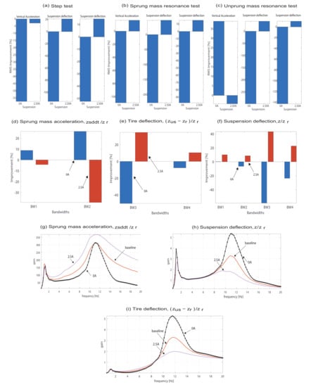
Figure 13.
Results from open loop simulations for the comparison in a nonlinear QoV model considering a baseline suspension.
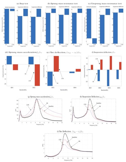
Figure 14.
Results from open loop simulations for the comparison in a nonlinear modified QoV model considering a baseline suspension.
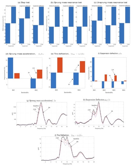
Figure 15.
Results from open loop simulations for the comparison in a nonlinear modified QoV model considering a baseline suspension and the residual vertical force.
For comfort improvement in the NQoV, it is shown that for the step test (Figure 13a), the baseline suspension gives the best comfort improvement, followed by the . While in the sprung mass test (Figure 13b), the enhances comfort performance by , followed by the baseline suspension. In this case, the gives a negative comfort improvement. Besides, in the frequency domain the best improvement is given by the , which gives an improvement of the in accordance with the IPSD (Figure 13d) as well as the lowest gains in the pseudo-bode plot (Figure 13g), where it is also demonstrated that with lower current values (soft suspension), the performance is increased probably related to a high slope in the compression curve of the MR damper. According to this information, it can be said that the gives the best improvement in comfort for the NQoV in open loop. By the side of the road holding, it is improved in the step and unsprung mass tests (Figure 13a,c) by the in and , respectively. Which means that a harder suspension is required for improving the road holding. In the frequency domain, the improvement occurs in the same way, the current increases the road holding in the frequency domain by in accordance with the IPSD (Figure 13e) and gets the best gains in the pseudo-bode plot (Figure 13i) for the tire deflection in the interest bandwidths. That’s why the current level can be considered as the most effective for enhancing the road holding objective in open loop considering as reference a baseline suspension in the NQoV. By the side of the useful lifetime, it is enhanced by the of current in the step, sprung mass and unsprung mass tests (Figure 13a–c) by , and , respectively. Where it can be seen that the damper reduces the suspension deflection when the current level is increased (harder suspension). While with , the useful lifetime is decreased. Likewise, in the frequency domain wherein all the bandwidths, a hard suspension () optimizes the suspension deflection by in accordance with the IPSD (Figure 13f) and gives the lowest gains for the suspension deflection in the pseudo-bode plot (Figure 13h). According to the indexes discussed above, the best useful lifetime improvement is given by the of current for the NQoV in open loop considering as reference a baseline suspension.
For the MQoV, the baseline suspension enhances comfort in the step test (Figure 14a) followed by the . By the side of the sprung mass test (Figure 14b), the improves the comfort in a , and as it can be seen, the performance decreases with a soft suspension. On the other hand, in the frequency domain, the enhances the comfort by a in accordance with the IPSD (Figure 14d) as well as diminishes the vertical acceleration gains in the pseudo-bode plot (Figure 14g), where it can be seen that comfort improvement decreases with when having a harder suspension (higher current values). According to the information described above, it can be said that the current level gives the highest comfort improvement for the MQoV in open loop. By the side of the road holding, the improves it in the step and unsprung mass test (Figure 14a,c) by and , respectively. Where the road holding increases as the current level does (with harder suspensions). Likewise, in the frequency domain, the A improves the road holding in a according to the IPSD (Figure 14e) as well as shows the lowest gains in the pseudo-bode plot (Figure 14i) for tire deflection. Where the road holding is improved when working with a hard suspension () and decreased by employing a soft one (). From this, we can say state that, for guaranteeing a road holding improvement for the MQoV in open loop considering as reference a baseline suspension, the (hard suspension) current level might be employed. In the case of the useful lifetime, a similar situation occurs, for the step, sprung mass and unsprung mass tests (Figure 14a–c), where the enhances the useful lifetime by , , and , respectively. By the side of the frequency domain, occurs almost the same, where a hard suspension () decreases the gains in the pseudo-bode plot for the suspension deflection and increases the IPSD. For the time domain tests, the useful lifetime increases with of current and decreases when working with . In a similar way, in the four bandwidths of the frequency domain, the guarantees an improvement of the useful lifetime according to the IPSD (Figure 14f) and to the pseudo-bode gains from Figure 14h. According to the results described above, the of current (hard suspension) guarantees the useful lifetime improvement for the MQoV in open loop considering as reference a baseline suspension.
In the MQoVFV, the highest comfort improvement () during the step and sprung mass tests (Figure 15a,b) is given by the current level. In both cases, the performance decreases as well as the current does. Besides, in the frequency domain, comfort enhancement is given in a by the in accordance with the IPSD (Figure 15e) as well as with the lower gains from the pseudo-bode plot (Figure 15g). That’s why it can be said that the gives the best improvement for the MQoVFV in open loop is given by the , which probably means that the presence of the unbalanced vertical force, demands a harder suspension for improving comfort. The road holding is improved by and in the step and sprung mass tests (Figure 15a,c), respectively. Where the road holding decreases, the current also does. In the frequency domain it occurs in almost the same way; a higher current guarantees the road holding. The highest road holding improvement is of in accordance with the IPSD (Figure 15e) and is given by the as well as the lowest gains for the tire deflection in the pseudo-bode plot (Figure 15i). The current level gives a negative improvement. According to the performance discussed above, it can be said that a harder suspension () guarantees the road holding in the MQoVFV in open loop. By the side of the useful lifetime the improves it for the step, sprung mass and unsprung mass tests (Figure 15a) by , and , respectively. Whereas in the other QoV models, the useful lifetime increases as the current level does. In the frequency domain it occurs almost the same way; the suspension deflection is enhanced by the in a according to the IPSD (Figure 15f) as well as to the lower gains shown in the pseudo-bode plot (Figure 15h). As can be seen, higher current values guarantee a higher useful lifetime. The best useful lifetime improvement is given by the of current for the MQoVFV in open loop considering as reference a baseline suspension.
For the comfort in the NQoV, the M1S controller enhances it during the step test (Figure 16a) by . Which means that the M1S is working better during the compression of the damper. In this case the SH and FEB controllers decreases the comfort. While in the sprung mass test (Figure 16b), the FEB improves comfort by , followed by the M1S. On the other hand, the SH controller gives the best results in frequency domain in accordance with the IPSD (, Figure 16d) and with the sprung mass acceleration gains from the pseudo-bode plot (Figure 16g), while the rest of the controllers decreases comfort. In accordance with the information analyzed above, the SH controller is giving the best comfort enhancement for the NQoV in closed loop considering as reference a baseline suspension. By the side of the road holding, the GH, M1S and FEB controllers enhance the road holding, however, the best improvement () is given by the FEB controller followed by the M1S in the step test (Figure 16a). For the unsprung mass test (Figure 16c), the FEB controller is the only one which improves () the road holding, the rest of the controllers gives negative results. By the side of the frequency domain, the FEB controller, shows the best performance in the interest bandwidths, in accordance with the IPSD (, Figure 16e) and with the pseudo-bode plot (Figure 16i). The rest of the controllers obtain similar results with respect to the baseline. According to the performance indexes discussed above, the FEB controller improves the road holding in the NQoV in closed loop considering as reference a baseline suspension. For the useful lifetime in the NQoV, the FEB controller is the only one which gives an improvement in the time domain (Figure 16a–c) for the step (), sprung mass (), and unsprung mass tests (). In the frequency domain, the FEB gives the best improvement () in all the bandwidths, as well as the lowest gains according to Figure 16f,h. It can be said that the FEB controller guarantees the useful lifetime improvement for the NQoV in closed loop considering as reference a baseline suspension.
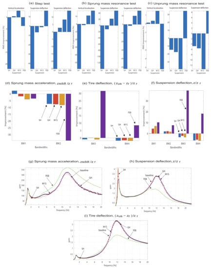
Figure 16.
Results from closed simulations for the comparison in a nonlinear QoV model considering a baseline suspension.
3.1.2. Closed Loop
The results in closed loop are presented for the normal QoV, the modified QoV (in-wheel electric motor) and the modified QoV (in-wheel electric motor) considering the residual vertical force provided by the electric motor in Figure 16, Figure 17 and Figure 18, respectively.
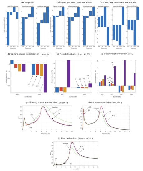
Figure 17.
Results from closed simulations for the comparison in a nonlinear modified QoV model considering a baseline suspension.
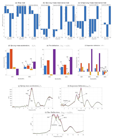
Figure 18.
Results from closed simulations for the comparison in a nonlinear modified QoV model considering a baseline suspension and the residual vertical force.
For the case of the MQoV, in the step test (Figure 17a), the M1S is the unique controller that enhances the comfort () which means that in comparison with an intermediate current value () the M1S enhances the damping action during compression. By the case of the sprung mass test (Figure 17b), the best performance in comfort is giving by the FEB controller (), followed by the M1S. The rest of controllers decreases the performance. In the frequency domain, the SH controller gives a minimum improvement () according to the IPSD (Figure 17d), and the pseudo-bode plot (Figure 17d), where it can be seen that the performance of the SH is similar to the baseline, which means that the baseline suspension is also a good option for improving comfort. According to the indexes discussed above, we can conclude that the SH enhances the comfort for the MQoV in closed loop considering as reference a baseline suspension. By the side of the road holding, in the step test (Figure 17a), FEB controller gives the highest improvement () followed by the M1S and GH controllers. For the unsprung mass test (Figure 17c), the best road holding performance () is also given by the FEB controller, the rest of controllers, decreases the performance in comparison with the baseline. By the side of the frequency domain, the FEB controller provides the best improvement () as well as the lowest gains in the bandwidths of interest, as it is shown in Figure 17i,e. The rest of the controllers gives almost the same performance than the baseline. According to the performance indexes, for the ModQoV, the best road holding improvement is given by the FEB controller in closed loop considering as reference a baseline suspension. The useful lifetime is improved by the FEB controller during the step, sprung and unsprung mass tests by , and , respectively. The same occurs in the frequency domain, where the FEB enhances the useful lifetime in a according to the IPSD, and minimizes the gains in the pseudo-bode plot. In the step and sprung mass test (Figure 17a,b) the FEB controller gives the biggest improvement followed by the M1S, while the rest of controllers decreases the performance. By the side of the unsprung mass test (Figure 17c), just the FEB controller is giving a useful lifetime improvement. The same occurs in the frequency domain, where the main improvement is giving by the FEB controller according to the Figure 17f,h and the rest of the controllers shows similar improvements in comparison with the baseline. That’s why the FEB controller guarantees the useful lifetime improvement for the MQoV in closed loop considering as reference a baseline suspension.
In the MQoVFV, comfort is improved in the step test (Figure 18a) by the SH controller in a followed by the GH controller, the rest of the controllers gives negative improvements. Besides, in the sprung mass test (Figure 18b), the comfort is enhanced by the FEB controller by . While the rest of controllers shows lower improvements than the baseline suspension. On the other hand, according to the IPSD (Figure 18a), the GH controller enhances the comfort by a followed by the FEB controller. While in the pseudo-bode plot (Figure 18a), the lower gains are given by the SH controller followed by the GH controller. According to the information described above, it can be said that the SH controller gives the highest comfort improvement for the MQoVFV in closed loop. By the side of the road holding, the SH controller enhances it by during the step test (Figure 18a) followed by the GH controller. The rest of the controllers show negative improvements. While in the unsprung mass (Figure 18c), the road holding is enhanced by the FEB controller by , also followed by the GH controller. In the frequency domain occurs almost the same, the FEB followed by the GH controller enhances the tire deflection by in accordance with the IPSD (Figure 18e) as well as gives the lowest gains in the pseudo-bode plot (Figure 18i). According to the information discussed above, the highest road holding improvement in the MQoVFV is given by the FEB controller in closed loop tests when compared against the baseline suspension. Finally, the useful lifetime is improved by the baseline in the step test (Figure 18a), followed by the GH and M1S controllers. While in the sprung mass and unsprung mass tests (Figure 18b,c), the FEB controller enhances the useful lifetime in a and , respectively. Where the rest of the controllers shows negative improvements. The same occurs in the frequency domain, where according to the IPSD (Figure 18f) and to the pseudo-bode plot (Figure 18h) gains, the FEB controller enhances the performance by . That’s why it can be stated that the FEB controller gives the higher useful lifetime improvement for the MQoVFV in closed loop, which means that suspension deflection has been decreased by the FEB controller.
From the PSB’s best cases shown in Figure 19, it can be seen that in comparison with the other QoVs, the MQoVFV is showing higher gains in the resonance frequencies for all the interest variables. Among all the QoV’s exists resonance frequencies displacements, but in the displacement for the MQoVFV seems to be a little bit higher. For the sprung mass acceleration in open and closed loop, the best performance improvement is given by the in open loop for the NQoV and for the MQoV and by the FEB controller in closed loop. While for the MQoVFV, the best improvement is given by the and by the GH controller for open and closed loop, respectively. For the rest of the interest variables, the best performance improvement is given by the same current and control strategy in all the QoV’s.
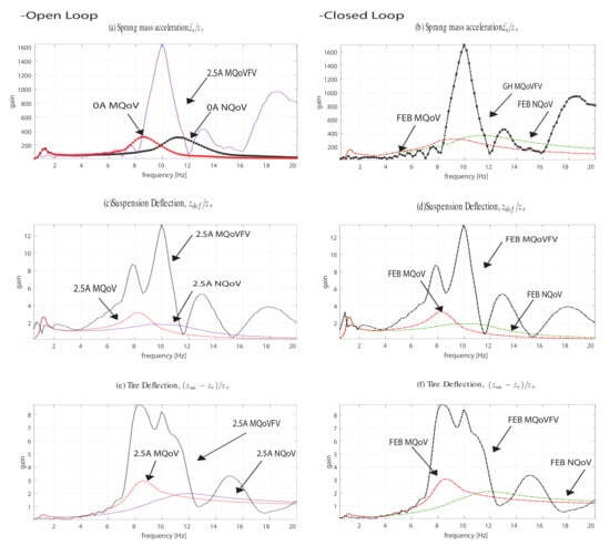
Figure 19.
Pseudo-Bode best cases for transfer functions in open and closed loop simulation considering a baseline suspension for the three QoVs.
3.2. Full Vehicle
For presenting the full vehicle results in a summarized way as in Figure 20, three interest variables (body acceleration, roll, and lateral acceleration) of those described in Section 2.9 are considered. The body acceleration from the BSST is employed to visualize the comfort performance. While for analyzing the road holding performance, the roll and the lateral acceleration are taken from the DLC and FSH tests, respectively.
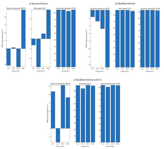
Figure 20.
Full vehicle results.
The results for the full vehicle simulations are shown in Figure 20. The comfort improvement in the normal vehicle according to the body acceleration (Figure 20a) is given by the FEB controller followed by the GH. For the modified vehicle, the highest comfort improvement is given by the baseline suspension in accordance with the body acceleration (Figure 20b). When the unbalanced vertical force is taken into account, the highest comfort improvement is given by the M1S controller. Followed by the SH (Figure 20c). The highest roll improvement () in the normal vehicle is given by the FEB controller and followed by the M1S in accordance with the results shown in Figure (Figure 20a). For the modified vehicle, the highest roll improvement () is given by the SH controller, followed by the M1S and GH controllers. While when the unbalanced vertical force is taken into account, the M1S gives the best improvement (), followed by the SH controller. By the side of the road holding, the SH, GH, and FEB controllers are giving the biggest improvement in the lateral acceleration. However, the best improvement is giving by the GH controller (). In the modified vehicle, the GH controller is also giving the best performance () and is closely followed by the M1S and SH controllers. When considering the unbalanced vertical force, the highest road holding improvement () is given by the M1S. And as can be seen, the rest of the controllers is almost giving the same results.
For the modified vehicle with and without the unbalanced vertical force occurs almost the same, the FEB and the M1S controllers (Figure 20e,h) give the best roll improvement. Finally the road holding improvement in the normal vehicle as well as in the modified vehicle without the unbalanced vertical force is given by the FEB controller, which produces the lower lateral acceleration magnitudes (Figure 20c,f). While for the modified vehicle with the unbalanced vertical force, the highest road holding improvement is given by the M1S closely followed by the GH controller (Figure 20i).
4. Conclusions
In this work, the use of semi-active suspension systems in in-wheel electric vehicles as a way for reducing vibrations due to the road profile and to the SR motor was explored considering the SR motor as a part of the unsprung mass and the unbalanced vertical force due to the SR motor. One of the main findings in this work, is that for improving the comfort when the unbalanced vertical force is considered, higher current values are required in comparison with the other QoV’s configurations. Likewise, the presence of the unbalanced vertical force seems to be giving higher gains in the frequency domain responses (pseudo-bode plots) for the interest variables. Where also a displacement of the resonance frequencies is visualized. From the full vehicle results, it can be said that for the normal vehicle, the FEB controller is guaranteeing the best improvement for comfort and road holding. While for the modified vehicle, the best comfort improvement is given by the baseline suspension. In road holding, all the controllers seems to be giving the same improvement. When the unbalanced vertical force is considered the SH and M1S controllers giving the best improvement for comfort and road holding objectives. As further work, a road profile identification is expected to be implemented for real-time switching between control strategies as a way for guaranteeing suspension systems adaptability to road conditions in EVs. As well, the use of semi-active suspension systems considering an extra mass due to the SR motor, where the rotor and the stator are considered as different masses and also when the whole SR motor is employed as an ADM might be explored.
Author Contributions
Conceptualization, M.A.-M. and J.-d.-J.L.-S.; Methodology, M.A.-M., J.-d.-J.L.-S.; Software, M.A.-M.; Validation, J.-d.-J.L.-S, J.-C.T.-M. and L.F.-H.; Investigation, M.A.-M.; Writing—original draft preparation, M.A.-M.; Writing—review and editing, M.A.-M., J.-d.-J.L.-S. and L.C.F.-H.; Supervision, J.-d.-J.L.-S., J.-C.T.-M. and R.M.-M.; Project administration, R.M.-M. and R.-A.R.-M.; Funding acquisition, R.M.-M. and R.-A.R.-M. These authors contributed equally to this work. All authors have read and agreed to the published version of the manuscript.
Funding
This research was funded by Tecnologico de Monterrey, School of Engineering and Sciences, Monterrey, NL, Mexico. And by Consejo Nacional de Ciencia y Tecnología (CONACYT).
Acknowledgments
First author is recipient of the excellence scholarship by Consejo Nacional de Ciencia y Tecnología (CONACYT) (CVU:930302) and Instituto Tecnológico de Estudio Superiores de Monterrey (A01328335) in the academic master’s program of manufacturing systems.
Conflicts of Interest
The authors declare no conflict of interest.
References
- Zhu, Y.; Zhao, C.; Zhang, J.; Gong, Z. Vibration Control for Electric Vehicles With In-Wheel Switched Reluctance Motor Drive System. IEEE Access 2020, 8, 7205–7216. [Google Scholar] [CrossRef]
- Nagaya, G.; Wakao, Y.; Abe, A. Development of an In-Wheel Drive With Advanced Dynamic-Damper Mechanism. JSAE Rev. 2003, 24, 477–481. [Google Scholar] [CrossRef]
- Ma, Y.; Deng, Z.; Xie, D. Control of the Active Suspension for In-Wheel Motor. J. Adv. Mech. Des. Syst. Manuf. 2013, 7, 535–543. [Google Scholar] [CrossRef]
- Wang, Y.; Li, Y.; Sun, W.; Yang, C.; Xu, G. FxLMS Method for Suppressing In-Wheel Switched Reluctance Motor Vertical Force Based on Vehicle Active Suspension System. J. Control Sci. Eng. 2014, 2014, 486140. [Google Scholar] [CrossRef]
- Shao, X. Active Suspension Control of Electric Vehicle with In-Wheel Motors. Ph.D. Thesis, School of Electrical, Computer and Telecommunications Engineering, University of Wollongong, Wollongong, Australia, 2018. [Google Scholar]
- Shao, X.; Naghdy, F.; Du, H. Reliable fuzzy H∞ control for active suspension of in-wheel motor driven electric vehicles with dynamic damping. Mech. Syst. Signal Process. 2017, 87, 365–383. [Google Scholar] [CrossRef]
- Liu, M.; Zhang, Y.; Huang, J.; Zhang, C. Optimization Control for Dynamic Vibration Absorbers and Active Suspensions of In-Wheel-Motor-driven Electric Vehicles. Proc. Inst. Mech. Eng. Part D J. Autom. Eng. 2020, 0954407020908667. [Google Scholar]
- Li, Z.; Zheng, L.; Ren, Y.; Li, Y.; Xiong, Z. Multi-objective Optimization of Active Suspension System in Electric Vehicle With In-Wheel-Motor Against The Negative Electromechanical Coupling Effects. Mech. Syst. Signal Process. 2019, 116, 545–565. [Google Scholar] [CrossRef]
- Dong, X.M.; Yu, M.; Liao, C.R.; Chen, W.M. Comparative Research on Semi-Active Control Strategies for Magneto-Rheological Suspension. Nonlinear Dyn. 2010, 59, 433–453. [Google Scholar] [CrossRef]
- Qin, Y.; Dong, M.; Langari, R.; Gu, L.; Guan, J. Adaptive Hybrid Control of Vehicle Semiactive Suspension Based on Road Profile Estimation. Shock Vib. 2015, 2015, 636739. [Google Scholar] [CrossRef]
- Song, C.; Zhou, Z.; Xie, S.; Hu, Y.; Zhang, J.; Wu, H. Fuzzy Control of a Semi-Active Multiple Degree-of-Freedom Vibration Isolation System. J. Vib. Control 2015, 21, 1608–1621. [Google Scholar] [CrossRef]
- Zhang, J.; Gao, R.; Zhao, Z.; Han, W. Fuzzy Logic Controller Based Genetic Algorithm for Semi-Active Suspension. J. Sci. Ind. Res. 2012, 71, 521–527. [Google Scholar]
- Félix-Herrán, L.C.; Mehdi, D.; Rodríguez-Ortiz, J.d.J.; Soto, R.; Ramírez-Mendoza, R. Hinfinite Control of a Suspension with a Magnetorheological Damper. Int. J. Control 2012, 85, 1026–1038. [Google Scholar] [CrossRef]
- Do, A.L.; Sename, O.; Dugard, L.; Savaresi, S.; Spelta, C.; Delvecchio, D. An Extension of Mixed Sky-hook and ADD to Magneto-Rheological Dampers. In Proceedings of the 4th IFAC Symposium on System, Structure and Control, Ancona, Italy, 15–17 September 2010. [Google Scholar]
- Hong, K.S.; Sohn, H.C.; Hedrick, J.K. Modified Skyhook Control of Semi-Active Suspensions: A New Model, Gain Scheduling, and Hardware-in-the-Loop Tuning. J. Dyn. Sys. Meas. Control 2002, 124, 158–167. [Google Scholar] [CrossRef]
- Liu, Y.; Zuo, L. Mixed Skyhook and Power-Driven-Damper: A New Low-Jerk Semi-Active Suspension Control Based on Power Flow Analysis. J. Dyn. Syst. Meas. Control 2016, 138, 081009. [Google Scholar] [CrossRef]
- Yerge, R.M.; Shendge, P.; Paighan, V.; Phadke, S. Design and Implementation of a Two Objective Active Suspension Using Hybrid Skyhook and Groundhook Strategy. In Proceedings of the 2017 2nd IEEE International Conference on Recent Trends in Electronics, Information & Communication Technology (RTEICT), Bangalore, India, 19–20 May 2017; pp. 968–972. [Google Scholar]
- Valášek, M.; Novak, M.; Šika, Z.; Vaculin, O. Extended Ground-Hook-New Concept of Semi-Active Control of Truck’s Suspension. Veh. Syst. Dyn. 1997, 27, 289–303. [Google Scholar] [CrossRef]
- Lozoya-Santos, J.D.J.; Morales-Menendez, R.; Ramírez Mendoza, R.A. Control of an Automotive Semi-Active Suspension. Math. Probl. Eng. 2012, 2012. [Google Scholar] [CrossRef]
- Jorge de J, L.S.; Morales-Menendez, R.; Ramirez-Mendoza, R.A.; Vivas-Lopez, C.A. Influence of MR damper Modeling on Vehicle Dynamics. Smart Mater. Struct. 2013, 22, 125031. [Google Scholar]
- Lozoya-Santos, J.d.J.; Cervantes-Muñoz, D.; Tudón-Martínez, J.C.; Ramirez-Mendoza, R.A. Off-road Motorbike Performance Analysis Using a Rear Semiactive EH Suspension. Shock Vib. 2015, 2015, 291089. [Google Scholar] [CrossRef]
- Poussot-Vassal, C. Commande Robuste LPV Multivariable de Chassis. Ph.D. Thesis, INP Grenoble, Grenoble, France, 2008. [Google Scholar]
- Lee, H.S.; Choi, S.B. Control and Response Characteristics of a Magneto-Rheological Fluid Damper for Passenger Vehicles. J. Intell. Mater. Syst. Struct. 2000, 11, 80–87. [Google Scholar] [CrossRef]
- Sohn, H.C.; Hong, K.S.; Hedrick, J.K. Semi-Active Control of the Macpherson Suspension System: Hardware-in-the-Loop Simulations. In Proceedings of the IEEE International Conference on Control Applications, Anchorage, AK, USA, 25–27 September 2000; pp. 982–987. [Google Scholar]
- Lozoya-Santos, J.D.J.; Morales-Menendez, R.; Ramirez-Mendoza, R.A. Evaluation of on–off Semi-Active Vehicle Suspension Systems by Using the Hardware-in-the-Loop Approach and the Software-in-the-Loop Approach. Proc. Inst. Mech. Eng. Part D J. Autom. Eng. 2015, 229, 52–69. [Google Scholar] [CrossRef]
- Rosli, R.; Mailah, M.; Priyandoko, G. Hardware-in-the-Loop Simulation for Active Force Control with Iterative Learning Applied to an Active Vehicle Suspension System. In Applied Mechanics and Materials; Trans. Tech. Publ.: Stafa-Zurich, Switzerland, 2014; Volume 465, pp. 801–805. [Google Scholar]
- Vos, R.; Besselink, I.; Nijmeijer, H. Influence of In-Wheel Motors on The Ride Comfort of Electric Vehicles. In Proceedings of the 10th International Symposium on Advanced Vehicle Control (AVEC10), Loughborough, UK, 22–26 August 2010; pp. 835–840. [Google Scholar]
- Lowe, M.; Tokuoka, S.; Trigg, T.; Gereffi, G. Lithium-Ion Batteries for Electric Vehicles; Duke University: Durham, NC, USA, 2010. [Google Scholar]
- Fraser, A. In-Wheel Electric Motors The Packaging and Integration Challenges. In Proceedings of the 10th International CTI Symposium, Novi, MI, USA, 15–18 May 2011; pp. 12–23. [Google Scholar]
- De Jesus Lozoya-Santos, J.; Sename, O.; Dugard, L.; Morales-Menéndez, R.; Ramirez-Mendoza, R. A LPV Quarter of Car with Semi-Active Suspension Model Including Dynamic Input Saturation. IFAC Proc. Vol. 2010, 43, 68–75. [Google Scholar] [CrossRef]
- Emura, J.; Kakizaki, S.; Yamaoka, F.; Nakamura, M. Development of the Semi-Active Suspension System Based on the Sky-Hook Damper Theory. SAE Trans. 1994, 103, 1110–1119. [Google Scholar]
- Savaresi, S.M.; Spelta, C. A Single-Sensor Control Strategy for Semi-Active Suspensions. IEEE Trans. Control Syst. Technol. 2009, 17, 143–152. [Google Scholar] [CrossRef]
- Sammier, D.; Sename, O.; Dugard, L. Skyhook and H∞ Control of Active Vehicle Suspensions: Some Practical Aspects. Veh. Syst. Dyn. 2003, 39, 279–308. [Google Scholar] [CrossRef]
- Boggs, C.; Borg, L.; Ostanek, J.; Ahmadian, M. Efficient Test Procedures For Characterizing MR Dampers. In Proceedings of the ASME 2006 International Mechanical Engineering Congress and Exposition, Chicago, IL, USA, 5–10 November 2006; pp. 173–178. [Google Scholar]
- Boggs, C.; Ahmadian, M.; Southward, S. Efficient Empirical Modelling of a High-Performance Shock Absorber For Vehicle Dynamics Studies. Veh. Syst. Dyn. 2010, 48, 481–505. [Google Scholar] [CrossRef]
- Fukushima, N.; Hidaka, K.; Iwata, K. Optimum Characteristics of Automotive Shock Absorbers Under Various Driving Conditions and Road Surfaces. Int. J. Veh. Des. 1983, 4, 463–472. [Google Scholar]
- Tudón-Martínez, J.C.; Lozoya-Santos, J.D.J.; Vivas, C.A.; Morales-Menendez, R.; Ramirez-Mendoza, R.A. Model-Free Controller for a Pick-up Semi-Active Suspension System. In Proceedings of the ASME 2012 International Mechanical Engineering Congress and Exposition, Houston, TX, USA, 9–15 November 2012; pp. 67–76. [Google Scholar]
- Jayahari, L.G.P. Correlation of Sinusoidal Sweep Test to Field Random Vibration. Master’s Thesis, Blekinge Institute of Technology, Karlskrona, Sweden, 2005. [Google Scholar]
- Forkenbrock, G.J.; Elsasser, D.; O’Harra, B. Nhtsa’s Light Vehicle Handling and Esc Effectiveness Research Program. In Proceedings of the International Technical Conference on the Enhanced Safety of Vehicles, Washington, DC, USA, 6–9 June 2005. [Google Scholar]
- Garrott, W.; Howe, J.; Forkenbrock, G. Experimental Examination of Selected Maneuvers That May Induce on-road Untripped, Light Vehicle Rollover. Accid. Reconstr. J. 2001, 12, 21–39. [Google Scholar]
- Nassirharand, A.; Taylor, J. Frequency-domain modeling of nonlinear multivariable systems. In Computer Aided Design in Control Systems 1988; Elsevier: Amsterdam, The Netherlands, 1989; pp. 301–305. [Google Scholar]
- Bastow, D.; Howard, G.; Whitehead, J.P. Car Suspension and Handling; SAE: Warrendale, PA, USA, 2004. [Google Scholar]
- Lu, J. A Frequency-Adaptive Multi-Objective Suspension Control Strategy. J. Dyn. Syst. Meas. Control 2004, 126, 700–707. [Google Scholar] [CrossRef]
- Delphi. Technical Report; Delphi. 2008. Available online: www.delphi.com (accessed on 20 June 2020).
- Gillespie, T.D. Fundamentals of Vehicle Dynamics; Society of Automotive Engineers: Warrendale, PA, USA, 1992; Volume 400. [Google Scholar]
- Els, P.S.; Theron, N.J.; Uys, P.E.; Thoresson, M.J. The Ride Comfort vs. Handling Compromise For Off-Road Vehicles. J. Terramech. 2007, 44, 303–317. [Google Scholar] [CrossRef]
- Ohsaku, S. Kinetic State Quantity Estimating Device and Method for Motor Vehicle. U.S. Patent 6,298,293, 31 May 2001. [Google Scholar]
- Uys, P.E.; Els, P.S.; Thoresson, M. Suspension Settings for Optimal Ride Comfort of Off-road Vehicles Travelling on Roads with Different Roughness and Speeds. J. Terramech. 2007, 44, 163–175. [Google Scholar] [CrossRef]
- Miller, L.R. Tuning Passive, Semi-Active, and Fully Active Suspension Systems. In Proceedings of the 27th IEEE Conference on Decision and Control, Austin, TX, USA, 7–9 December 1988; pp. 2047–2053. [Google Scholar]
- Ryu, J.; Moshchuk, N.K.; Chen, S.K. Vehicle State Estimation for Roll Control System. In Proceedings of the 2007 American Control Conference, New York, NY, USA, 9–13 July 2007; pp. 1618–1623. [Google Scholar]
© 2020 by the authors. Licensee MDPI, Basel, Switzerland. This article is an open access article distributed under the terms and conditions of the Creative Commons Attribution (CC BY) license (http://creativecommons.org/licenses/by/4.0/).