Article

A Deep Learning-Based Perception Algorithm Using 3D LiDAR for Autonomous Driving: Simultaneous Segmentation and Detection Network (SSADNet)

1
Department of Future Convergence Technology, Soonchunhyang University, Asan 31538, Korea
2
Department of Smart Automobile, Soonchunhyang University, Asan 31538, Korea
*
Author to whom correspondence should be addressed.
Appl. Sci. 2020, 10(13), 4486; https://doi.org/10.3390/app10134486
Submission received: 23 May 2020 / Revised: 13 June 2020 / Accepted: 23 June 2020 / Published: 29 June 2020
(This article belongs to the Special Issue Intelligent Transportation Systems: Beyond Intelligent Vehicles)

Abstract

:
In this paper, we propose a deep learning-based perception method in autonomous driving systems using a Light Detection and Ranging(LiDAR) point cloud data, which is called a simultaneous segmentation and detection network (SSADNet). SSADNet can be used to recognize both drivable areas and obstacles, which is necessary for autonomous driving. Unlike the previous methods, where separate networks were needed for segmentation and detection, SSADNet can perform segmentation and detection simultaneously based on a single neural network. The proposed method uses point cloud data obtained from a 3D LiDAR for network input to generate a top view image consisting of three channels of distance, height, and reflection intensity. The structure of the proposed network includes a branch for segmentation and a branch for detection as well as a bridge connecting the two parts. The KITTI dataset, which is often used for experiments on autonomous driving, was used for training. The experimental results show that segmentation and detection can be performed simultaneously for drivable areas and vehicles at a quick inference speed, which is appropriate for autonomous driving systems.

1. Introduction

An autonomous driving system involves recognizing the driving environment using sensors installed on a vehicle and deciding an optimal path for driving the vehicle autonomously. In general, autonomous driving systems consist of three modules for perception, decision, and control, and each module consists of algorithms corresponding to the role of a driver. The perception module recognizes the environment around the vehicle and evades static or dynamic obstacles using sensors installed on a vehicle while recognizing circumstances such as the location of a vehicle [1]. The decision module decides on driving strategies such as passing, turning, accelerating, or decelerating based on the recognized environment and determines the driving path to evade obstacles while driving on the target path. The control module controls the actuator to the targeted steering angle and vehicle speed according to the values determined by the judgment module [2]. The three modules of perception, decision, and control are closely related to each other in an autonomous driving system. In particular, the decision module and control module must have accurate perception to ensure safety and reliability [3]. Recently, there have been many studies on deep learning-based semantic segmentation and object detection using the data obtained from environment recognition sensors as input for the perception of an autonomous driving system for many-sided purposes in various environments [4,5,6].
Cameras and LiDAR are the most widely used sensors for recognizing the driving environment in an autonomous driving system. A camera is useful for recognizing the types of static and dynamic obstacles that a vehicle may encounter while driving. However, a camera is easily affected by environmental factors such as weather and intensity of illumination in which distortion may occur due to the characteristics of the camera lens. On the other hand, LiDAR is less affected by environmental factors than a camera, and it can obtain information on the environment around a vehicle through omnidirectional scanning without distortion. In general, moreover, LiDAR provides more accurate distance information than a camera and shows better environmental robustness than a camera. The most widely used deep learning-based perception methods for autonomous vehicles include semantic segmentation and object detection. First of all, semantic segmentation [7] is a process of classifying each pixel of an image into a distinct class label. Many sensors, such as camera or LiDAR, have been used for deep learning-based semantic segmentation [8,9]. Meanwhile, object detection [10] refers to classifying the class of each object in input images having multiple objects and even finding the location of those objects. To find the location, a bounding box is used in a regression analysis for prediction. Recently, research has been conducted on object detection using radar and camera [11,12].
A class corresponding to a certain bounding box can be identified through semantic segmentation, and the type of a specific object within a bounding box can be identified through object detection. Semantic segmentation and object detection are similar in the sense that the type and location of multiple objects can be identified. However, semantic segmentation has the advantage of being able to find specific areas within a space (such as drivable areas) by classifying them in a pixelwise manner, while object detection can find specific objects such as vehicles or pedestrians since the type of an object can be identified within a bounding box. Therefore, semantic segmentation and object detection use different methods depending on the target and purpose of recognition; thus, both processes are required for the perception in an autonomous driving system. In most studies, however, semantic segmentation and object detection have been considered as separate tasks. From the perspective of training, when networks are separately trained and inferred for segmentation and detection, time and resources are wasted in an autonomous driving system with limited computing resources. Namely, both semantic segmentation and object detection are very important roles for autonomous vehicle systems but need very large computational resources.
In many previous studies, semantic segmentation to which Fully Convolutional Network(FCN) [13] and U-Net [14] structures are applied has been performed based on images obtained using a camera, or object detection using Faster-RCNN [15], RetinaNet [16], or YOLOv3 [17] networks, with FCN modifying models trained for existing image classification in order to make them appropriate for the purpose of semantic segmentation. FCN is able to have spatial information by replacing a fully connected layer with a full-convolution layer, thus overcoming the limitations of a fully connected layer and influencing many subsequent semantic segmentation-related studies. U-Net uses the extended decoding method from FCN, U-Net proposed a semantic segmentation model in which encoders and decoders have symmetrical structures in the form of ‘U’ characters. Through the structure of connecting layers corresponding to each other in the encoder and decoder, more accurate localization is possible while maintaining semantic information. Faster-RCNN is a two-stage object detector that combines RPN, suggesting where the object might exist, and a detector that classifies the type of object and predicts the location of object. RetinaNet proposes a focal loss that gives small weights for well-classified classes and large weights for classes that are difficult to classify, so that all classes are well classified. YOLOv3 is a one-stage object detector that improves the existing YOLO and has better detection performance than other detectors. However, these image-based approaches have the limitations mentioned above, and only one semantic segmentation or object detection task is targeted. Furthermore, studies are being conducted on semantic segmentation such as RangeNet++ [18] and PointSeg [19] using a point cloud obtained by LiDAR and on object detection by PIXOR [20] and MV3D [21]. RangeNet++ is a method for performing rapid semantic segmentation by performing a spherical projection method for a 3D point cloud. PointSeg uses the light-weight network SqueezNet to improve speed and model accuracy. PIXOR performs object detection at high speed by reducing dimension by means of a top view projection of a 3D point cloud. MV3D is a method for performing object detection by fusing the top view projection, front view projection, and camera image of a 3D point cloud as input. However, these are also methods for either segmentation or detection, making them unsuitable for an autonomous driving system. Therefore, we introduce a SSADNet based on LiDAR that is stronger in terms of reliability than cameras for recognition, and integrates semantic segmentation and object detection into a single architecture.
In this paper, therefore, we introduce a method for performing segmentation and detection simultaneously for an autonomous driving system that uses LiDAR. This method can be applied to any type of environment without distortion to ensure the safety and reliability of the decisions and control modules that need to be processed in real world implementation using limited computing resources. The proposed network aims to be more favorable for real-world processing (which is necessary for an autonomous driving system) and the reasonable performance of segmentation and detection. While previous networks require more than one processor for each network, using more than one independent network to perform two functions, the proposed algorithm allows two functions to be performed simultaneously in one network structure, with fewer processors than conventional algorithms.
The results of the proposed network can be applied to lane-keeping, steering control, evading obstacles, collision prevention, speed control, and creating a driving path for autonomous driving and driving assistance. According to many recent studies, it is predicted that the development of autonomous driving technology and the spread of autonomous vehicles in the near future will lead to more advanced traffic safety standards, reduced environmental pollution, and improved social equality [22,23]. It is also expected that the annual number of self-driving cars will increase by 50 percent by 2030, global trade volume by 70 percent, and that the current number of cars will double to 1.2 billion by 2050 [23]. Accordingly, the purpose of this research is to enable safer and more reliable autonomous driving.
As input into the proposed network, a three-dimensional voxel-based point cloud obtained by a 3D LiDAR is first converted to a top view image of two-dimensional pixels. A pixel requires less storage space than a voxel and is more advantageous than a voxel in terms of the number of required operations [20]. The network for simultaneous segmentation and detection proposed in this study is trained using the point cloud top view image as input, and the training results can be used to obtain the segmentation and detection results. The network has a parallel structure of a segmentation branch and a detection branch. The segmentation branch transforms and expands the network (LoDNN) [24] for detecting the road, while the detection branch consists of a CNN that we designed. The segmentation and detection performance and the inference speed of the proposed network are investigated through training experiments.
This paper is structured as follows. Section 1 introduces the purpose and method of the research. In Section 2, the input data used for training and the configuration method are proposed. In addition, then, we explain the structure of the proposed network, and Section 3 introduces the experiments used for verifying the performance of the proposed network and the relevant results. Finally, we provide conclusions in Section 4 of this paper.

2. Simultaneous Segmentation and Detection Network (SSADNet)

2.1. Input Data Preprocessing

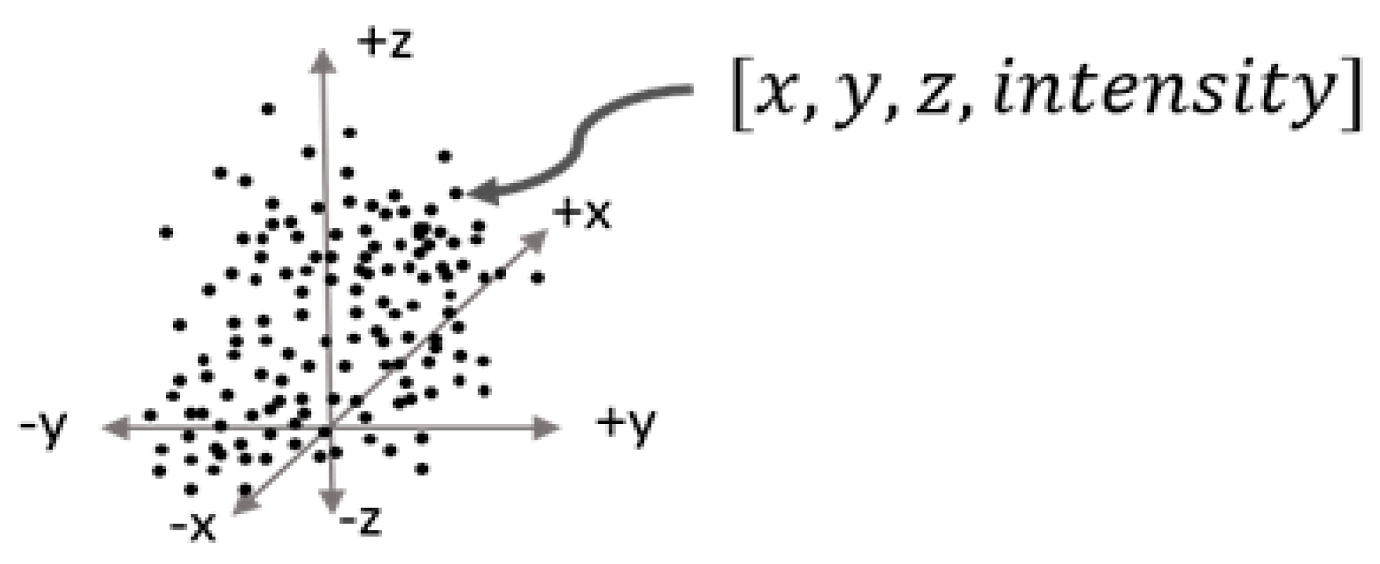
2.1.1. Point Cloud Data Representation

A point cloud is a set of points obtained using a 3D scanner such as LiDAR. As shown in Figure 1, each point includes information on the 3D location coordinates and the reflection intensity of the object surface. The coordinates of an object consist of the x-coordinate, y-coordinate, and z-coordinate on the 3D LiDAR coordinate system. The reflection intensity of the light (laser) is determined by the material color and the distance from a reflector.

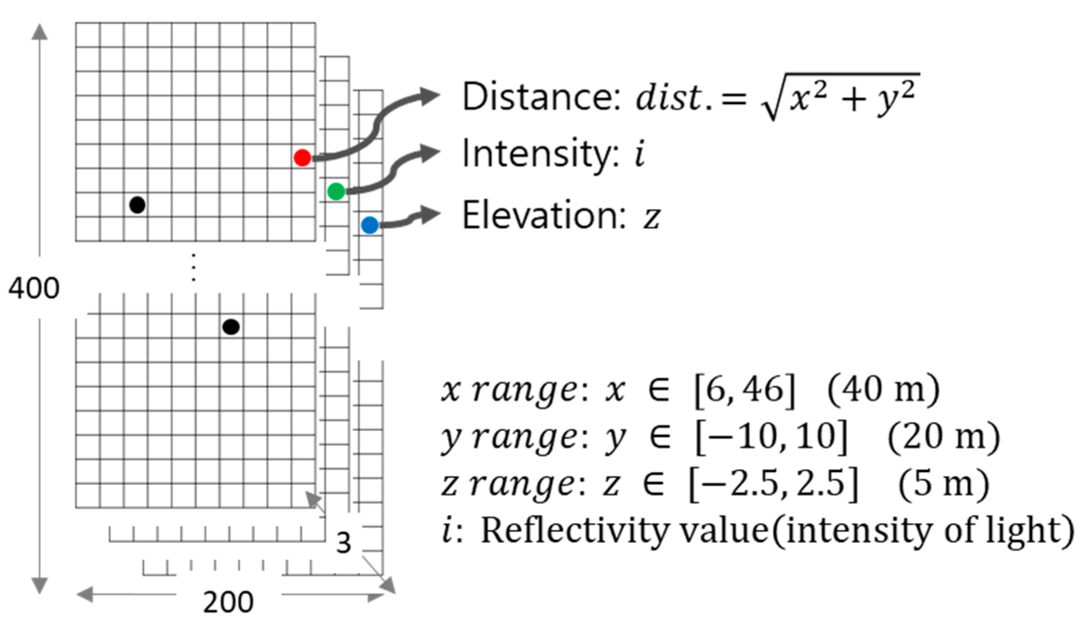
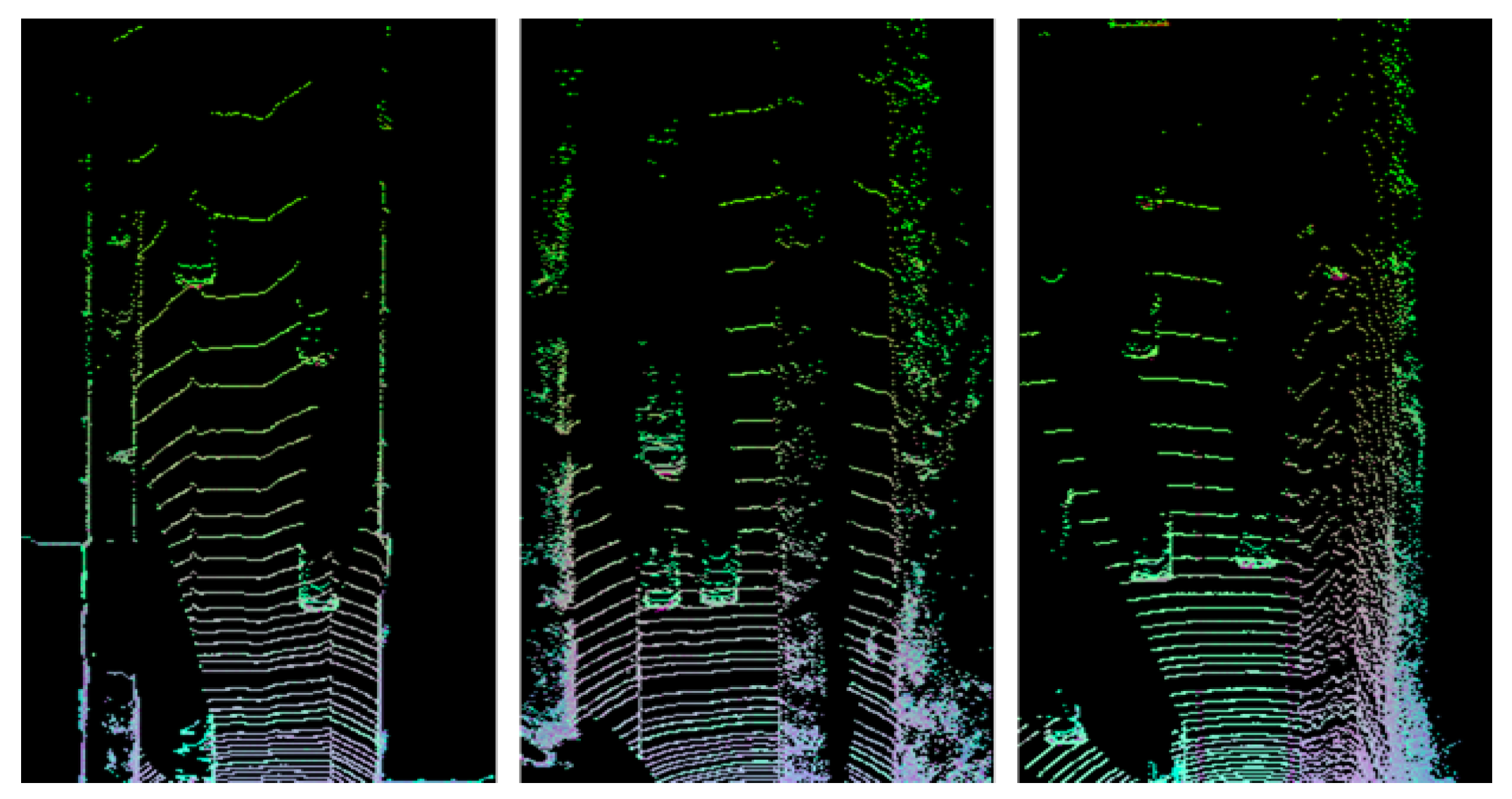
2.1.2. Point Cloud Top View Image

Generally, the input type of deep learning network for image processing consists of three channels. Each pixel of a normal three-channel image consists of information on the RGB color. However, since the type of data from LiDAR are different from the type of data in an image, we transformed the LiDAR data to image-type data. Each channel is configured using information from the point cloud data as shown in Figure 2.
Using the point cloud data, we created a new three-channel input for the proposed network. We generated three channel inputs using values of distance, reflection intensity, and height normalized within the range of [0, 255] for LiDAR point cloud data, and these are applied as input data for training the network.
The first channel of the point cloud top view image computes the distance information on the x-y plane of the 3D LiDAR coordinate system as in Equation (1). The second and third channels contain the reflection intensity and the height values (z-coordinate on the 3D LiDAR coordinate system) of the point cloud, respectively.
Distance = x 2 + y 2
The size of the point cloud top view image is associated with the ranges of x and y of the point cloud. The resolution of a 3D LiDAR sensor decreases as the distance increases; thus, the area of a point cloud in this study is limited for conversion to a top view image. The x-axis on the 3D LiDAR coordinate system ranged from 6 m to 46 m, while the y-axis ranged from −10 m to 10 m. In other words, the x-axis and the y-axis have a range of 40 m and 20 m, respectively. Furthermore, considering different heights of various vehicle types, the z-axis ranged from −2.5 m to 2.5 m for a 5 m range. Therefore, a top view image is generated only using a point cloud that is within the range of x∈ [6, 46], y∈ [−10, 10], and z∈ [−2.5, 2.5]. One pixel of the image represents a gap of 0.1 m. The generated point cloud top view image is 200 × 400 × 3 (width × height × channel). Figure 3 shows the top view image of the generated point cloud.

2.2. Simultaneous Segmentation and Detection Network (SSADNet)

In this section, we explain the structure and features of the network for the simultaneous segmentation and detection network (SSADNet) proposed in this paper. SSADNet trains the network using a point cloud top view image as input. It has the advantage of generating the results of segmentation and detection at the same time based on inference using the trained model.

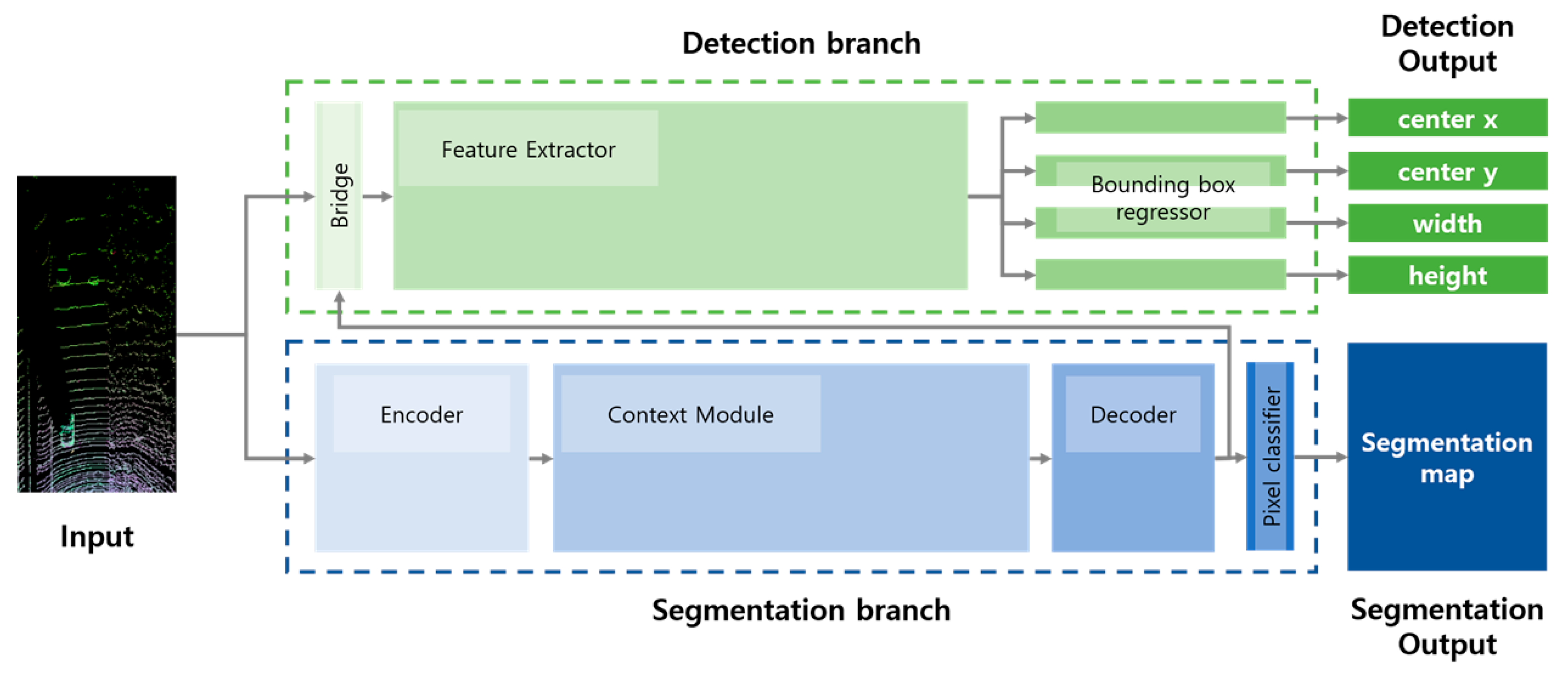
2.2.1. Architecture of SSADNet

The basic architecture of SSADNet is shown in Figure 4. SSADNet has two branched networks, i.e., the segmentation branch and detection branch, and a bridge part connecting the two branches. As opposed to other general CNN-based networks, SSADNet is applied with a fully convoluted layer structure [13] instead of a fully connected layer. A fully convoluted layer structure can have fewer parameters and a simpler model structure than a fully connected layer, thus allowing quick training and inference.
Moreover, SSADNet is applied with a dilated convolution filter [25] instead of a regular convolution filter to create a large receptive field with few parameters. Spatial dropout [26] was used in place of regular dropout [27,28]. Hence, the limitation of having dropouts with insignificant effects in a convolution layer was overcome, allowing us to maintain the regional features and prevent overfitting through generalization (which is the purpose of dropout). Moreover, an exponential linear unit (ELU) was applied as an activation function in which the slope did not reach 0 even with negative input, thus preventing the slope from plateauing. The ELU activation function is as shown in Equation (2).
f ( x ) = x   if   x > 0 f ( x ) = α ( e x 1 )   if   x 0

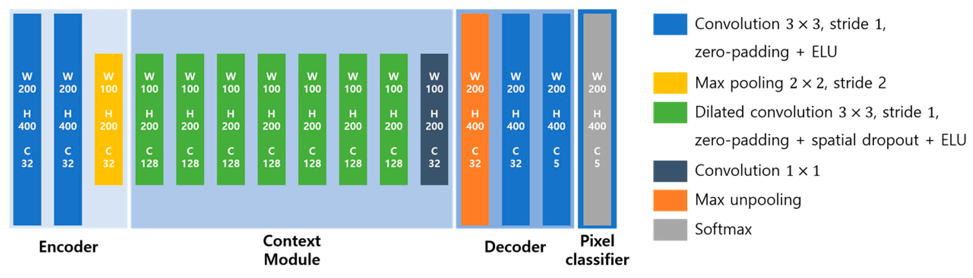
A. Segmentation Branch
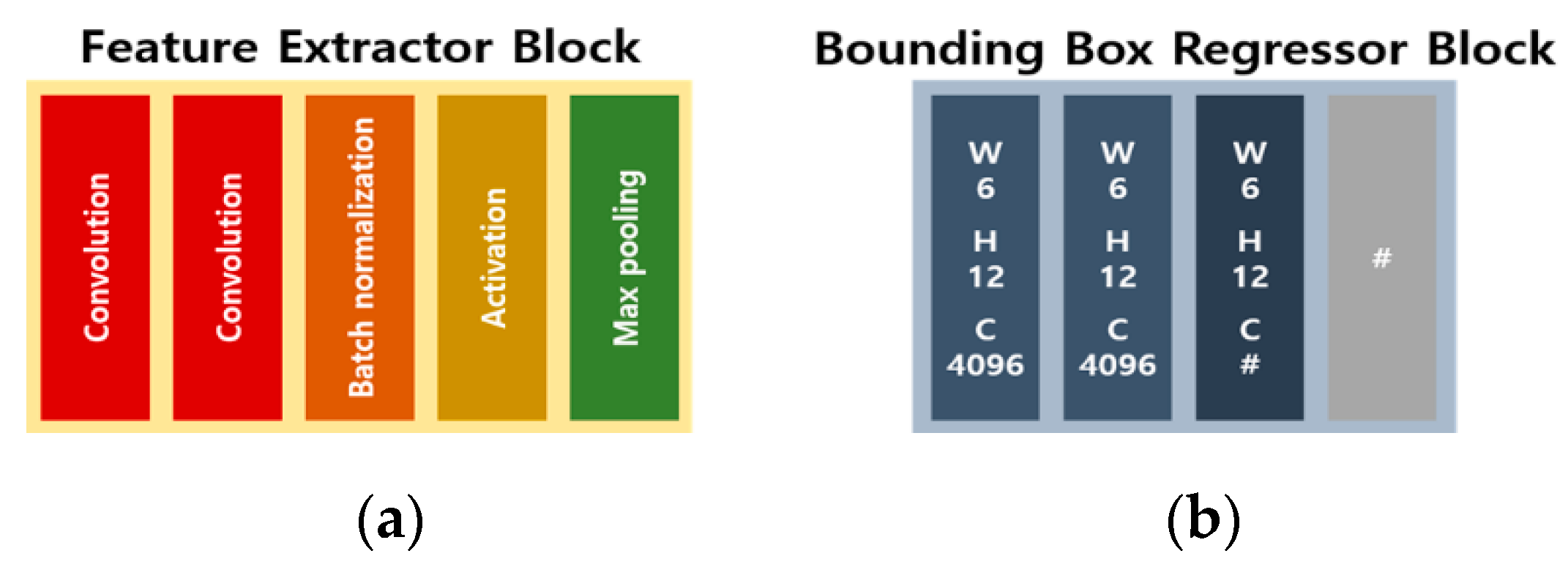
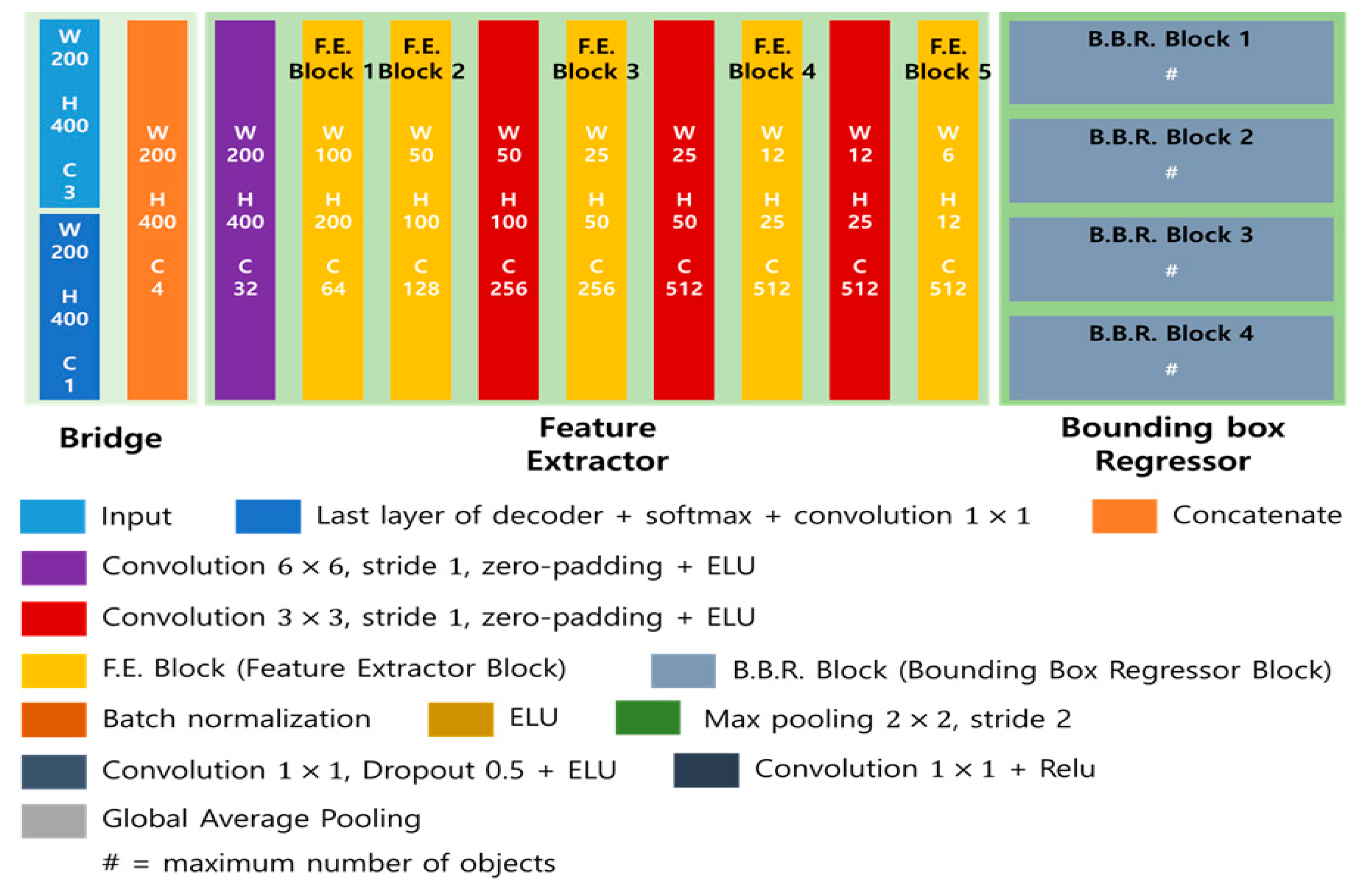
The segmentation branch in SSADNet for segmentation training and inference consists of four parts: the encoder–context module–decoder, and the fully convolutional layers for pixel classifiers. The structure of the segmentation branch was expanded and transformed to the LoDNN [24] structure so it could detect various types of vehicles and drivable road areas. Figure 4 shows the composition of a segmentation branch, and Figure 5 shows the detailed structure of a segmentation branch. The encoder in a segmentation branch compresses the input point cloud top view image, and extracts features. The context module was used to extract features from the compressed feature map to train it to decide which class each pixel belonged to. The decoder reconverted the compressed feature map to its original size and restored the location information. In the context module, a 3 × 3 dilated convolution filter having various receptive field sizes was applied using various dilation ratios (as shown in Table 1 and Figure 5) to extract information on drivable areas and the locations of vehicles. Furthermore, spatial dropout was used to maintain the extracted regional features while preventing overfitting. A pooling layer was applied several times, which simplified the structure of the encoder and decoder since larger receptive fields were obtained using a dilated convolution filter. The context module was used in between the simplified encoder–decoder structure to extract features. A softmax transfer function, which is a pixel classifier connected to the last layer, was used to perform classification.
Unlike other previous semantic segmentation networks based on fully convolutional networks, and comprising an encoder–decoder structure, our proposed segmentation branch of SSADNet applies a context module between the encoder and decoder. The dilated convolution filter is to expand the receptive field by adding zero-padding to the convolution filter, and we constructed the context module using a dilated convolution filter with various dilation rates. Therefore, the context module is able to play a role in extracting the feature with a dilated convolution filter with various receptive field and different sizes of receptive fields can be enabled to extract feature from objects of different sizes. This means that the encoder and the corresponding decoder can be simplified, because they can have a large receptive field by applying a dilated convolution filter so that the pooling does not require compression of the feature map. For point cloud top view images, it is more appropriate to extract features from high-resolution feature maps by dilated convolution than to compress feature maps through pooling, because transformed images become sparse data.
The structure of encoder before the context module is a 3 × 3 convolution filter with zero-padding of stride 1 and an ELU activation function twice in total, and 2 × 2 maxpooling with stride 2 for making a half size feature map. As shown in Table 1, the context module is designed with a 3 × 3 dilation convolution filter with increasing dilation rate and increasing reception field, spatial dropout, and ELU activation, and the last part is designed with a 1 × 1 convolution filter. The decoder corresponds to the reverse order of the encoder, restoring the reduced feature map from the encoder to its original size through max unpooling, 3 × 3 convolution filter and zero-padding of stride 1, and the ELU activation function repeats twice in total.

B. Detection Branch

A detection branch in SSADNet for detection training and inference has an FCN structure, including a bridge connecting the segmentation branch and the detection branch, a feature extractor, and bounding box regressor as shown in Figure 4. The bridge stacks the activation map obtained from the decoder of a segmentation branch in the direction of the input and channel. We expected this to suggest areas where the object being detected was located within the input image. The feature extractor performed extraction through convolution and pooling layers. The feature maps obtained from the feature extractor were placed in four bounding box regressors for predicting the x and y coordinates of a center point as well as the width and height of a bounding box. Each feature map was trained by updating parameters. The object class can be found from the class that corresponds to the coordinates of the center point of the bounding box in a segmentation map.
In SSADNet, the detection branch was connected to the segmentation branch to perform segmentation and detection simultaneously. The detection branch consists of the feature extractor and the bounding box regressor. Figure 6 shows (a) the feature extractor block (F.E. Block) for the feature extractor, and (b) the bounding box regressor block (B.B.R. Block) for the bounding box regressor, and Figure 7 shows the detailed structure of the detection branch. The feature extractor consists of five F.E. blocks. An F.E. block has a convolution filter layer which abstracts from simple features such as color, texture, edge, etc., to complex features which represent each class well, an activation layer, which gives non-linearity to the feature map in order to represent a complex model, and a pooling layer to reduce the feature map size or to prevent overfitting. In the detection branch, there are five F.E. Blocks (Feature Extractor) consisting of two 3 × 3 convolution filters with stride 1, batch normalization, ELU activation function, and 2 × 2 max pooling with stride 2, in order, and after each F.E. block except the first and last F.E. blocks, an additional 3 × 3 convolution filter with stride 1 is applied to extract the features.
After feature extraction from the feature extractor, the bounding box regressor branches out into four small branches, each re-regulating the width, height, and center point x and y coordinates, because the scales of the bounding box’s width, height, and center point x and y coordinate values are different. The bounding box regressor in the detection branch consists of four B.B.R. Blocks connected to the last F.E. Block. Each B.B.R. Block repeats the dropout and ELU to prevent over-fitting on the 1 × 1 convolution filter, after applying the 1 × 1 convolution filter and the ReLU activation and global average pooling [29].

2.2.2. Object Function

The overall loss function for optimizing the performance of backpropagation in the network proposed in this study is defined as shown in Equations (3)–(5). The overall loss function was calculated by separately multiplying the respective loss weight with a segmentation loss function and with a detection loss function and summing the resulting values. The loss function for segmentation, shown in Equation (4), is the cross-entropy loss between the ground truth and predicted results of the pixelwise classification performance [30]. The loss function for detection, shown in Equation (5), is the mean squared error of the bounding box label and predicted results regarding the x and y coordinates of a center point as well as the width and height of the bounding box. When training SSADNet, the detection loss was 10 times larger than the size of segmentation loss, which was set as a base. Hence, 0.1 times the loss weight of the detection loss was applied. In Table 2, the overall objective function consisted of a segmentation loss function and a detection loss function, and the notations of each item are shown. See Appendix A for more details.
L t o t = l w s e g × L s e g + l w d e t × L d e t
L s e g = 1 N × W × H n = 1 N w = 1 W h = 1 H ( y n , w , h t r u e × l o g ( y n , w , h p r e d ) )
L d e t = L c e n t e r _ x + L c e n t e r _ y + L w i d t h + L h e i g h t
L c e n t e r _ x ,     L c e n t e r _ y ,     L w i d t h ,     L h e i g h t = 1 N × n = 0 N 1 ( y n t r u e y n p r e d ) 2

3. Experiment Results and Discussion

3.1. Dataset

The KITTI dataset [31,32] provides sensor data of diverse weather conditions obtained on clear, rainy, or cloudy days and of various driving environments including downtown areas, outskirts, and highways using a camera, LiDAR, and GPS, along with annotation data for segmentation and detection. In this paper, we used the object detection database in the KITTI dataset. The KITTI object database consist of 7481 frames of labeled data and 7518 frames of unlabeled data, and the labels include object locations and pose information in each frame for object detection. To develop SSADNet, we used both label data and their LiDAR data.

3.1.1. Bounding Box Label

The left-top and right-bottom coordinates of a vehicle provided as a front view were converted to the top view coordinate system. The coordinates were then rotated using the yaw value. Then, the center point as well as the width and height of the bounding box (x, y) were calculated.

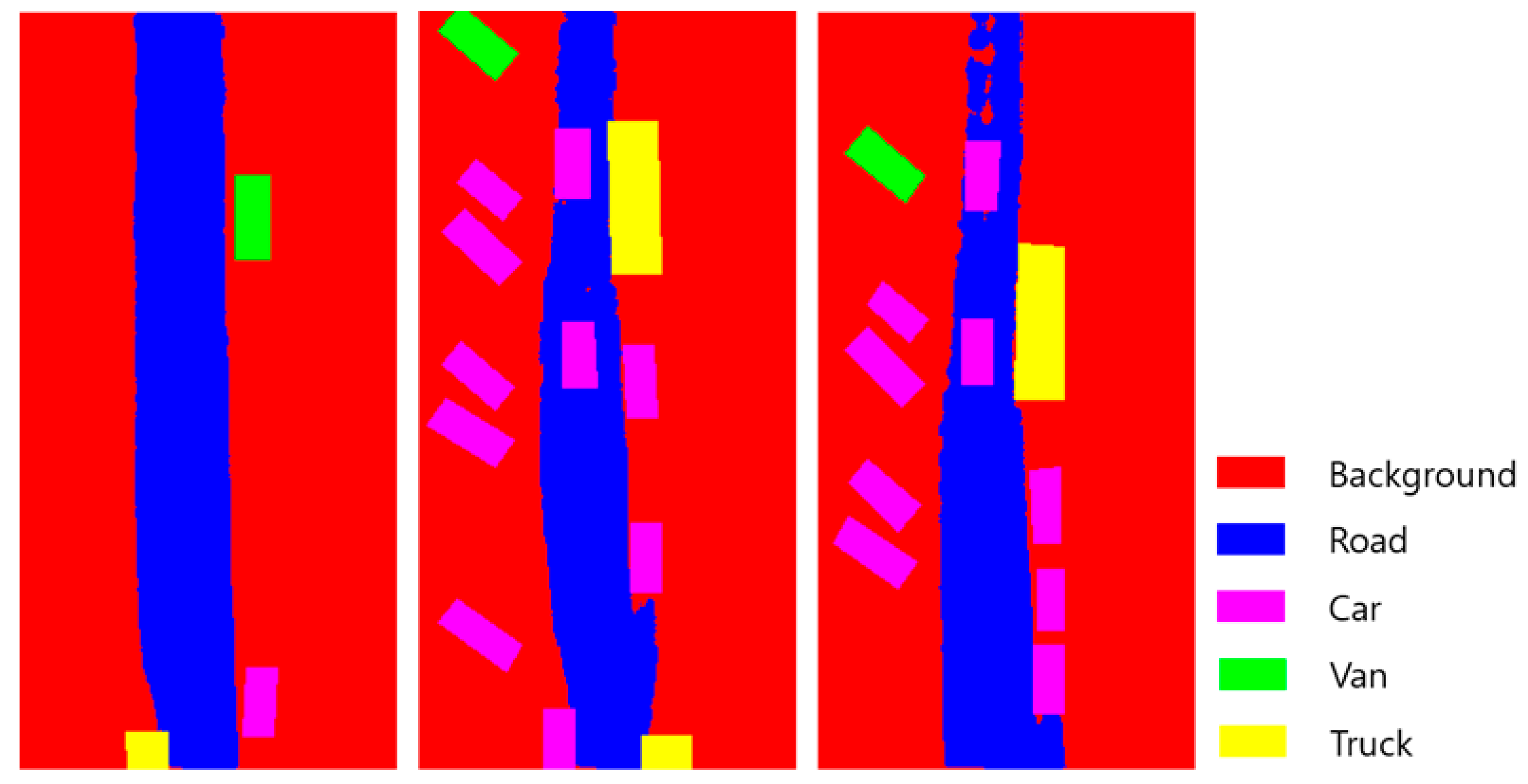
3.1.2. Segmentation Ground Truth

For the ground truth of a vehicle, the coordinates of a vehicle in a front view provided by the KITTI dataset were converted in the same way as the bounding box label. The predicted results of the network for detecting road regions (LoDNN) [24] were applied to the KITTI dataset in order to generate the ground truth of the drivable areas. There is a limitation in generating a ground truth that is identical to the actual object, because the resolution of LiDAR decreases as the distance increases. However, we verified that it was possible to generate ground truth in the experiment. In the generated segmentation answer shown in Figure 8, the blue color represents the ‘drivable region’, the magenta color represents a ‘car’, the green color represents a ‘van’, the yellow color represents a ‘truck’, and the red color represents ‘other regions (background)’.

3.2. Implementation Details

An Adam optimizer [33] with standard momentum was used for optimizing the objective function. The initial learning rate was 0.00001, and if loss was not reduced during 100 epochs for the validation set, the learning rate was reduced by 0.5 times. For the dataset, a total of 7481 pairs of point cloud top view images and answer data were divided at a ratio of 7:2:1 to form the training set (5237), validation set (1496), and test set (748). The distance, reflection intensity, height, and RGB values of the point cloud top view image used as input data were normalized in the range of [0, 1]. The x and y coordinates of the center point and the width and height of the bounding box in the answer data were also normalized in the range of [0, 1]. The size of the batch used for training was set to 8 to apply the maximum size allowed by the GPU according to the network structure or input method.
All codes for the experiment were written using Python 3. We implemented the deep learning model, and training, inference, and evaluation were performed using the Keras API and Tensorflow framework. The proposed network was trained using a NVIDIA GTX 1080Ti GPU having 11 GB of memory.

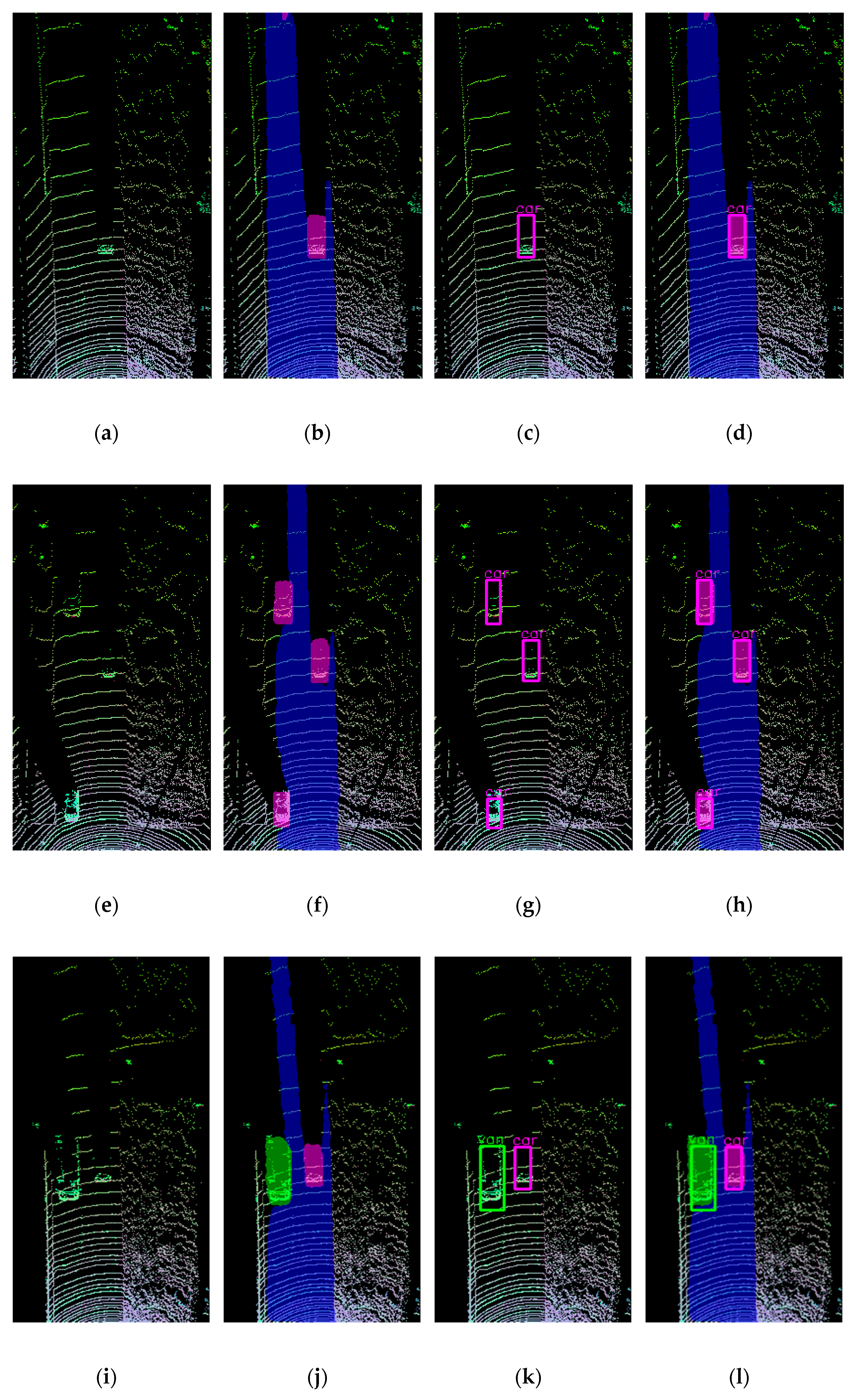
3.3. Results and Discussion

In this section, we introduce the indicators used for evaluating the performance of training. Among the performance indicators shown in Table 3, the segmentation performance was evaluated by pixelwise accuracy and average precision (AP). Moreover, to evaluate the detection performance, the critical value of mean intersection over union (mIoU) was set to 0.5 or greater (mIoU@0.5) and 0.7 or greater (mIoU@0.7). Then, the average of when the IoU of detected objects was equal to or greater than the critical value was calculated. The inference speed of each network was assessed in terms of frames per second (FPS). To assess the performance of the proposed network, we conducted a quantitative evaluation using performance indicators and a qualitative evaluation using visual images of segmentation and detection results.
Table 4 and Table 5 show the performance of the SSADNet. The segmentation performance had a pixelwise classification accuracy of 96.9%. The mAP was 96.9%, while the detection performance had a mIoU@0.5 of 70.5% and a mIoU@0.7 of 79.0%. The inference speed was 33 FPS. Figure 9 shows the visual results of SSADNet. From the left, each column in the figure represents an input image, segmentation result, detection result, and the results when segmentation and detection were performed simultaneously.
Table 6 and Table 7 show performance comparisons with other algorithms. Since our method was developed by converting 3D into 2D, we compared algorithms using frame image data which is same as LiDAR data.
In both detection and segmentation performance, the proposed method does not show much difference in performance from the other method. However, the advantage of SSADNet is that it provides sufficient computational speed with a single processor, while other algorithms need dual processors for deep learning to run segmentation and detection at the same time.

4. Conclusions

In this paper, we proposed a SSADNet that could simultaneously perform segmentation and detection of drivable regions and moving or non-moving vehicles in an autonomous driving system by generating a top view image using a point cloud obtained from 3D LiDAR.
The network was trained using the KITTI dataset, which is commonly used in research on autonomous driving systems. For network input, we generated a point cloud top view image having three channels of distance, reflection intensity, and height using the LiDAR point cloud. The segmentation performance of the proposed network had a pixelwise classification accuracy of 96.9%. The mAP was 96.9%, while the detection performance had a mIoU@0.5 of 70.5% and a mIoU@0.7 of 79.0%. The inference speed was 33 FPS. The experimental results can be applied for lane keeping, steering control, evading obstacles, collision prevention, speed control, and creating a driving path in autonomous driving or driving assistance.
The contributions of this paper are as follows: (1) we proposed a 3D point cloud-based detection and segmentation network using deep learning and (2) an algorithm that can perform two functions in one network structure simultaneously was proposed instead of a separate network structure that performs two functions. Namely, unlike previous algorithms need more than one processor for each network for detection and segmentation simultaneously, SSADNet can obtain detection and segmentation results for autonomous driving using a single network, so it can be done using a single processor.
However, this study has some limitations, in that the detection performance is poorer than the segmentation performance. SSADNet was not used for pre-trained models, so performance is limited when using the same number of training data, and after detection, reliable detection of obstacles is required through tracking algorithms such as the Kalman filter. Therefore, we will conduct further research (1) on improving the detection performance while maintaining the segmentation performance by enhancing the proposed network, (2) on increasing the speed to be more suitable for an autonomous driving system using pre-trained models, and (3) implementing the tracking algorithm in the time domain using Kalman filter, etc.

Author Contributions

Conceptualization, S.P.; methodology, Y.L. and S.P.; software, Y.L.; validation, Y.L.; formal analysis, Y.L. and S.P.; data curation, Y.L.; writing—original draft preparation, Y.L. and S.P.; writing—review and editing, Y.L. and S.P.; visualization, Y.L.; supervision, S.P.; project administration, S.P.; funding acquisition, S.P. All authors have read and agreed to the published version of the manuscript.

Funding

This works was supported by the National Research Foundation of Korea (NRF) grant funded by the Korea government (MSIP; Ministry of Science, ICT & Future Planning) (NRF-2017RIC1B5018101) and Soonchunhyang university 20160844.

Acknowledgments

The authors are very appreciate to journal editors and reviews.

Conflicts of Interest

The authors declare no conflict of interest.

Appendix A

To help readers understand, this section provides details of the performance metrics used to evaluate the performance of SSADNet.
First, we can evaluate segmentation performance using the IoU matrix in Figure A1a. The IoU can be calculated as the ratio of the overlapping pixel numbers between the real area and the predicted area. mIoU is obtained as the average value of all IoU of the segmented object for all test data. Precision in Equation (A3) can be obtained as a ratio of correctly predicted pixels (TP) that match the actual class with the predicted class among all pixels (TP + FP) predicted for one class, and mAP is obtained by averaging the Average Precision (AP) for all classes over the entire test set.
Figure A1. IoU (Intersection over Union): (a) for segmentation, (b) for detection.
Applsci 10 04486 g0a1
Detection evaluates performance using a ground truth bounding box and the predicted bounding box in Figure A1b. The IoU can be calculated as the ratio of the overlapping area between the real bounding box and the predicted bounding box. mIoU is obtained as the average value of the IoU for all images in the test set. Meanwhile, the precision of the detection is obtained as shown in (A3) by using TP for IoUs larger than the threshold set, and FP for IoUs smaller than the threshold. The mAP increases the recall from 0 to 1 (0, 0.1, 0.2, …, 1) and calculates the average of the corresponding precision when recall value is increasing over the entire class.
I o U = I n t e r s e c t i o n U n i o n
m I o U = t e s t   s e t I o U #   o f   t e s t   s e t
P r e c i s i o n = T P T P + F P
A P = A v e r a g e ( p r e c i s i o n ) m A P = A P #

References

  1. Yi, U.K.; Lee, J.W. Extraction of lane-related information and a real time image processing onboard system. Int. J. Automot. Technol. 2005, 6, 171–181. [Google Scholar]
  2. Lee, K.B.; Kim, Y.J.; Ahn, O.S.; Kim, Y.B. Lateral control of autonomous vehicle using Levenberg-Marquardt neural network algorithm. Int. J. Automot. Technol. 2002, 3, 71–77. [Google Scholar]
  3. Noh, S.-W.; Kim, T.-G.; Ko, N.Y.; Bae, Y.-C. Particle filter for correction of GPS location data of a mobile robot. J. Korea Inst. Electron. Commun. Sci. 2012, 7, 381–389. [Google Scholar]
  4. Wang, K.; Yan, F.; Zou, B.; Tang, L.; Yuan, Q.; Lv, C. Occlusion-free road segmentation leveraging semantics for autonomous vehicles. Sensors 2019, 19, 4711. [Google Scholar] [CrossRef] [Green Version]
  5. Sharma, S.; Ball, J.; Tang, B.; Carruth, D.W.; Doude, M.; Islam, M.A. Semantic segmentation with transfer learning for off-road autonomous driving. Sensors 2019, 19, 2577. [Google Scholar] [CrossRef] [Green Version]
  6. Vaquero, V.; Repiso, E.; Sanfeliu, A. Robust and real-time detection and tracking of moving objects with minimum 2D LiDAR information to advance autonomous cargo handling in ports. Sensors 2018, 19, 107. [Google Scholar] [CrossRef] [Green Version]
  7. Garcia-Garcia, A.; Orts-Escolano, S.; Oprea, S.; Villena-Martínez, V.; Garcia-Rodriguez, J. A Review on Deep Learning Techniques Applied to Semantic Segmentation. arXiv 2017, arXiv:1704.06857. [Google Scholar]
  8. Zou, N.; Xiang, Z.; Chen, Y.; Chen, S.; Qiao, C. Chen simultaneous semantic segmentation and depth completion with constraint of boundary. Sensors 2020, 20, 635. [Google Scholar] [CrossRef] [Green Version]
  9. Cai, G.; Jiang, Z.; Wang, Z.; Huang, S.; Chen, K.; Ge, X.; Wu, Y. Spatial aggregation net: Point cloud semantic segmentation based on multi-directional convolution. Sensors 2019, 19, 4329. [Google Scholar] [CrossRef] [Green Version]
  10. Zhao, Z.-Q.; Zheng, P.; Xu, S.-T.; Wu, X. Object detection with deep learning: A review. IEEE Trans. Neural Netw. Learn. Syst. 2019, 30, 3212–3232. [Google Scholar] [CrossRef] [Green Version]
  11. Chang, S.; Zhang, Y.; Zhao, X.; Huang, S.; Feng, Z.; Wei, Z.; Zhang, F. Spatial attention fusion for obstacle detection using MmWave radar and vision sensor. Sensors 2020, 20, 956. [Google Scholar] [CrossRef] [Green Version]
  12. Kuang, H.; Wang, B.; An, J.; Zhang, M.; Zhang, Z. Voxel-FPN: Multi-scale voxel feature aggregation for 3D object detection from LIDAR point clouds. Sensors 2020, 20, 704. [Google Scholar] [CrossRef] [PubMed] [Green Version]
  13. Long, J.; Shelhamer, E.; Darrell, T. Fully convolutional networks for semantic segmentation. arXiv 2015, arXiv:1411.4038. [Google Scholar]
  14. Ronneberger, O.; Fischer, P.; Brox, T. U-Net: Convolutional networks for biomedical image segmentation. In Intelligent Tutoring Systems; Springer Science and Business Media LLC: Berlin, Germany, 2015; Volume 9351, pp. 234–241. [Google Scholar]
  15. Ren, S.; He, K.; Girshick, R.; Sun, J. Faster R-CNN: Towards real-time object detection with region proposal networks. Adv. Neural Inf. Process. Syst. 2015, 91–99. [Google Scholar] [CrossRef] [PubMed] [Green Version]
  16. Lin, T.-Y.; Goyal, P.; Girshick, R.; He, K.; Dollar, P. Focal loss for dense object detection. In Proceedings of the IEEE International Conference on Computer Vision (ICCV), Venice, Italy, 22–29 October 2017; pp. 2999–3007. [Google Scholar]
  17. Redmon, J.; Farhadi, A. YOLOv3: An incremental improvement. arXiv 2018, arXiv:1804.02767. [Google Scholar]
  18. Milioto, A.; Vizzo, I.; Behley, J.; Stachniss, C. RangeNet ++: Fast and Accurate LiDAR Semantic Segmentation. In Proceedings of the IEEE/RSJ International Conference on Intelligent Robots and Systems (IROS), Venetian, Macao, 3–8 November 2019; pp. 4213–4220. [Google Scholar]
  19. Wang, Y.; Shi, T.; Yun, P.; Tai, L.; Liu, M. PointSeg: Real-time semantic segmentation based on 3D LiDAR point cloud. arXiv 2018, arXiv:1807.06288. [Google Scholar]
  20. Yang, B.; Luo, W.; Urtasun, R. PIXOR: Real-time 3D object detection from point clouds. In Proceedings of the IEEE/CVF Conference on Computer Vision and Pattern Recognition, Salt Lake City, UT, USA, 18–22 June 2018; pp. 7652–7660. [Google Scholar]
  21. Chen, X.; Ma, H.; Wan, J.; Li, B.; Xia, T. Multi-view 3D object detection network for autonomous driving. In Proceedings of the IEEE Conference on Computer Vision and Pattern Recognition (CVPR), Honolulu, HI, USA, 21–26 July 2017; pp. 6526–6534. [Google Scholar]
  22. Fabio, A.; Pau, G.; Collotta, M. A survey on driverless vehicles: From their diffusion to security. J. Internet Serv. Inf. Secur. 2018, 8, 1–19. [Google Scholar]
  23. Arena, F.; Ticali, D. The development of autonomous driving vehicles in tomorrow’s smart cities mobility. AIP Conf. Proc. 2018, 2040, 140007. [Google Scholar] [CrossRef]
  24. Caltagirone, L.; Scheidegger, S.; Svensson, L.; Wahde, M. Fast LIDAR-based road detection using fully convolutional neural networks. IEEE Intell. Veh. Symp. 2017, 1019–1024. [Google Scholar] [CrossRef] [Green Version]
  25. Fisher, Y.; Koltun, V. Multi-scale context aggregation by dilated convolutions. arXiv 2015, arXiv:1511.07122. [Google Scholar]
  26. Tompson, J.; Goroshin, R.; Jain, A.; LeCun, Y.; Bregler, C. Efficient object localization using convolutional networks. arXiv 2015, arXiv:1411.4280. [Google Scholar]
  27. Hinton, G.E.; Srivastava, N.; Krizhevsky, A.; Sutskever, I.; Salakhutdinov, R.R. Improving neural networks by preventing co-adaptation of feature detectors. arXiv 2012, arXiv:1207.0580. [Google Scholar]
  28. Nitish, S.; Hinton, G.; Krizhevsky, A.; Sutskever, I.; Salakhutdinov, R. Dropout: A simple way to prevent neural networks from overfitting. J. Mach. Learn. Res. 2014, 15, 1929–1958. [Google Scholar]
  29. Min, L.; Chen, Q.; Yan, S. Network in network. arXiv 2013, arXiv:1312.4400. [Google Scholar]
  30. De Boer, P.-T.; Kroese, D.P.; Mannor, S.; Rubinstein, R.Y. A tutorial on the cross-entropy method. Ann. Oper. Res. 2005, 134, 19–67. [Google Scholar] [CrossRef]
  31. Geiger, A.; Lenz, P.; Stiller, C.; Urtasun, R. Vision meets robotics: The KITTI dataset. Int. J. Robot. Res. 2013, 32, 1231–1237. [Google Scholar] [CrossRef] [Green Version]
  32. Geiger, A.; Lenz, P.; Urtasun, R. Are we ready for autonomous driving? The KITTI vision benchmark suite. In Proceedings of the IEEE Conference on Computer Vision and Pattern Recognition, Providence, RI, USA, 16–21 June 2012; pp. 3354–3361. [Google Scholar]
  33. Kingma, D.; Ba, J. Adam: A method for stochastic optimization. arXiv 2014, arXiv:1412.6980. [Google Scholar]
Figure 1. The configuration of a point cloud.
Applsci 10 04486 g001
Figure 2. The configuration of point cloud top view image.
Applsci 10 04486 g002
Figure 3. An example of a point cloud top view image created.
Applsci 10 04486 g003
Figure 4. Architecture of Simultaneous Segmentation and Detection Network.
Applsci 10 04486 g004
Figure 5. Detailed structure of segmentation branch.
Applsci 10 04486 g005
Figure 6. Components of the detection branch: (a) feature extractor block, (b) boundary box regressor block.
Applsci 10 04486 g006
Figure 7. Detailed structure of the detection branch.
Applsci 10 04486 g007
Figure 8. An example of ground truth for segmentation.
Applsci 10 04486 g008
Figure 9. Qualitative results of SSADNet: (a,e,f) input image, (b,f,j) segmentation result, (c,g,k) detection result, (d,h,l) results that confirm segmentation and detection at the same time.
Applsci 10 04486 g009
Table 1. Context module of segmentation branch.
Context ModuleDilation Rate (Width, Height)Receptive Field
1(1, 1)3 × 3
2(1, 2)5 × 7
3(2, 4)9 ×15
4(4, 8)17 × 31
5(8, 16)33 × 63
6(16, 32)65 × 127
7(32, 64)129 × 255
8-129 × 255
Table 2. Notation related to loss function.
L t o t Total Loss
L s e g Segmentation loss (Cross-entropy)
L d e t Detection loss
L c e n t e r _ x Loss about center x coordinate of bounding box (MSE)
L c e n t e r _ y Loss about center y coordinate of bounding box (MSE)
L w i d t h Loss about width coordinate of bounding box (MSE)
L h e i g h t Loss about height coordinate of bounding box (MSE)
l w s e g Segmentation loss weight (=1.0)
l w d e t Detection loss weight (=0.1)
N Batch size
W Width of the Segmentation map
H Height of the Segmentation map
Table 3. Performance metrics.
mAPWeighted Average of the Number of Data Belonging to the Class for the Precision of Each Class
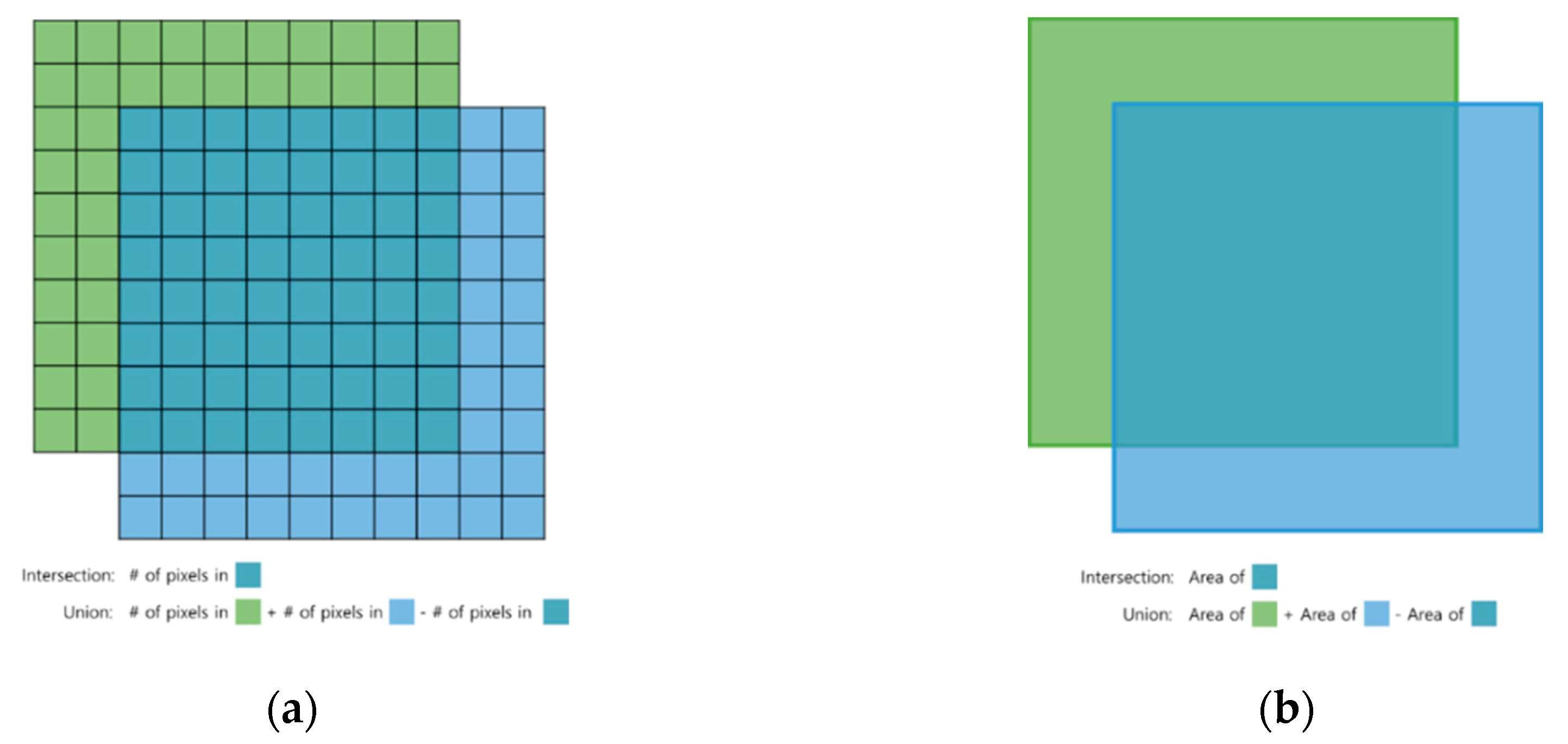
mIoUAverage of the ratio of overlapping areas to the sum of the real and predicted areas in the bounding box
FPSThe number of inference frames per second
Table 4. Quantitative performance of SSADNet segmentation.
ACC [%]mAP [%]mIoU [%]
96.9%96.9%83.57%
Table 5. Quantitative performance of SSADNet detection.
mAP50 [%]mIoU [%]
@0.5@0.7
85.02%70.48%79.03%
Table 6. Segmentation performance comparison.
MethodmIoU [%]
FCN-VGG16 [13]94.14%
LoDNN [24]85.68%
SSADNet (Proposed)83.57%
Table 7. Detection performance comparison.
MethodmAP50 [%]mIoU [%]
RetinaNet-ResNet50 [16]79.07%81.36%
YOLO v3 [17]77.78%75.74%
SSADNet (Proposed)85.02%70.48%

