1. Introduction
Advancements in computing power have allowed the development and implementation of more complex systems in vehicle development. The automotive industry has taken advantage of these advancements by creating and continuously improving advanced driver-assistance systems, such as automatic parking systems, road-assisted driving, and sometimes fully autonomous driving (AD) capacity [
1]. Urban, commercial, and industrial vehicles have been enhanced with these systems and are commonly known as Automated Guided Vehicles (AGV). Many automotive manufacturers have self-driving car development programs, including Tesla and Toyota. Additionally, other companies, such as Uber and Waymo, focus on the Transport as a Service (TaaS) industry. Finally, automated vehicles are also being employed inside warehouses or factories to automate distribution and optimize processes—e.g., Amazon [
2,
3].
There is still a long way to go before seeing this technology incorporated into all industries and transport services. The task of controlling a vehicle is not an easy one; it is a task that sometimes even the human being himself finds complicated to perform. The developed prototypes of self-driving car systems are required to fit industry and academic standards in terms of performance, safety, and trust [
2,
3]. The stand-alone navigation problem seemed to be solved after the Defense Advanced Research Projects Agency (DARPA) Grand and Urban Challenge [
4], however new problems popped up. They generated interest in the following research topics: data management, adaptive mobility, cooperative planning, validation, and evaluation. Data uncertainty and reliability represent the biggest challenges for data management. Without reliable data, the representation and modelling of the environment are at stake [
5]. The topic of adaptive mobility relates to the introduction of self-driving cars to conventional environments.
Therefore, the automation of the process is not simple. It is important to continue developing research in this area to improve upon the current technology surrounding autonomous vehicles, from the development of better sensors at a lower cost to the improvement of navigation algorithms with more advantageous designs, leading to the generation of more significant low-cost vehicular platforms.
This paper presents the results obtained from the navigation automation of a modular vehicular platform, intending to generate a low-cost modular AGV. Considering the minimum instrumentation necessary in addition to the algorithms needed to achieve such automation, this work integrates several of the most popular software and hardware tools used nowadays. The Robot Operating System (ROS) was used as an integrating software for the different instrumentation modules and sensors that allow controlling the vehicle; Behavioral Cloning (BC), an end-to-end algorithm, was used because of its ability to replicate human behavior when navigating the vehicle through an established route.
Numerous acronyms are frequently used in this work, which can be seen in
Appendix A.
This paper is organized as follows: The background overview section describes the related work and state-of-the-art developments in the field and compares them to the modular vehicle platform presented. The research approach presents the methodology used to develop the solution. The proposed system segment contains a thorough description of how the vehicle was instrumented, the minimum systems required to achieve Society of Automotive Engineers (SAE) Level 1 automation, and the test track. The development section reports how the stages in which the instrumentation, data acquisition, algorithm development, training, testing, and validation modules were developed over four weeks. The results segment presents the achievements of the AGV along with its performance metrics. The conclusion analyzes the problems faced and how they were solved along with the contributions of this work to areas of growth. Additionally, possible system upgrades are stated in the future work section.
2. Background Overview
The development of technologies that automate driving in the last decade has structured specific definitions and methodologies that allow the effective implementation of vehicles with the capacity to navigate over complex environments. These definitions and methodologies are the basis of the current development of autonomous vehicles, and it is the same basis used for the development of the solution presented in this work. These concepts are levels of driving automation, approaches to achieving navigation, and learning methods for navigation.
2.1. Levels of Driving Automation
Since 2014, the Society of Automotive Engineers (SAE) has published yearly the “SAE J3016 Levels of Driving Automation”, which defines six levels of automation ranging from 0, no automation, to 5, full vehicle autonomy [
6,
7,
8].
Table 1 briefly summarizes it.
2.2. Navigation Approaches
By defining the levels of driving automation, it is possible to know the scope and limitations that a navigation system must have when driving the vehicle. The generation of navigation systems for AVs has been achieved in recent years through various approaches.
Two main scopes aim to solve the navigation problem:
Traditional approach: It focuses on the individual and specialized tasks for perception, navigation, control, and actuation. The environment and the ego vehicle are modeled with the gathered data. Thus, for highly dynamic environments this approach is limited by the computing power, model complexity, and sensor quality. Robotic systems have used this modular solution for many years. Its complexity tends to be directly proportional to the model’s accuracy [
2,
3,
9].
End-to-end approach (E2E): This scope allows users to generate a direct correlation of the input data of a system with certain output data through the use of Deep Learning (DL). Artificial intelligence has been a breakthrough for AGVs. Machine learning (ML) serves to generate intelligent perception and control systems for robot navigation. Deep Learning (DL) is a state-of-the-art technique for creating models that resemble human behavior and decision-making [
10,
11,
12,
13,
14].
DL is trained with positive and negative examples using Deep Neural Networks (DNN). There are several types of architectures to choose from, including Convolution or Deconvolution layers, Recurrence or Memory layers, and Fully Connected Neurons, as well as Encoding or Decoding layers. These layers form popular architectures, such as Convolutional Neural Networks (CNN), Recurrent Neural Networks (RNN), Long-Short Term Memories (LSTM), and Fully Convolutional Networks (FCN), among others. Specific architectures have been generated by companies or development groups, such as LeNet, GoogLeNet, VGG, ResNet, Inception, and others [
15,
16]. The performance of each type of network will strongly depend on the data with which it is trained.
Data comes mostly from the ego vehicle’s front view, along with little processed data [
17,
18]. Outputs are usually referenced values to be given to closed-loop controllers for the steering, speed and braking systems [
14]. Among all the DNN, convolutional neural networks (CNN) have proven to be the most efficient ones for this type of task [
19]. Their inner layers extract and filter the information with which it is trained. CNNs correlate input images to control and actuate the variables of the AGV. Thus, the training process efficiency is increased. Only a few thousand data points are required to achieve acceptable accuracy [
20,
21,
22].
2.3. Learning Methods
Taking into account the scope using neural networks, different learning algorithms have achieved an effective navigation system for AGVs in simulated and real environments. Each algorithm has its advantages and disadvantages in different types of development environments. The two learning algorithms for this kind of neural networks are:
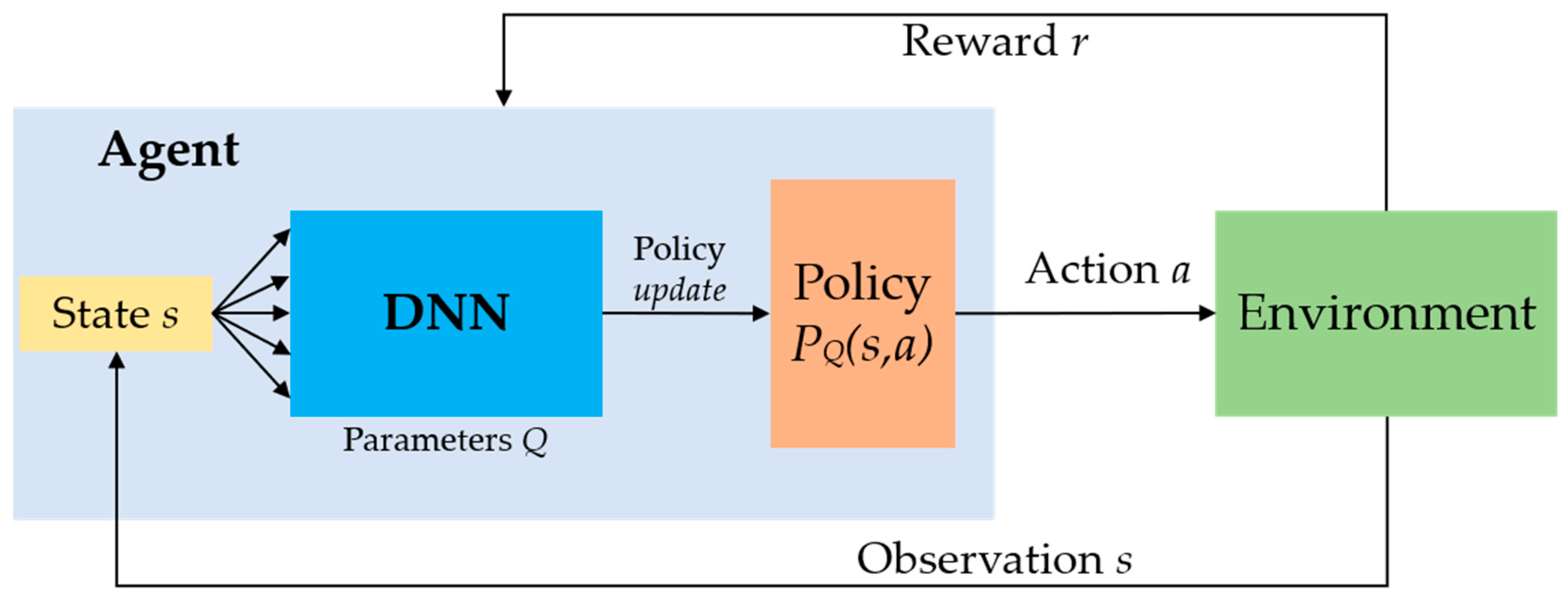
Deep Reinforcement Learning (DRL): This method optimizes a cost function by maximizing a reward or minimizing penalties, depending on which parameters are specified by the user. For example, a reward in an E2E approach regarding autonomous navigation could be to grant positive points if the platform remains inside a delimited lane mark and a negative point if it were to drive outside this area. Regarding this example, the cost function is composed of a set of rules of expected outcomes. A set of discrete randomized actions are tested in each scenario [
13]. The DNN will try iteratively to optimize the robot’s navigation within a lane [
23,
24,
25], merging [
24,
26], or exploring unknown environments [
27,
28]. The algorithm is described in
Figure 1.
A mapping algorithm would need to be implemented to delimit the lane marks that feed the image to the DNN and establish the reward rules and parameters. Not to mention that it is an iterative method, which means that the training of the DNN would need to happen as the platform drives itself in the chosen area. This is a risky approach, since no training has been carried out in the first iteration, so the platform would be driving itself around the area at the same time as it trains itself with the rewards and the penalties. This training is usually developed in big areas, or simulated as a first approach and then taken to the real world. This is dangerous, as in the first iterations the platform is going to drive outside the lane; it will break and accelerate very slowly or quickly. It can hurt somebody or even damage its own structure in the training process.
For this work, a safe area was chosen to acquire training data. No simulator was used. For that reason, DRL was not the approach used for the development of this work.
Behavioral Cloning/Imitation Learning (BC/IL): These algorithms are applications of supervised learning. They are iterative processes in which a network modifies its weights when given a set of inputs with its corresponding outputs. The training and validation datasets contain information about the vehicle’s surrounding environment and control variables: steering wheel angle, acceleration, and braking. Data are acquired by navigating several laps on a given track. The DNN generalizes an optimal solution after being trained with a valid dataset [
29,
30,
31]. Valid datasets depend on the complexity of the track [
30]. Usually tens of thousands of examples are needed [
32]. The CNN is used to train these sets of images, performing sequential tasks of convolutions, batch normalizations, and max pooling activations in order to take important image descriptors. These extractions of image features are commonly taken using feature extraction methods, such as Scale-Invariant Feature Transform (SIFT), Speeded Up Robust Features (SURF), and others [
33]. These methods often have image rotation invariance extractors as well as a low computational cost. For a BC/IL approach, a high number of features need to be extracted and acquired in very short periods of time. CNNs use the same approach as a conventional feature extractor, but they perform more tasks in the color and intensity histograms. These features are labeled with either the steering wheel angle, gas pedal intensity, brake force, or all three of them. The system captures images and labels them with the aforementioned parameters while the users drive. CNNs extract features from the images and correlate them with the specified parameters. They do this by inputting the features extracted from the camera into the model, which outputs a label. Output data is used to give the control information of the vehicle. This approach requires large quantities of images but does not need in-field training as in the DRL approach. This implies that safety is only at stake when a model with 95%+ accuracy is tested.
Both methods can be trained and tested in simulated or real-world environments. DRL converges faster in simulations because of the lower complexity of the environment [
34]. After an acceptable performance, it can be tested in a real-world environment. However, extra safety measures must be considered, such as inertia, friction, braking, and acceleration, which represent some factors that cannot be accurately simulated. BC and IL need human intervention to be trained. They offer a more straightforward solution; however, they require much more time to acquire enough data to function. The quality and amount of data, the DNN architecture, reward functions, and computer power determine how much time is needed to train both approaches [
19,
32]. The ego vehicle will perform well if the testing scenario resembles the training data.
3. Related Work and State-of-the-Art for AD
AI and ML applied to robot navigation and autonomous vehicles have been trending for more than 20 years. However, computer power and memory usage have limited the performance of such algorithms. Current technology can train and implement such technology in shorter periods, which allows more complex variations of these algorithms to be developed [
19]. The first practical implementation of BC/IL was carried out in 1989 by Carnegie Mellon University. The Autonomous Land Vehicle in a Neural Network (ALVINN) used a three-layer NN. It used an input image of the front view to output a steering angle [
35].
The Defense Advanced Research Projects Agency (DARPA) developed a vehicle in 2004. DARPA Autonomous Vehicle (DAVE) used a six-layer CNN with a binocular camera in the front. Images with steering angles given by a human driver who trained the DNN. The robot successfully navigated through an obstacle course [
36]. In 2016 Nvidia developed DAVE-2. It used BC/IL with a nine-layer CNN. Data obtained from a front camera and two lateral ones were loaded to the DNN in order to predict the steering wheel angle. This architecture improved the system’s accuracy and prevented possible derailments [
15,
16].
The works mentioned above set the basis for state-of-the-art developments, like the one presented in this paper. Deep Learning state-of-the-art work and developments can be found in
Table 2. All of them are applications either in simulation, real, or combining both types of environments. Some have optimization purposes or test systems that allow them to assist driving at different levels of autonomy.
As seen in the last table, there are some gaps in the methodology and proposal development on low-cost modular vehicle platforms, where the BC/IL algorithm is the basis for driving automation. From this, we can highlight the different areas of opportunity and contributions that this work seeks to develop. These are:
Few works of large-scale automated vehicles for the transport of people or cargo.
A low-cost modular AGV capable of autonomous driving on certain fixed routes.
A practical implementation of the BC/IL algorithm in a real environment.
Research, development, and test methodology implementation.
A quick development limited to four-weeks of work.
Research and development test architecture: open, flexible, reconfigurable, agile, robust, and cost-effective implementation.
Low-cost and open-source hardware and software implementation.
BC/IL is mostly limited to simulated environments with simple vehicular models or controlled environments with small-scale vehicles. Likewise, its implementation is developed or optimized through these simulated environments or merging with real data. There are very few tasks where the algorithms are embedded in a real-size vehicle platform or in a vehicle with the capacity to carry people or heavy material. Most of them are developed on small-scale automotive platforms. This becomes a differential in this work by the development of a minimal, modular, and low-cost sensor architecture but with a high performance that allows automating the driving to an SAE level 1 on a AGV platform that can be used to load material or people on it. Additionally, due to the AGV’s modularity, it can be modified or adapted in size, sensors, and capacities as required. This is how the concept of the Automated Guided Modular Vehicle is created.
The following section details the capabilities of the platform used for this work, mentioning its technical and development characteristics.
4. Research Approach
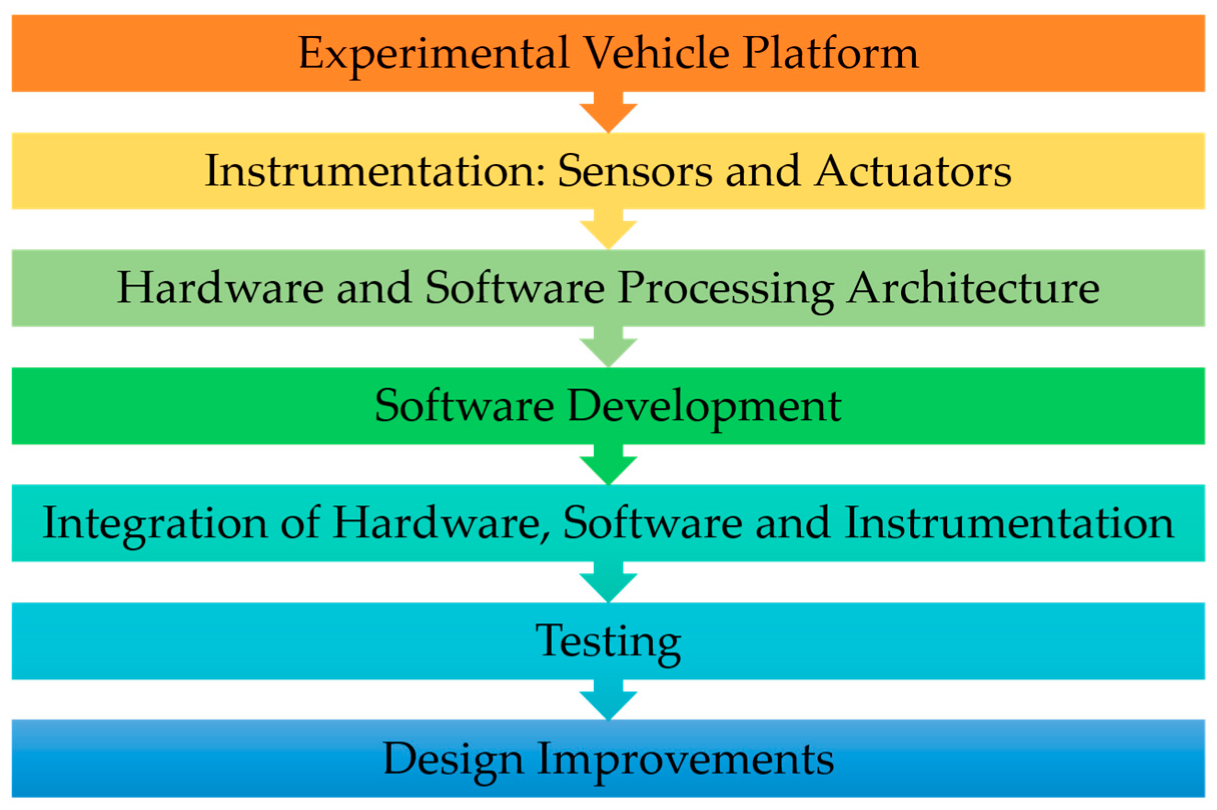
To carry out this work, it was necessary to use a research and development methodology. The development had to fulfill with the proposed work within a margin of 4 weeks. During this time, the research, development, and testing of the vehicle platform had to be carried out with the BC/IL algorithm. This methodology can be seen in
Figure 2.
The methodology describes the stages for the development of this work. The first stages were to define and know the vehicle platform. This platform was already built, so this work was limited to knowing its characteristics and capabilities, which are described in the following section. For the instrumentation, actuators were already defined in the platform, but it was necessary to propose the required sensors to implement the BC/IL algorithm for driving automation.
The next stage was to define the hardware and software for processing. This needed to have the minimum capacity necessary to process DL algorithms and be able to communicate with the sensors and actuators installed on the platform. That is why the Nvidia Jetson AGX Javier met the requirements.
The stages of software development and integration were the next ones. During these stages, it was fundamental the use of ROS and DL frameworks, such as Keras and Tensorflow. The testing stage was made up of several parts, such as data acquisition and neural network training and testing protocol. All of this focused on the proposed route for the vehicle to drive it autonomously.
After obtaining results, it was necessary to analyze and define some design improvements on all stages of the development of this work. These will be reviewed in the analysis, conclusions, and future work sections of this paper.
For all stages of the methodology, it was essential to support it with information found in state-of-the-art developments. All the stages are detailed in the following sections.
5. Experimental Platform
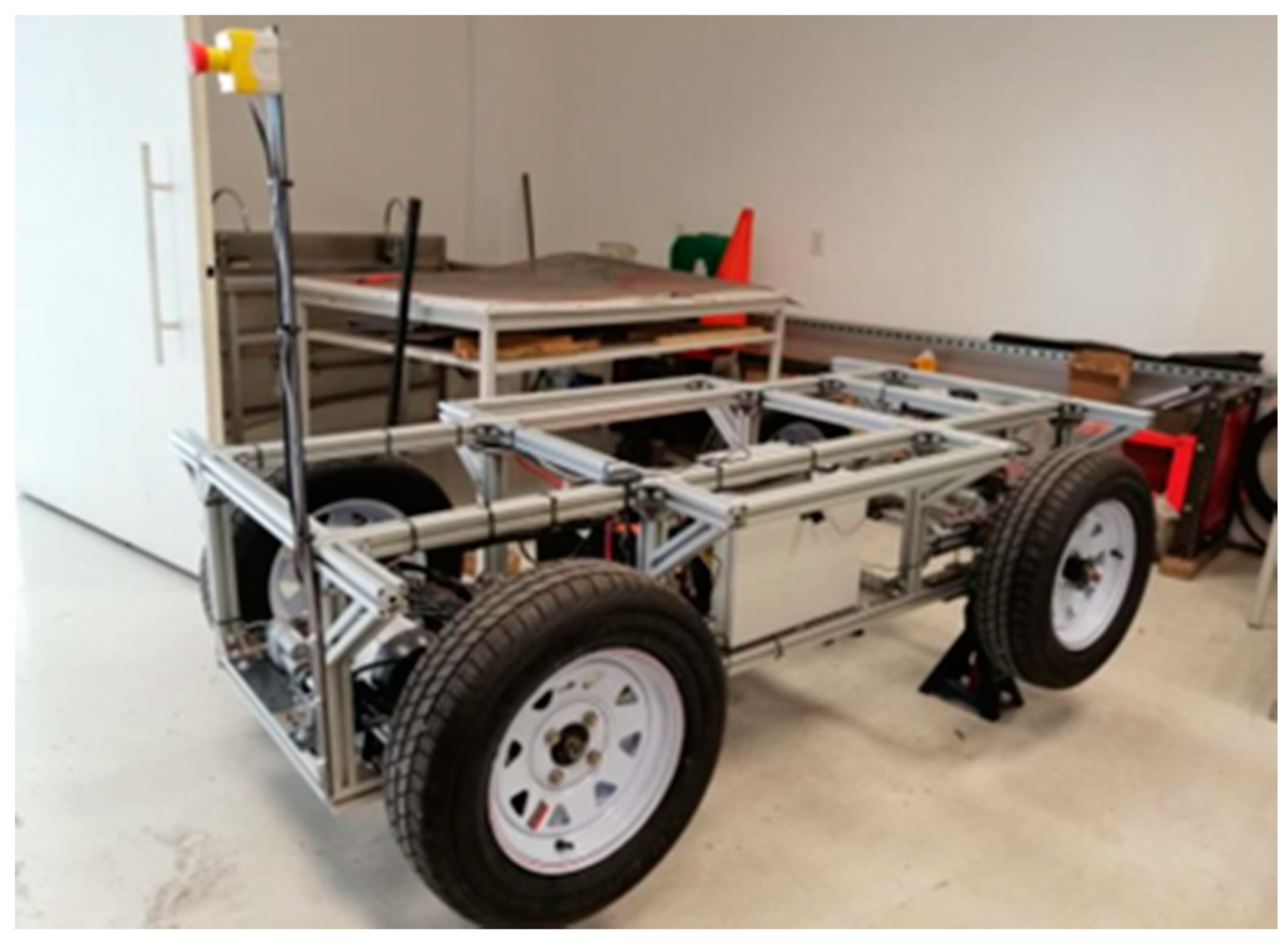
Different add-ons enhance the bare-bones platform so that it can be used for diverse purposes, such as personal transportation or cargo. The electric vehicle’s drive is rear-wheeled. A control box in the rear generates the signals for the open-loop transmission system. This system can set a speed level, rotational direction, and braking. The brakes are triggered with a hysteresis controller system that activates coupled relays.
This system communicates through an RS-232 serial protocol. The vehicle uses an Ackermann distribution with a 30° steering ratio. The steering system uses the same communication protocol as the brakes, while a closed-loop system controls the position. It is also equipped with switches that detect the maximum position on each side. The modular platform can be controlled with an Xbox wireless controller with no electrical or mechanical modifications made to the vehicle. The general technical details of the platform are listed in
Table 3 and an image of the modular platform is depicted in
Figure 3.
This is a minimal system vehicle that can be used for passenger transportation or cargo. It can be further enhanced with sensors and processors to become an AGV.
5.1. Sensors and Instrumentation
The vehicle had three cameras covering the front view. The central processing hardware was a Nvidia Jetson AGX Xavier that oversaw acquiring data, processing it, and turning it into actuator primitives.
The components that were used to accomplish autonomous navigation can be grouped into sensors, processors, and control elements.
Table 4 briefly summarizes these elements.
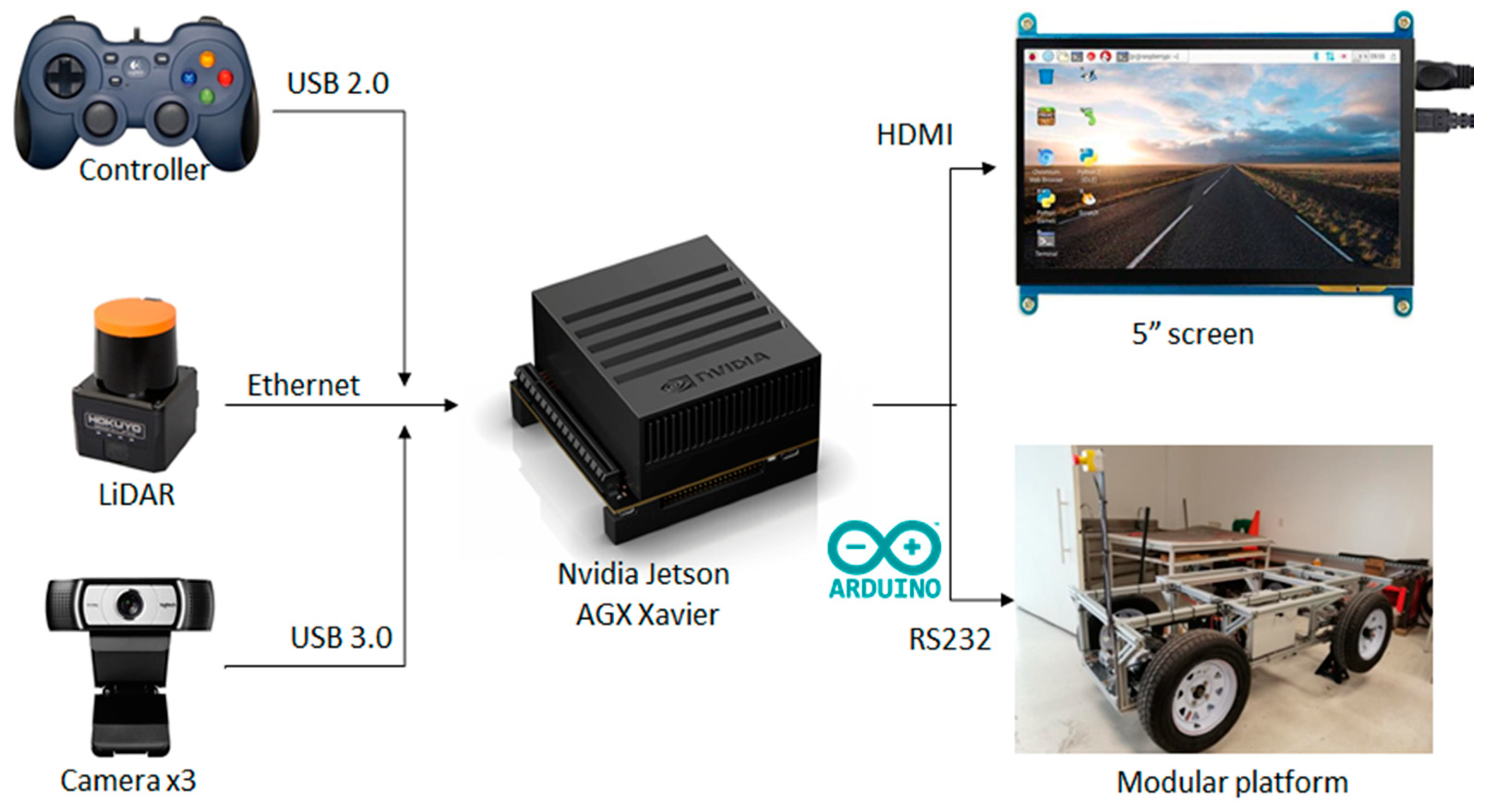
Two types of sensors were used to acquire information from the environment: cameras and a LIDAR. The Logitech cameras used were middle/low range. They provided 720–1080 p images at 30 fps with a 78° field of view (FOV). Their automatic light correction warranties contrasted images, making them a good choice for different outdoor environments. Three of these cameras were used to generate a 150° FOV, as the acquired images from the left and right cameras overlapped the central one. The LIDAR, an active sensor manufactured by Hokuyo, uses a laser source to scan a 270° FOV divided into 1081 steps and a maximum distance of 10 m. It has an angular resolution of 0.25° and a linear accuracy of 40 mm. A full scan takes around 25 ms. The LIDAR was positioned in the center of the vehicle’s front. An F310 Logitech gamepad was used to tele-operate the vehicle’s velocity and Ackerman’s steering angle [
49]. These four sensors along with the gamepad were connected to the AGV’s processor: a Nvidia Jetson AGX Xavier. The cameras were connected through USB-C 3.0 ports, the Hokuyo through an Ethernet connection, and the gamepad via a USB 2.0.
A Nvidia Jetson AGX Xavier and an Atmega 2560 were used as high and low-level controllers, respectively. The Nvidia Jetson AGX Xavier acquired and processed information from the environment and the user. The user’s information was acquired through a mouse, a keyboard, and a gamepad, which were connected to a USB-hub 3.0. The CPU/GPU capabilities of this development kit enable it to perform operations of up to 1100 MHz. Thus, ML algorithms can be easily implemented in this platform. The user can supervise the Nvidia Jetson AGX Xavier through an on-board screen. The developer kit translated its computations into low-level instructions that could be communicated to a microcontroller using an RS232 protocol. An ATmega 2560 microcontroller embedded in an Arduino 2560 shield was used. This microcontroller can handle an intensive use of input-output (IO) peripherals and serial communication protocols. It has enough computational power to implement a basic open-loop and hysteresis control for the speed, braking, and steering systems. The speed system was open loop. Basic digital outputs were enough to activate and deactivate the system. Hysteresis control for the brakes and steering required an Analog-Digital Converter (ADC) and the RS232 communication protocol. The brakes and the steering angle positions were sensed with potentiometers. Typical H-bridges were used to trigger the actuators, which could be halted by a kill switch that interrupted the Vcc. The kill switch was used as an emergency stop.
Figure 4 shows the instrument connection diagram.
5.2. Software Architecture
The Robotics Operating System (ROS) was chosen because of its ease of handling input and output devices, communication protocols, such as RS232 or CAN, and simultaneously running scripts of different programming languages, like Python or C++. ROS is based on nodes that oversee specific tasks, such as communicating with a microcontroller or processing information from a camera. Nodes subscribe or publish information through topics. They can run in parallel, which allows an agile flow of information. Safety nodes were implemented so that whenever a publisher stopped working, the vehicle would make an emergency stop. The ROS facilitated high and low-level algorithm integration. SAE level 1 navigation was achieved with E2E BC/IL. Several expert users drove on the test track to generate the training data. Drivers used the vehicle at different times of the day to get different light conditions. Twelve models were tested in a simulated testbed before being implemented in the vehicle. The AGV was tested on campus in a controlled environment. All the autonomous navigations were successful. The enhancement and automation were carried out in a four-week time span.
The goal of this work was to implement the instrumentation, programming, intelligence, and integration of minimal system requirements to enhance an electric vehicle to an SAE level 1 AGV in less than four weeks. The BC/IL minimum instrumentation proposed in [
15] was used as a basis. A LIDAR sensor was added in order to continuously monitor the distance to the surrounding elements and prevent a collision. This section will go into further detail of the instrumentation, the test track and the DNN architecture.
5.3. Neural Network Architecture
A robust and fast CNN was used to solve the autonomous steering problem of this work. As mentioned in
Section 2, DNNs are the most popular alternatives to train a BC/IL system [
17]. This work’s implementation was inspired by DAVE-2 [
15,
16]. In this model, an image could be loaded to a DNN and yield a steering wheel angle value for the modular platform. Thirteen CNN models were tested before one had the desired driving behavior. The images used as inputs were acquired from the three cameras described in
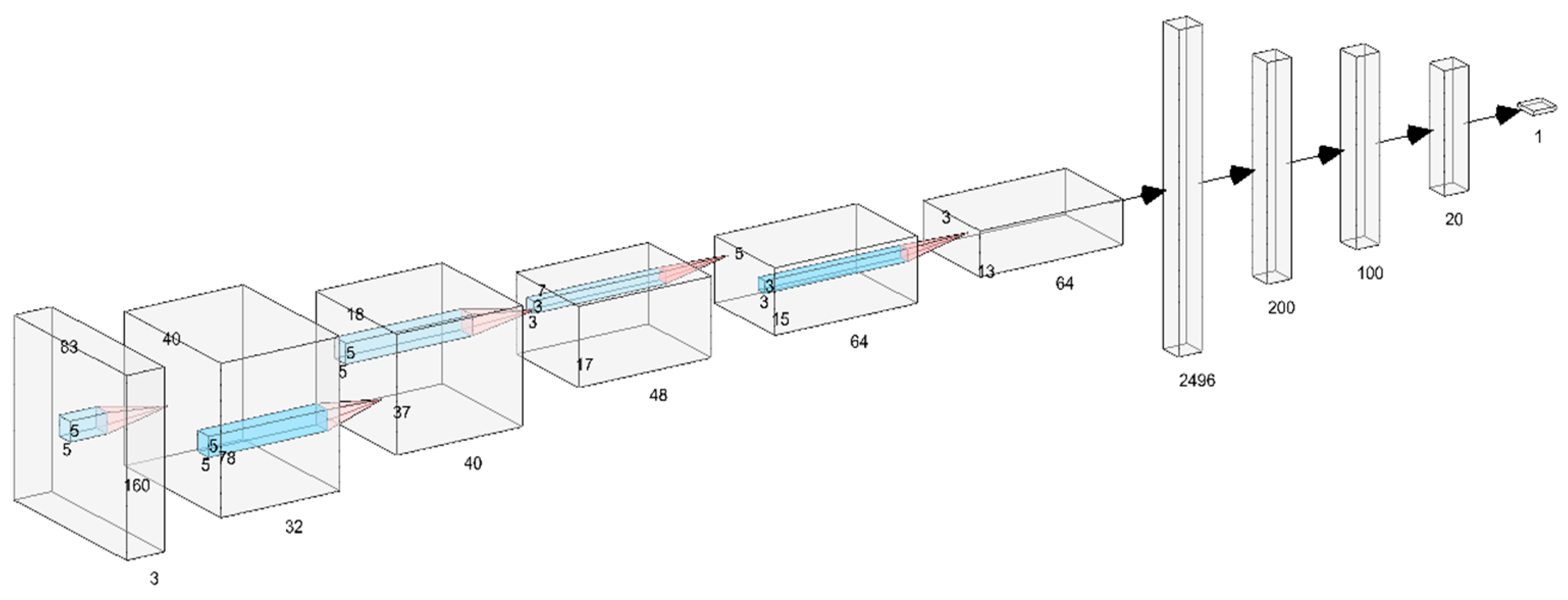
Section 5.1. The images coming from the front central camera were labeled with the steering wheel angle, whereas the ones are coming from the lateral one were labeled with a correction of the steering wheel angle. Each image was an RGB 720 × 480 px. The images were resized and cropped to an 83 × 160 8-bit RGB. As the RGB data had a 0–255 range, it needed to be normalized to a −0.5 to 0.5 range before being fed to the NN. Normalization helped to reduce the processing time and memory usage. The following formula was used to achieve this:
The input layer was followed by five convolutional layers. The first three use 5 × 5-sized filters and the next two 3 × 3. The output was then vectorized to obtain an array of 2496 elements. Then, three fully connected neural layers of 200, 100, and 20 elements were alternated with dropout layers. The dropout layers prevent the system from overfitting [
50]. Convolutional and fully connected layers were activated by Rectified Linear Unit (ReLU) functions, which helped with weight adjustment during the Adam-optimized training stage [
51]. More details of the training process will be described in the following sections. Finally, the one-dimensional layer outputs from −1 to 1 were normalized to the predicted angle.
Figure 5 shows a diagram of the CNN architecture used for this work.
During the training process, different architectures were tested by modifying the convolution filter sizes and the number of neurons, optimizers, and activation functions in order to find the best model, which is the one described above.
5.4. Proposed Route
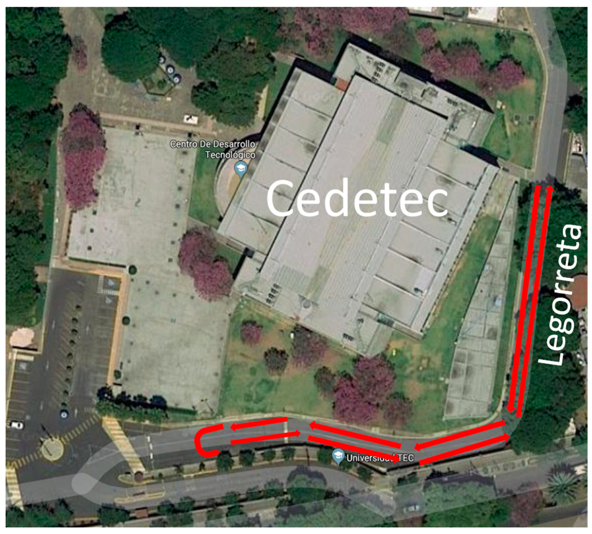
Tecnológico de Monterrey, Campus Ciudad de México is in the south of Mexico City. The campus has internal roads and streets. The traffic and number of pedestrians in these roadways are almost non-existent. Therefore, they represent an excellent option for a controlled and low-risk environment. The chosen 170 m flat road segment is located between the Cedetec and Legorreta buildings. When the roundtrip is considered, the street has two pronounced 90° left/right curves and a 70 m slightly left/right curved way. The roadway is generally in good condition, although it has a few bumps and potholes with poor lane separation. The sidewalk is separated from the road surface by a yellow line. The satellite view of the test track (red) is depicted in
Figure 6. The data acquisition and test phases were held under restricted access to the area and expert supervision.
6. Development
This section will provide details on how the ROS integration, data acquisition, system training, and tests were developed.
6.1. ROS Integration
Hardware architecture described previously in
Section 5.1 was managed by the Robot Operating System (ROS), a collection of open-source software. It provides a wide range of computational tools such as low-level device control, process communication, hardware abstraction, and package management. ROS is based on the computational graph model, which allows a wide range of devices to run the same programs if they comply with some basic hardware specifications. The communication between platforms is straightforward and simple. Each ROS process is called a node, which is jointly interconnected through topics. A node is a hardware or software element that requests or provides data, which can be a single value or clustered elements. Data are sent through topics. An ROS Melodic Morena was used on an Ubuntu 18.04 OS [
52]. Each element described in
Section 5.1 was a node.
The master node was a C++ or Python program used during the data acquisition and testing, respectively. This node subscribed to each input element: cameras (usb_cam), LIDAR (urg_node), and the gamepad (joy). It also published information via RS232 (rosserial) to an ATmega256. The microcontroller was also a node (rosserial_arduino). The master script used OpenCV, cv_bridge, image_transport, and sensor_msgs libraries in order to acquire and process the corresponding information. It receives information from the Nvidia Jetson AGX Xavier, and transforms this information into primitives for the actuators.
For the training and test phases, a template was created. It retrieves and preprocesses information from the input nodes. The camera’s images were switched from an RGB to BGR color palette, then they were resized and cropped. The LIDAR data were continuously compared with a safety factor; if the current measurement was within ±10% of the safety factor, the vehicle would try to avoid the threat. However, if the measurement was not acceptable, the platform would stop and enter lock mode. The published data were sent using the RS232 communication protocol. The speed interval went from zero up to 30 km/h. It was normalized in a −4 to 9 interval. This range was chosen according to the documentation of the modular platform. The sign of the integer determined the motion direction: negative backward and positive forward. According to the documentation, the steering values of the platform range from −20° to 20°. The microcontroller produces a Pulse-Width Modulation (PWM) signal, with a duty cycle that is proportional to the steering angle. The minimum value maps to the leftmost steering value (−20°) with the value of 400, while the maximum is the rightmost, (20°) with a value of 800. The brakes were activated with a Boolean. The data were gathered into a single string that contained the speed, steering, and braking setpoints. The microcontroller receives the string and parses it to acquire the desired setpoints. As the data were already in primitive values, the ATmega256 uses them as references for the open-loop or hysteresis control.
For the training phase, synchronized data from each node were properly indexed and stored. This data was later used to train the CNN. The ROS low latency minimizes the time difference between samples coming from different devices. However, the process cannot be considered real-time. During the testing phase, data was added to the CNN and the output was published to the actuator. The trained model uses libraries for Python and C++ contained in Tensorflow and Keras [
53]. The user supervises the proper performance of the system. A safety node was implemented using the gamepad, such that a button can be pressed to stop the software from executing and lock the modular platform.
Figure 7 shows the overall ROS integrated system.
The initial tests were performed with a high range computer with a Nvidia GPU. The ROS node integration worked smoothly. However, during the migration to the Nvidia Jetson AGX Xavier, several compatibility issues emerged. The first one to appear was CUDA, a parallel computing platform and programming model from NVIDIA, which is optimized to work with a GPU or a CPU. Nevertheless, our development kit is a mixture of both. A lite version needed to be installed to solve the problem. Another issue was the interaction between Python versions. ROS uses Python 2.7, while all the AI software uses Python 3.7. Separate virtual environments were needed to make all the libraries work together.
6.2. Data Acquisition and Preprocessing
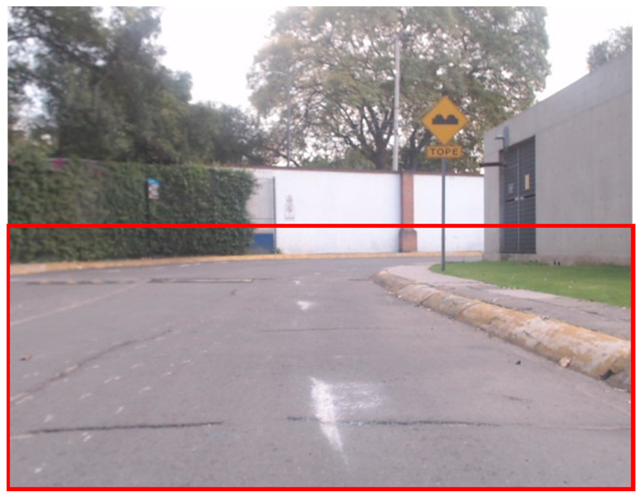
The hardware architecture and the ROS-based system were tested in the lab before testing them with the vehicle. The LIDAR response worked as expected. No further modifications were needed. The image acquisition system required several iterations for it to work correctly. During the initial tests, some images were missing or broken. The initial supposition was that ROS was unable to handle data acquisition from three cameras simultaneously. However, when testing the template with different cameras, this hypothesis was dismissed. Individual response time tests with RGB 720 × 480 images were performed. The results showed that the number of frames per second (fps) of each camera was different: 18, 20, and 60, respectively. The simplest solution was to sample all the cameras at the slowest rate (18 fps). This way, the same number of simultaneous images could be acquired and saved along with the current steering angle. The images were preprocessed to select an area of interest and this area was taken into consideration when training the CNN. Such an area can be seen in
Figure 8.
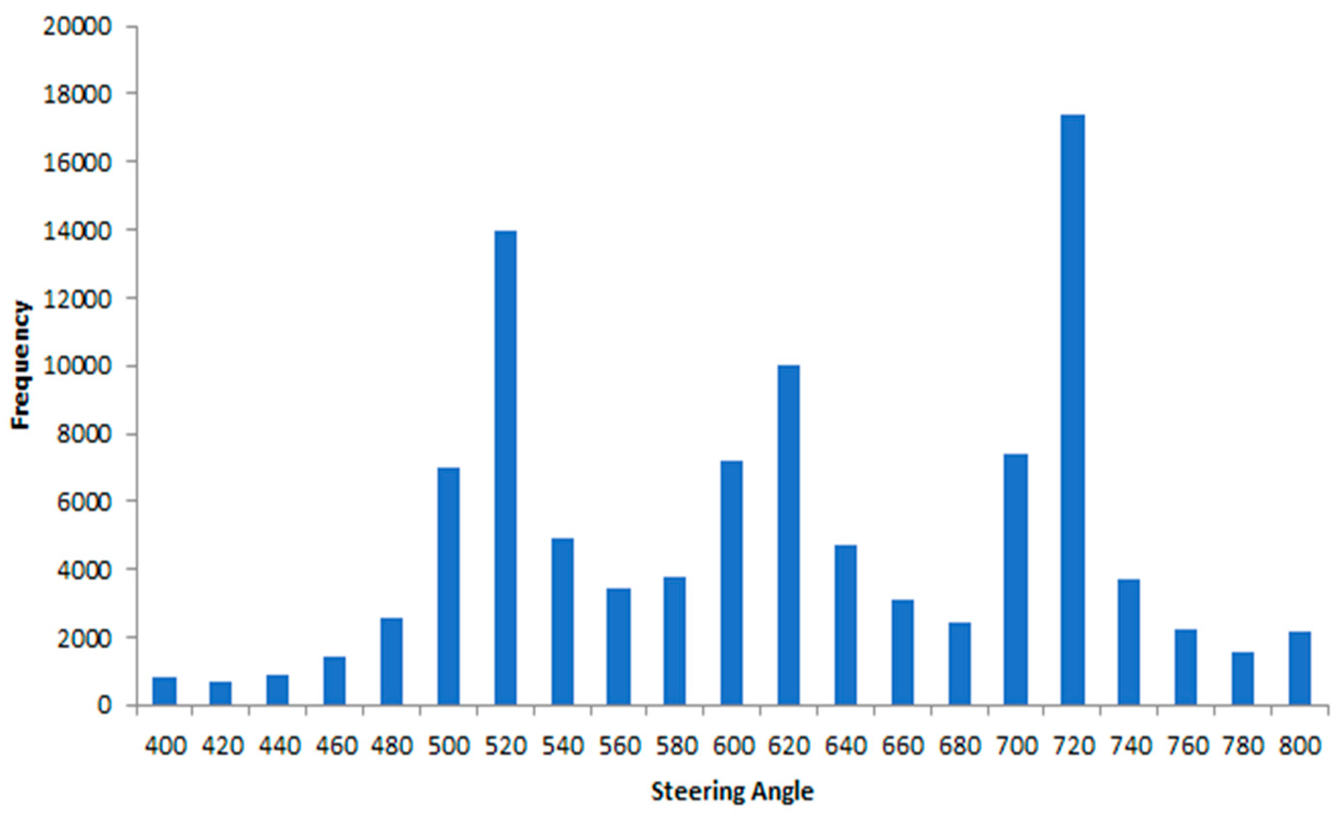
In order to successfully train a CNN, enough training data is required. The data should be as diverse and complete as possible in order for the CNN to throw a useful result. For this purpose, the test track was recorded on seven round trips. More than 100 thousand images were collected. Each image was bound with its respective steering angle. The navigation of the vehicle was made in right-hand traffic. For the purpose of assuring suitable training data for the CNN, steering angles collected as raw data were normalized and augmented. A histogram of raw data for such steering angles is shown in
Figure 9. It can be seen that there is a slight bias in the histogram, which might lead to an unsuccessful training.
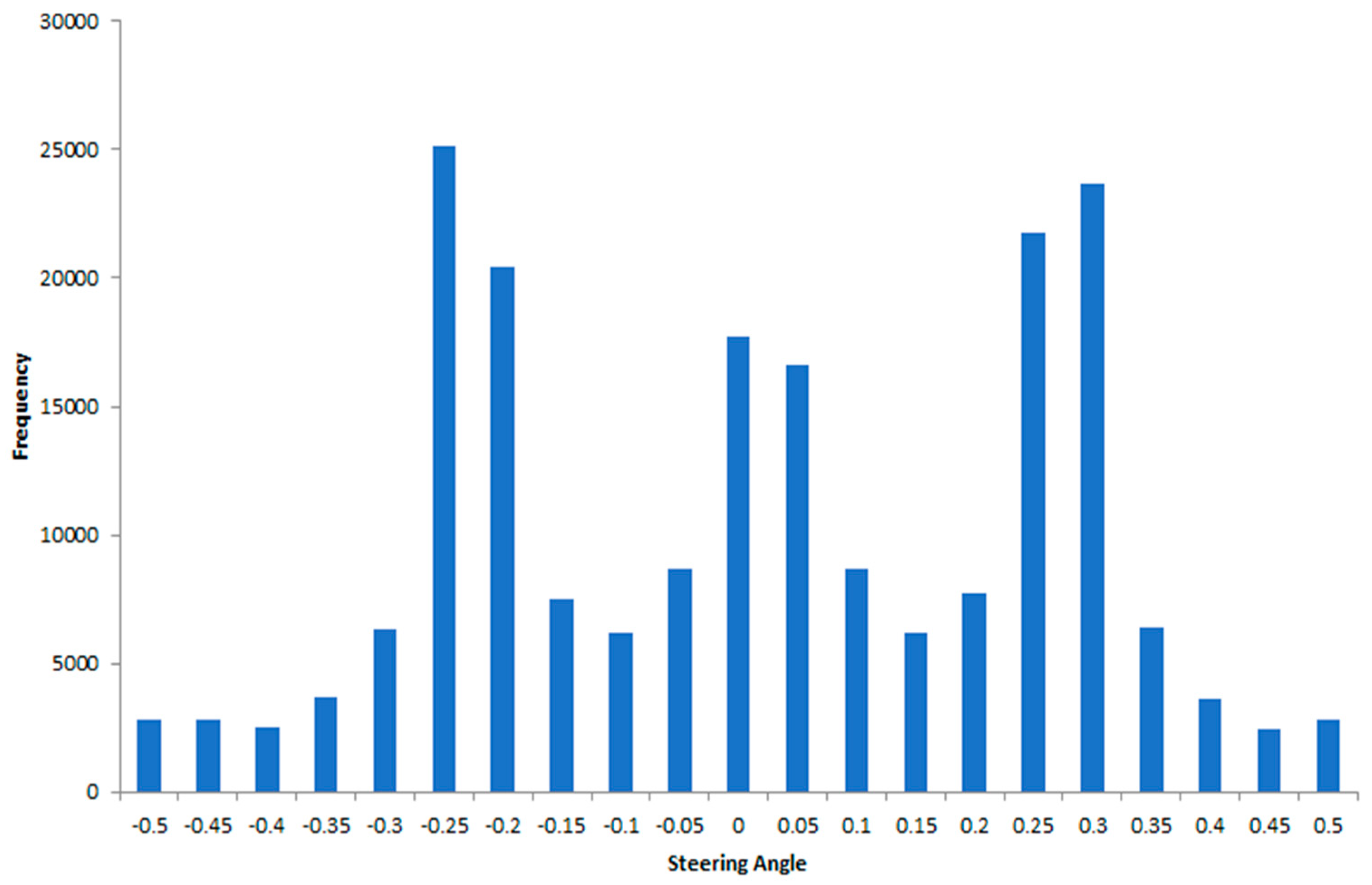
In order to minimize the effect of this bias, prior to training we introduced data augmentation. That is, we horizontally flipped all images and multiplied the normalized steering data times −1. As a result, we had a dataset twice as big as the original one (206,726 images with its corresponding steering angle). This way, the CNN could generalize more efficiently against any bias that is taken towards any given steering angle. The histogram of the data after augmentation and normalization can be seen in
Figure 10.
The histogram demonstrates how the augmentation and normalization of the data help give greater symmetry to the amount of data per label. This allows to reduce the probability of bias of the system towards a certain type of response and lets the model generalize data in a better way during training.
A total of 103,363 synchronized data points were used for the training stage. This dataset was split in Keras into training (70%) and validation (30%) subsets. The percentages used are used in state-of-the-art works. The separation of data can be seen in more detail in
Table 5.
6.3. Training Process
The training data contains individual images sampled from the video along with the corresponding steering command. Training with human driver data is not enough. In order to successfully navigate the road and avoid leaving the lane, the network must also learn how to recover from mistakes.
In order to facilitate this improved model, images of the car from different perspectives are added to the training data, including images from the center of the lane and images taken from different angles of the road.
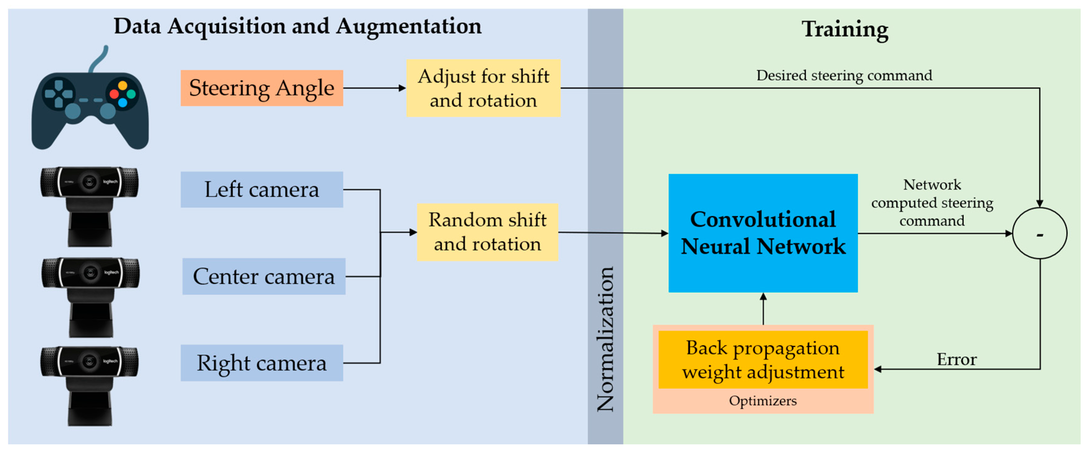
A block diagram of the training system developed is shown in
Figure 11. The images are inputted into a CNN that calculates a proposed steering angle, which is compared to the desired angle for that image. The resulting error is used to update the weights of the CNN and to bring the CNN output closer to the desired output. The weight adjustment is performed using a backpropagation algorithm and optimizers such as the Adams, Keras, and Tensorflow libraries. It is important to note that all the data prior to training enter a normalization layer of the CNN, with the aim of making training more efficient and reducing the computer’s memory usage.
The training process required a careful selection of parameters, which included the optimizer, batch size, number of time values, and separation of data between validation and training. Adam, Stochastic Gradient Descent (SGD), and Adadelta optimizers were used in the different models.
The loss is calculated by training and validation. Unlike accuracy, loss is not a percentage. It is a summation of the errors made for each example in training or validation sets. The loss value is usually lower in the training set. The important thing to take care of is that there is no overfitting by observing a general increase in the loss value instead of a decrease. The number of epochs varied depending on the loss drop difference, but all the models were run between 12 and 25 times before the loss value stopped decreasing. Loss values are usually closer to 0. The lower the loss, the better the model (unless the model is overfitted to the training data). The data separation was always the same, with 70% training and 30% validation.
Training times vary depending on the amount of data and their resolution, the CNN architecture, the computing power, the framework efficiency, and other parameters. The basic architecture of the navigation NN was based on the one proposed by Bojarski [
15]. The training was carried out on a computer with the following specifications: 6th generation of Intel i7 processor, RAM: 32 GB, GPU: Nvidia 1080 GTX, with 8 GB dedicated memory. The training was conducted in the GPU and the training times were between 14 and 32 min. The Deep Learning framework used was Keras 2.3 integrated with TensorFlow 1.14 running in Python.
6.4. Algorithm Evaluation and Testing
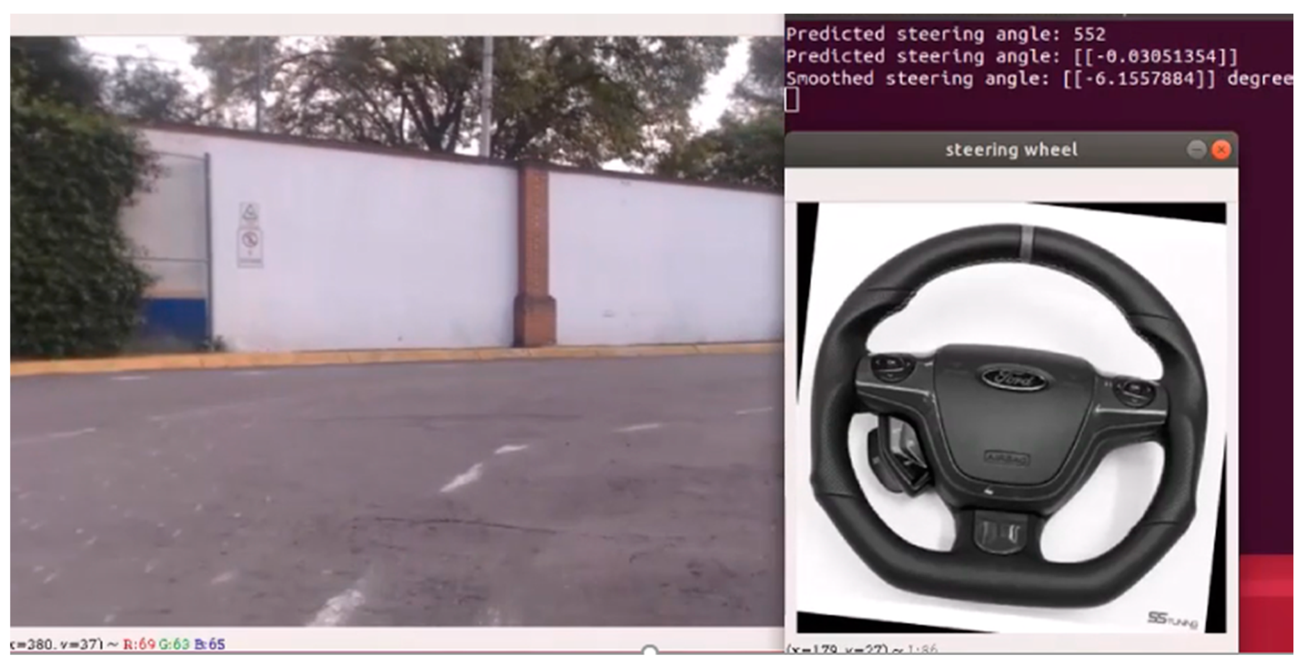
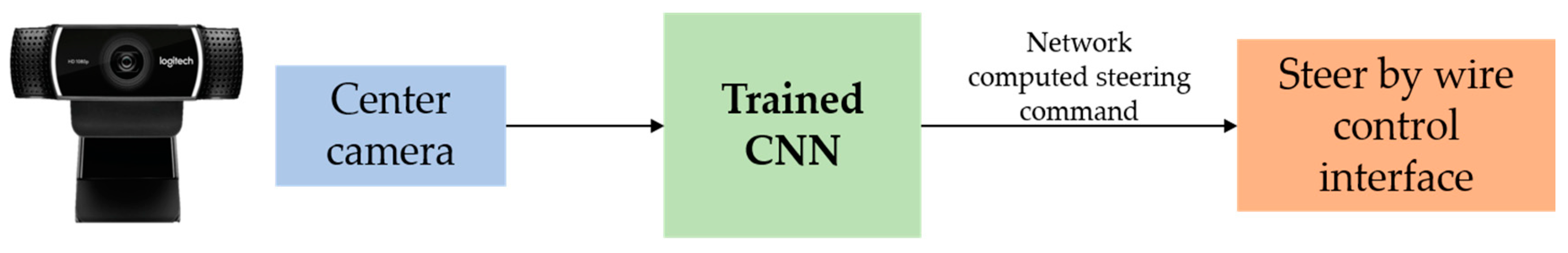
The following protocol and criteria were used to validate the model performance.
The information flow starts with image acquisition of the front camera. The next stages were performed in the Nvidia Jetson AGX Xavier preprocessing and model operation. The model will predict a steering angle, which will later be sent to the microcontroller.
Figure 13 shows this process.
7. Results and Discussion
Throughout the training and data acquisition process, 13 different CNN models were trained. Each one was evaluated by the test protocol contained in
Section 6.4.
Table 6 shows the evaluation of every model. The accuracy is obtained with the final value that Keras prints during the training. This value is calculated through the Mean Absolute Error (
MAE) [
54], which is expressed by the equation:
The final value is the percentage of MAE that the model has with all the training data (training + validation sets). The following stages of the protocol result in more qualitative results through the observation of the model’s performance with the test video and the real trials on the test route.
In the four weeks of work, three data acquisitions were performed to increase the amount of training data in search of an improvement in the prediction of the model. In the first capture, 15,276 images were acquired with their corresponding steering angles, the second reached 43,157 data points, and the last capture generated 103,363 data points. As can be seen, the efficiency of data capture between the three data acquisitions and with software and hardware corrections in the acquisition systems was improved. This improved the system performance and accuracy in predicting the angle.
Another important question in the development of the models was whether or not to use data augmentation, since it was considered that it could generate noise during training. However, after evaluation it was determined that the augmentation quantitatively and qualitatively improved the performance of the model.
As mentioned in the previous section, there were three test stages, each described in
Section 6.4, with the results shown in
Table 6. Since the first four models did not meet the requirements of stage 1, the following stages were not performed. Tests in stage 2 of models 5 to 13 obtained the results shown in
Figure 12. At this test stage, it was evaluated if the models made sudden accurate predictions of movement, with particular attention to the part of the main curve of the in-campus circuit. This evaluation had a qualitative nature during driving. In stage 3, it was decided to physically test the model considering the safety aspects mentioned in
Section 6.4. Only the best three models passed this test. The objective was to finish the in-campus circuit with the least human intervention. As mentioned before, the speed was controlled all the time by the driver for safety purposes.
7.1. Best Model Results
CNN model 13 was the one that obtained the best results in the tests, especially in stage 3 of the test, where an automated steering direction of the entire in-campus circuit was achieved with almost no human intervention to modify the steering angle of the vehicle. The architecture of this model is the one presented in
Section 5.3. This model was trained with the Adam optimizer for 14 epochs. The duration of training was 28 min and 37 s with a high capacity computer, whose characteristics are mentioned in
Section 6.3. This model was trained with 206,726 images obtained by the augmentation of the 103,363 original data points with their respective steering wheel angles.
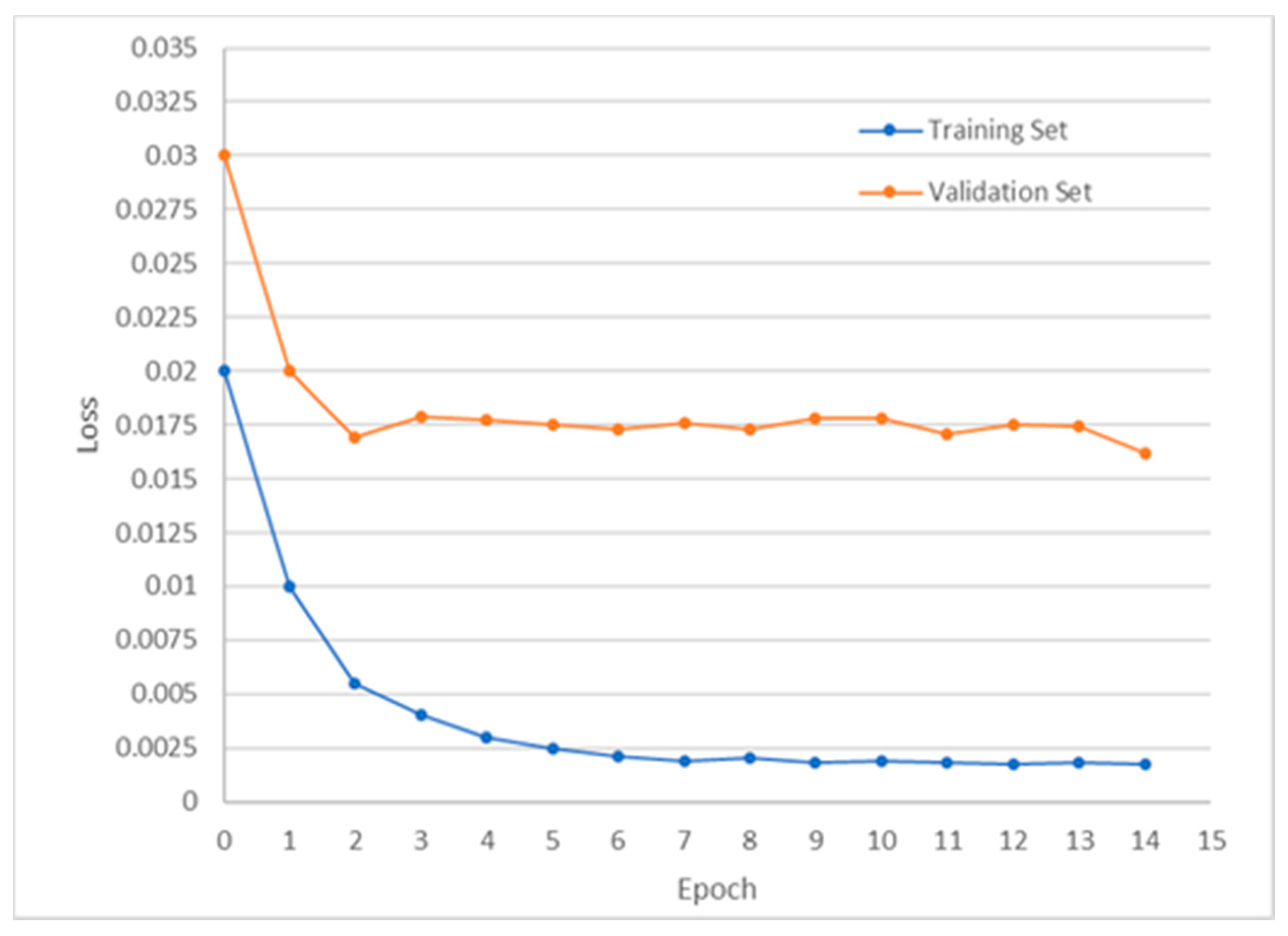
An important parameter to consider during training is loss, as shown in
Figure 14 for all training epochs.
The training set efficiency was verified by the ever-decreasing values of loss across the epochs. As for the validation set, a mild improvement was noticed but it had a mostly constant performance all over the training. Although there was a low improvement in the loss for the validation set, the values for the validation set are lower than 0.02 units. As mentioned above, a loss value close to 0 and with a decreasing trend indicates a well-trained model. The loss value of the validation set is higher than the training set is normal. The important thing is to protect the model from overfitting by keeping its value as low as possible with a decreasing trend.
The platform thus can be expected to develop as planned when the model starts running as a node in the ROS topics, instead of being directed by the remote controller. From the loss plot, it is important to note that the loss value generally declines, since an increasing trend would suggest overfitting the model.
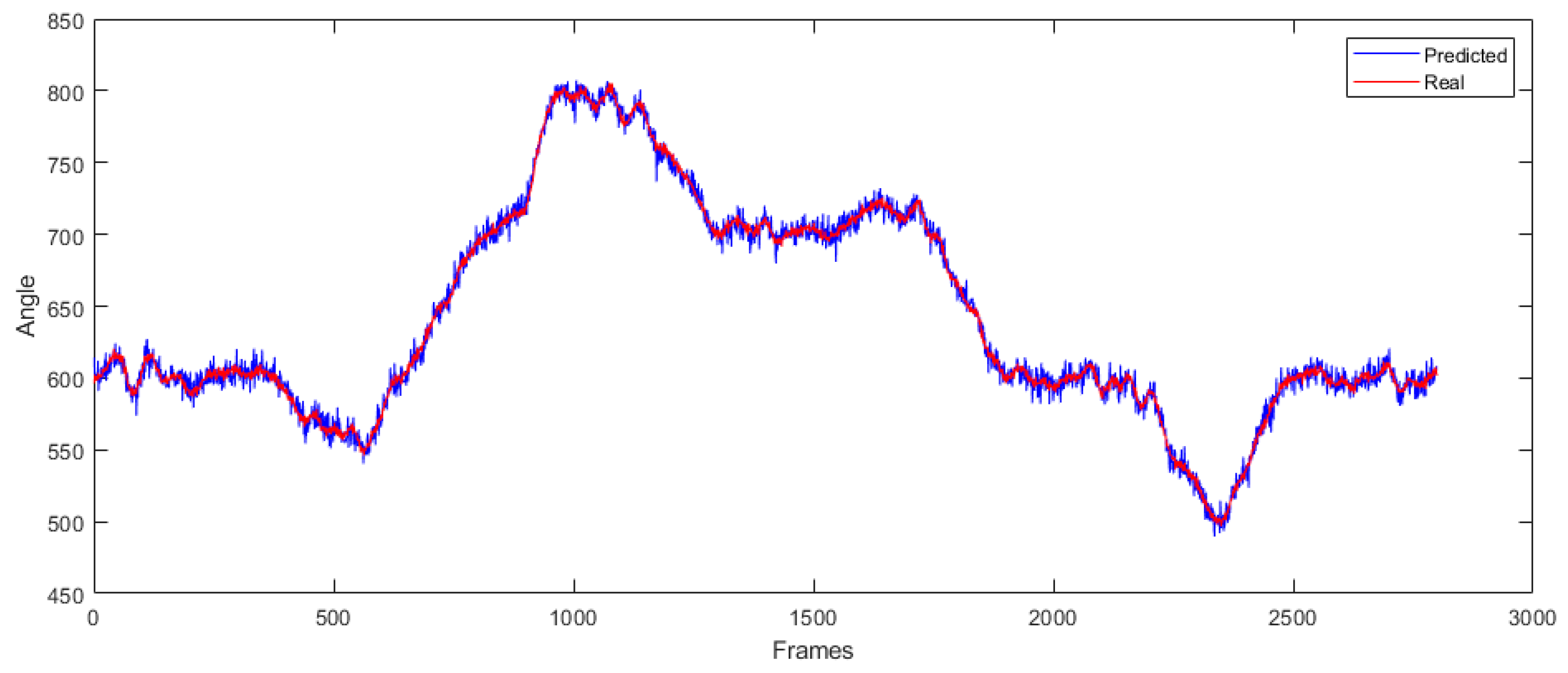
Figure 15 shows the prediction of the steering wheel angle made by our CNN model against the ground truth obtained from the training data. This prediction was generated with one of the datasets in which it was trained in order to observe the precision obtained by the model.
A certain “noise” can be observed in the prediction, which is reduced by applying a moving average filter when the predicted value is sent to the steering wheel actuator. This filter is expressed by the equation:
where
y is the new output,
x is the predicted output, and
M is the number of data points used. This model, as it is trained on a fixed route, presents excellent precision with the data in the tests. However, if a more generalized prediction for the model is desired, it is necessary to increase the variety and amount of training data. This model obtained a 94.5% accuracy with the training data. Although other models had a higher percent accuracy, this model performed better in the other stages of the evaluation protocol.
7.2. Shadow Effects
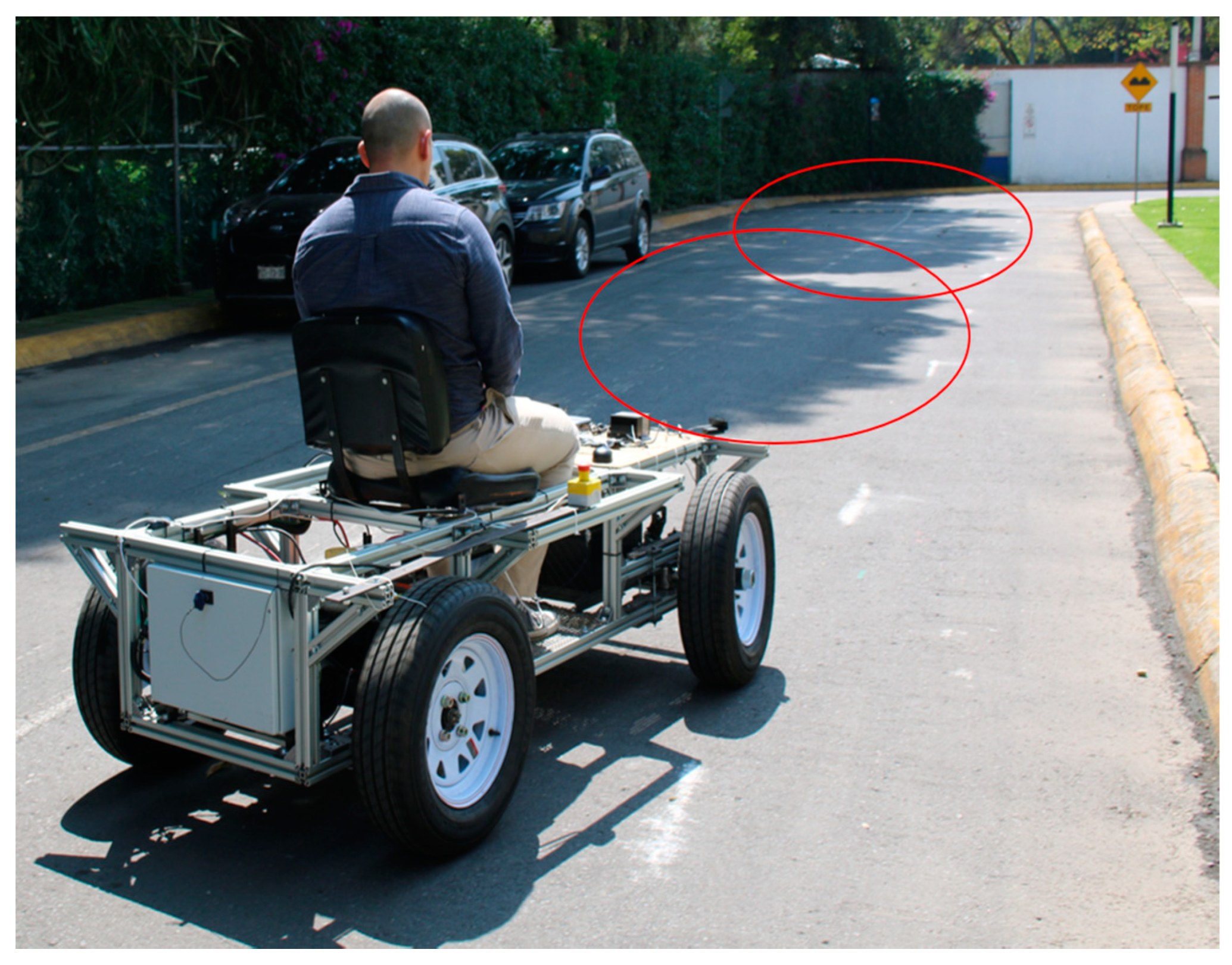
The training set was demonstrated to be well developed. In the field, the platform behaved perfectly under similar conditions to the ones used for training. During the week of training and data acquisition, the weather was cloudy. However, it was sunny during the presentation. This condition negatively impacted the performance, because the shadows increased the amount of noise in the system. An example of these shadows can be seen in
Figure 16.
During the presentation, the angle of the sun diminished the effect of the shadows. In order to fix the effect of the shadows, data must be additionally collected during various times and under varying weather conditions, which was not possible during the week of data collection. The platform completed the entire proposed route seen in
Figure 6 and completed three circuits with the only human interaction being that needed to accelerate the vehicle.
8. Conclusions
Technological advancements in computing power allow for the development of more efficient, more practical, and lower cost autonomous vehicles. Several of the algorithms used today, especially in the area of Artificial Intelligence, were developed more than 50 years ago, but technological advancements allow for their implementation in this particular application. Research and development are crucial to the improvement of robust systems that can mimic human behavior.
The development and improvement of electric and intelligent vehicles either for private or public use in industry or transportation services is a disruptive issue nowadays. All development must be carried out around an intelligent electromobility ecosystem. For this, the development of various vehicle platforms for different purposes must be conducted as part of this ecosystem. This is how the concept of the Automated Guided Modular Vehicle was created.
Driving a vehicle is a very complex task. Therefore, the desire that a machine completes such a chore is not simple. Although autonomous driving began to have efficient implementations in the previous decade, it still has areas of improvement that this work seeks to satisfy.
The algorithm of BC/IL allowed generating a practical and efficient solution in the time limit. The results were as expected: the modular AGV was able to navigate the proposed route. Even so, it is necessary to continue developing more complex models, with the option of being able to use reinforced learning or unsupervised learning. This can help generate a more complex and more efficient solution. Even so, it is important to keep the safety criteria in mind, especially if the tests are carried out in a real environment with a platform that has the ability to cause physical damage.
Likewise, the use of a platform not designed in-house brought us advantages and disadvantages. There were several parts of the design that could be considered as a plug and play, which was beneficial in the process. The development of autonomous vehicles is something that technological development and the current computing is allowing to become more efficient, practical, and of lower cost. The origins of several of the algorithms used today, especially in the area of Artificial Intelligence, were developed more than 50 years ago but can be implemented in a real way thanks to the current technology. Nonetheless, development and research are needed to improve them in order to mimic human behavior more precisely.
This work contains the successful implementation of a minimum system for a SAE Level 1 modular autonomous vehicle. This type of vehicle begins to be a differential in the industry and in the implementation of personal transport systems. That is why this work also contributes to the generation and development of the concept of a low-cost modular AGV, capable of driving autonomously on certain fixed routes, and been part of the current trends of mobility services and smart cities. The system is based on ROS and has hardware and software elements. Data acquisition from hardware elements with different sampling rates was achieved. Minimal data curation was performed due to the highly efficient data collection system. High- and low-level algorithms were implemented, such that they were efficient in time and computational resources. Our work contributes as a practical implementation in the controlled environment of behavioral cloning and imitation learning algorithms. The vehicle successfully navigated on a 300 m track. It evaded vehicles and potholes and drove in right-hand traffic.
The most significant relevance of this work is to show that an autonomous navigation system can be implemented in diverse hardware and vehicular platforms, as long as they have a standardized software platform. This opens the opportunity to generate a test environment for other research use and contribute as an open HW-SW solution to the scientific community in the area.
Work Contributions
After the development of this work, different contribution points were defined. After analyzing state-of-the-art technology, it can be observed that there are not many implementations of automated vehicles in the transportation of people or cargo. The design of the vehicle, although it was not part of this work, meets the general concept of an AGV with autonomous driving capacity level 1 and in future work, level 2. This type of vehicle begins to have a significance in the industry with an implementation in personal transport systems. This work contributes to the generation of a low-cost modular AGV capable of driving autonomously on certain fixed routes.
Likewise, our work contributes as an example of a practical implementation of the BC/IL algorithm in a real environment. This algorithm has excellent capabilities and facilities that allowed the completion of the work in the 4-week limit. Even so, the algorithm needs to become more robust or be complemented in a way for it to reach higher levels of autonomy, even if these complements generate a higher cost solution.
9. Future Work
The development of this work had several limitations due to the time of 4 weeks of development. Future work that improves the design and functionality of the AVG is described in the following part:
Improve the autonomous driving algorithm that allows leading with disturbances (shadows and lights in the image), that modify the performance of the algorithm.
Optimize code and hardware architecture to allow faster processing. Incorporating other algorithms and models options with higher performance, for example, using Deep Convolutional Inverse Graphics Network (DCIGN) architectures [
55].
The automation proposed in this work is limited to level 1 of the SAE scale. A future job will be able to go up to a level 2, which allows automating the acceleration and braking of the vehicular model.
An improvement in the longitudinal dynamics of the vehicle, acceleration, and braking stages are safety aspects that must be taken into account for the improvement of the future design.
The vertical dynamics of the vehicle will have to be revised to improve overall the mechanical response of the autonomous system. In case of emergency evasion, the system must respond as fast as possible.
The on-board electronics will need to be upgraded for viable operation; a Printed Circuit Board (PCB), in order to dispose of all the wires inside the vehicle’s control box, is proposed, since this gives additional noise to the sensor measurements. The Arduino is no longer going to be used. Instead, the STM32L496ZGT6P board with the Nucleo-144 microcontroller will help have a more efficient signal control and processing. This also because of its ROS compatibility software and its ARM architecture capable of managing an 80 MHz frequency [
56].
These are the highlights for improvement in the future work of the Automated Guided Modular Vehicle proposed and developed in this paper.
Author Contributions
Conceptualization, L.A.C.-R., R.B.-M., H.G.G.-H., J.A.R.-A. and E.C.G.-M.; methodology, L.A.C.-R., R.B.-M. and E.C.G.-M.; software, L.A.C.-R., R.B.-M., J.A.R.-A. and E.C.G.-M.; validation, L.A.C.-R., R.B.-M. and E.C.G.-M.; investigation, L.A.C.-R., R.B.-M., H.G.G.-H., J.A.R.-A. and E.C.G.-M.; resources, R.A.R.-M., H.G.G.-H., J.A.R.-A. and M.R.B.-B.; data curation, L.A.C.-R.; writing—original draft preparation, L.A.C.-R., R.B.-M., R.A.R.-M., E.C.G.-M. and M.R.B.-B.; writing—review and editing, L.A.C.-R., R.B.-M., H.G.G.-H., J.A.R.-A., R.A.R.-M., E.C.G.-M. and M.R.B.-B.; supervision, R.A.R.-M., H.G.G.-H., J.A.R.-A. and M.R.B.-B.; project administration, M.R.B.-B.; funding acquisition, R.A.R.-M., J.A.R.-A. and M.R.B.-B. All authors have read and agreed to the published version of the manuscript.
Funding
Funding was provided by Tecnologico de Monterrey (Grant No. a01333649 and a00996397) and Consejo Nacional de Ciencia y Tecnologia (CONACYT) by the scholarship 850538 and 679120.
Acknowledgments
We appreciate the support and collaboration of Miguel de Jesús Ramírez Cadena, Juan de Dios Calderón Nájera, Alejandro Rojo Valerio, Alfredo Santana Díaz and Javier Izquierdo Reyes; without their help, this project would not have been carried out.
Conflicts of Interest
The authors declare no conflict of interest.
Appendix A
Table A1.
List of acronyms.
Table A1.
List of acronyms.
| Acronym | Definition | Acronym | Definition |
|---|
AD
AGV | Autonomous Driving
Automated Guided Vehicles | ADAS
AI | Advanced Driving Assistance System
Artificial Intelligence |
| ARM | Advanced RISC Machines | AV | Autonomous Vehicle |
| BC | Behavioral Cloning | CAN | Controller Area Network |
| CNN | Convolutional Neural Network | CPU | Central Processing Unit |
| DL | Deep Learning | DNN | Deep Neural Network |
| DRL | Deep Reinforcement Learning | E2E | End to End |
| FCN | Fully Convolutional Network | FOV | Field of View |
| GPU | Graphic Processing Unit | IL | Imitation Learning |
| LIDAR | Laser Imaging Detection and Ranging | LSTM | Long-Short Term Memory |
| ML | Machine Learning | NN | Neural Network |
| RAM | Random Access Memory | RNN | Recurrent Neural Network |
| ROS | Robot Operating System | SAE | Society of Automotive Engineers |
| SGD | Stochastic Gradient Descent | TaaS | transport as a Service |
| USB | Universal Serial Bus | | |
References
- Curiel-Ramirez, L.A.; Izquierdo-Reyes, J.; Bustamante-Bello, R.; Ramirez-Mendoza, R.A.; de la Tejera, J.A. Analysis and approach of semi-autonomous driving architectures. In Proceedings of the 2018 IEEE International Conference on Mechatronics, Electronics and Automotive Engineering (ICMEAE), Cuernavaca, Mexico, 26–29 November 2018; pp. 139–143. [Google Scholar]
- Mercy, T.; Parys, R.V.; Pipeleers, G. Spline-based motion planning for autonomous guided vehicles in a dynamic environment. IEEE Trans. Control Syst. Technol. 2018, 26, 6. [Google Scholar] [CrossRef]
- Fazlollahtabar, H.; Saidi-Mehrabad, M. Methods and models for optimal path planning. Autonomous Guided Vehicles; Springer: Cham, Switzerland, 2015. [Google Scholar] [CrossRef]
- Urmson, C.; Anhalt, J.; Bagnell, D.; Baker, C.; Bittner, R.; Dolan, J.; Duggins, D.; Ferguson, D.; Galatali, T.; Geyer, C.; et al. Tartan Racing: A Multi-Modal Approach to the DARPA Urban Challenge; DARPA: Pittsburgh, PA, USA, 2007.
- Veres, S.; Molnar, L.; Lincoln, N.; Morice, P. Autonomous vehicle control systems—A review of decision making. Proc. Inst. Mech. Eng. I J. Syst. Control Eng. 2011, 225, 155–195. [Google Scholar] [CrossRef]
- SAE International J3016. Available online: https://www.sae.org/standards/content/j3016_201401/ (accessed on 12 April 2020).
- SAE International. SAE J3016: Taxonomy and Definitions for Terms Related to Driving Automation Systems for On-Road Motor Vehicles; SAE International: Troy, MI, USA, 15 June 2018; Available online: https://saemobilus.sae.org/content/j3016_201806 (accessed on 6 January 2020).
- Shuttleworth, J. SAE Standards News: J3016 Automated-Driving Graphic Update. 7 January 2019. Available online: https://www.sae.org/news/2019/01/sae-updates-j3016-automated-driving-graphic (accessed on 6 January 2020).
- Kocić, J.; Jovičić, N.; Drndarević, V. Sensors and sensor fusion in autonomous vehicles. In Proceedings of the 2018 26th Telecommunications Forum (TELFOR), Belgrade, Serbia, 20–21 November 2018; pp. 420–425. [Google Scholar]
- Goodfellow, I.; Bengio, Y.; Courville, A. Deep Learning; The MIT Press: Cambridge, MA, USA, 2017; Available online: https://www.deeplearningbook.org (accessed on 5 December 2019).
- Aggarwal, C.C. Neural Networks and Deep Learning; Springer International Publishing: Cham, Switzerland, 2018; ISBN 978-3-319-94462-3. [Google Scholar]
- Chowdhuri, S.; Pankaj, T.; Zipser, K. MultiNet: Multi-modal multi-task learning for autonomous driving. In Proceedings of the 2019 IEEE Winter Conference on Applications of Computer Vision, Hilton Waikoloa Village, HI, USA, 7–11 January 2019. [Google Scholar]
- Teichmann, M.; Weber, M.; Zöllner, M.; Cipolla, R.; Urtasun, R. MultiNet: Real-time joint semantic reasoning for autonomous driving. In Proceedings of the 2018 IEEE Intelligent Vehicles Symposium (IV), Changshu, Suzhou, China, 26–30 June 2018. [Google Scholar]
- Al-Qizwini, M.; Barjasteh, I.; Al-Qassab, H.; Radha, H. Deep learning algorithm for autonomous driving using GoogLeNet. In Proceedings of the IEEE Intelligent Vehicles Symposium (IV), Redondo Beach, CA, USA, 11–14 June 2017. [Google Scholar]
- Sengupta, S.; Basak, S.; Saikia, P.; Paul, S.; Tsalavoutis, V.; Atiah, F.; Ravi, V.; Peters, A. A review of deep learning with special emphasis on architectures, applications and recent trends. arXiv 2019, arXiv:1905.13294. [Google Scholar] [CrossRef]
- Shrestha, A.; Mahmood, A. Review of deep learning algorithms and architectures. IEEE Access 2019, 7, 53040–53065. [Google Scholar] [CrossRef]
- Bojarski, M.; Del Testa, D.; Dworakowski, D.; Firner, B.; Flepp, B.; Goyal, P.; Jackel, L.D.; Monfort, M.; Muller, U.; Zhang, J.; et al. End to end learning for self-driving cars. arXiv 2016, arXiv:1604.07316. [Google Scholar]
- Bojarski, M.; Yeres, P.; Choromanska, A.; Choromanski, K.; Firner, B.; Jackel, L.; Muller, U. Explaining how a deep neural network trained with end-to-end learning steers a car. arXiv 2017, arXiv:1704.07911. [Google Scholar]
- Teti, M.; Barenholtz, E.; Martin, S.; Hahn, W. A systematic comparison of deep learning architectures in an autonomous vehicle. arXiv 2018, arXiv:1803.09386. [Google Scholar]
- Schikuta, E. Neural Networks and Database Systems; University of Vienna, Department of Knowledge and Business Engineering: Wien, Austria. arXiv 2008, arXiv:0802.3582. [Google Scholar]
- Roza, F. End-to-End Learning, the (Almost) Every Purpose ML Method. Towards Data Science, Medium. 31 May 2019. Available online: https://towardsdatascience.com/e2e-the-every-purpose-ml-method-5d4f20dafee4 (accessed on 15 January 2020).
- Torabi, F.; Warnell, G.; Stone, P. Behavioral Cloning from Observation; The University of Texas at Austin, U.S. Army Research Laboratory: Austin, TX, USA. arXiv 2018, arXiv:1805.01954. [Google Scholar]
- Sallab, A.E.; Abdou, M.; Perot, E.; Yogamani, S. Deep reinforcement learning Framework for autonomous driving. In Proceedings of the IS&T International Symposium on Electronic Imaging 2017, Hyatt Regency San Francisco Airport Burlingame, Burlingame, CA, USA, 29 January–2 February 2017. [Google Scholar] [CrossRef]
- Fridman, L.; Jenik, B.; Terwilliger, J. Deeptraffic: Crowdsourced hyperparameter tuning of deep reinforcement learning systems for multi-agent dense traffic navigation. arXiv 2019, arXiv:1801.02805. [Google Scholar]
- Sallab, A.E.; Abdou, M.; Perot, E.; Yogamani, S. End-to-end deep reinforcement learning for lane keeping assist. arXiv 2016, arXiv:1612.04340. [Google Scholar]
- Shalev-Shwartz, S.; Shammah, S.; Shashua, A. Safe, multi-agent, reinforcement learning for autonomous driving. arXiv 2016, arXiv:1610.03295. [Google Scholar]
- Ramezani Dooraki, A.; Lee, D.-J. An end-to-end deep reinforcement learning-based intelligent agent capable of autonomous exploration in unknown environments. Sensors 2018, 18, 3575. [Google Scholar] [CrossRef]
- Wu, K.; Abolfazli Esfahani, M.; Yuan, S.; Wang, H. Learn to steer through deep reinforcement learning. Sensors 2018, 18, 3650. [Google Scholar] [CrossRef] [PubMed]
- Zhang, J.; Cho, K. Query-efficiente imitation learning for end-to-end autonomous driving. arXiv 2016, arXiv:1605.06450. [Google Scholar]
- Pan, Y.; Cheng, C.; Saigol, K.; Lee, K.; Yan, X.; Theodorou, E.A.; Boots, B. Agile autonomous driving using end-to-end deep imitation learning. arXiv 2019, arXiv:1709.07174. [Google Scholar]
- Tian, Y.; Pei, K.; Jana, S.; Ray, B. DeepTest: Automated testing of deep-neural-network-driven autonomous cars. In Proceedings of the IEEE/ACM 40th International Conference on Software Engineering (ICSE), Gothenburg, Sweden, 27 May–3 June 2018. [Google Scholar]
- Xu, H.; Gao, Y.; Yu, F.; Darrell, T. End-to-end learning of driving models from large-scale video datasets. In Proceedings of the IEEE Conference on Computer Vision and Pattern Recognition, Honolulu, HI, USA, 21–26 July 2017. [Google Scholar]
- Cortes Gallardo-Medina, E.; Moreno-Garcia, C.F.; Zhu, A.; Chípuli-Silva, D.; González-González, J.A.; Morales-Ortiz, D.; Fernández, S.; Urriza, B.; Valverde-López, J.; Marín, A.; et al. A comparison of feature extractors for panorama stitching in an autonomous car architecture. In Proceedings of the 2019 IEEE International Conference on Mechatronics, Electronics and Automotive Engineering (ICMEAE), Cuernavaca, Mexico, 26–29 November 2019. [Google Scholar]
- Riedmiller, M.; Montemerlo, M.; Dahlkamp, H. Learning to drive a real car in 20 minutes. In Proceedings of the 2007 Frontiers in the Convergence of Bioscience and Information Technologies, Jeju City, Korea, 11–13 October 2007; pp. 645–650. [Google Scholar]
- Pomerleau, D.A. ALVINN: An Autonomous Land Vehicle in a Neural Network; Technical Report CMU-CS-89-107; Carnegie Mellon University: Pittsburgh, PA, USA, 1989. [Google Scholar]
- Lecun, Y.; Cosatto, E.; Ben, J.; Muller, U.; Flepp, B. DAVE: Autonomous Off-Road Vehicle Control Using End-to-End Learning; DARPA-IPTO: Arlington, VA, USA, 2004.
- Kocić, J.; Jovičić, N.; Drndarević, V. Driver behavioral cloning using deep learning. In Proceedings of the 17th International Symposium INFOTEH-JAHORINA (INFOTEH), East Sarajevo, Republika Srpska, 21–23 March 2018; pp. 1–5. [Google Scholar]
- Haavaldsen, H.; Aasbo, M.; Lindseth, F. Autonomous vehicle control: End-to-end learning in simulated urban environments. arXiv 2019, arXiv:1905.06712. [Google Scholar]
- Kocić, J.; Jovičić, N.; Drndarević, V. An end-to-end deep neural network for autonomous driving designed for embedded automotive platforms. Sensors 2019, 19, 2064. [Google Scholar] [CrossRef]
- Bechtel, M.G.; McEllhiney, E.; Kim, M.; Yun, H. DeepPicar: A low-cost deep neural network-based autonomous car. arXiv 2018, arXiv:1712.08644. [Google Scholar]
- Curiel-Ramirez, L.A.; Ramirez-Mendoza, R.A.; Carrera, G.; Izquierdo-Reyes, J.; Bustamante-Bello, M.R. Towards of a modular framework for semi-autonomous driving assistance systems. Int. J. Interact. Des. Manuf. 2019, 13, 111. [Google Scholar] [CrossRef]
- Mehta, A.; Adithya, S.; Anbumani, S. Learning end-to-end autonomous driving using guided auxiliary supervision. arXiv 2018, arXiv:1808.10393. [Google Scholar]
- Navarro, A.; Joerdening, J.; Khalil, R.; Brown, A.; Asher, Z. Development of an autonomous vehicle control strategy using a single camera and deep neural networks. In SAE Technical Paper; SAE: Warrendale, PA, USA, 2018; No. 2018-01-0035. [Google Scholar]
- Pan, X.; You, Y.; Wang, Z.; Lu, C. Virtual to real reinforcement learning for autonomous driving. arXiv 2017, arXiv:1704.03952. [Google Scholar]
- Chen, C.; Seff, A.; Kornhauser, A.; Xiao, J. DeepDriving: Learning affordance for direct perception in autonomous driving. In Proceedings of the IEEE International Conference on Computer Vision, Santiago, Chile, 7–13 December 2015. [Google Scholar]
- Curiel-Ramirez, L.A.; Ramirez-Mendoza, R.A.; Izquierdo-Reyes, J.; Bustamante-Bello, R.; Tuch, S.A.N. Hardware in the loop framework proposal for a semi-autonomous car architecture in a closed route environment. Int. J. Interact. Des. Manuf. 2019, 13, 111. [Google Scholar] [CrossRef]
- Huval, B.; Wang, T.; Tandon, S.; Kiske, J.; Song, W.; Pazhayampallil, J.; Andriluka, M.; Rajpurkar, P.; Migimatsu, T.; Cheng-Yue, R.; et al. An empirical evaluation of deep learning on highway driving. arXiv 2015, arXiv:1504.01716. [Google Scholar]
- Viswanath, P.; Nagori, S.; Mody, M.; Mathew, M.; Swami, P. End to end learning based self-driving using JacintoNet. In Proceedings of the 2018 IEEE 8th International Conference on Consumer Electronics (ICCE), Berlin, Germany, 2–5 September 2018. [Google Scholar]
- Jing-Shan, Z.; Xiang, L.; Zhi-Jing, F.; Dai, J. Design of an ackermann-type steering mechanism. Inst. Mech. Eng. J. Mech. Eng. Sci. 2013, 227, 2549–2562. [Google Scholar]
- Srivastava, N.; Hinton, G.; Krizhevsky, A.; Sutskever, I.; Salakhutdinov, R. Dropout: A simple way to prevent neural networks from overfitting. J. Mach. Learn. Res. 2014, 15, 1929–1958. [Google Scholar]
- Kingma, D.P.; Adam, J.B. A method for stochastic optimization. Cornell University, Computer Science, Machine Learning. In Proceedings of the 3rd International Conference of Learning Representations, San Diego, CA, USA, 7–9 May 2015. [Google Scholar]
- ROS.org. Robotic Operating System Melodic Morenia. Available online: http://wiki.ros.org/melodic (accessed on 25 November 2019).
- TensorFlow Core, Keras Documentation. Python. March 2015. Available online: https://keras.io/ (accessed on 5 October 2019).
- Sammut, C.; Webb, G.I. Mean absolute error. In Encyclopedia of Machine Learning; Springer: Boston, MA, USA, 2011. [Google Scholar]
- Kulkarni, T.D.; Whitney, W.; Kohli, P.; Tenenbaum, J.B. Deep Convolutional Inverse Graphics Network; Cornell University: Ithaca, NY, USA, March 2019. [Google Scholar]
- STMicroelectronics. NUCLEO-L496ZG. Available online: https://www.st.com/en/evaluation-tools/nucleo-l496zg.html (accessed on 10 January 2020).
Figure 1.
Deep Reinforcement Learning (DRL) diagram.
Figure 1.
Deep Reinforcement Learning (DRL) diagram.
Figure 2.
Research and development methodology.
Figure 2.
Research and development methodology.
Figure 3.
Modular platform built by Campus Puebla.
Figure 3.
Modular platform built by Campus Puebla.
Figure 4.
Instrument connection diagram.
Figure 4.
Instrument connection diagram.
Figure 5.
Final CNN architecture.
Figure 5.
Final CNN architecture.
Figure 6.
Test track satellite view.
Figure 6.
Test track satellite view.
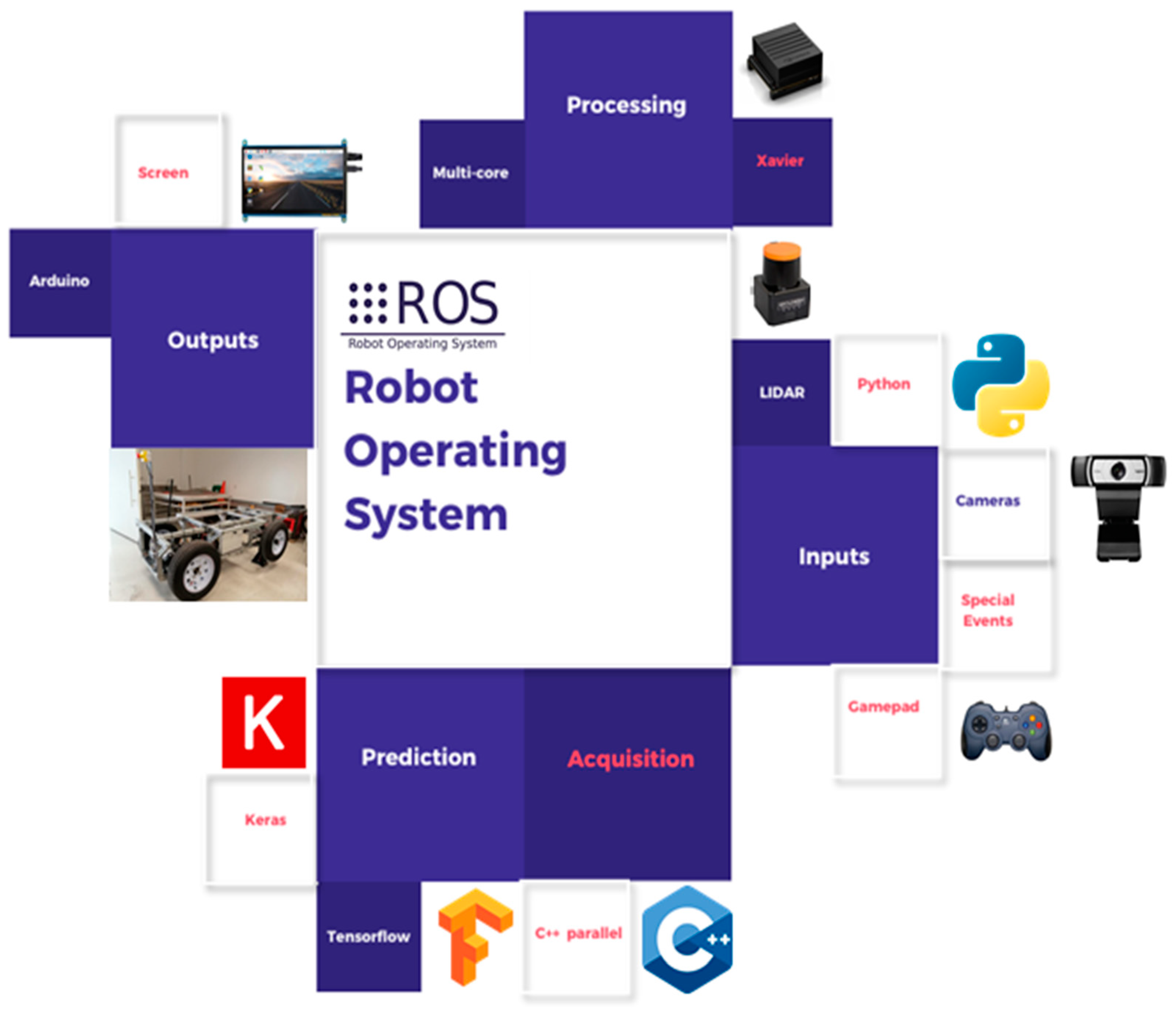
Figure 7.
Robot Operating System (ROS) integration diagram.
Figure 7.
Robot Operating System (ROS) integration diagram.
Figure 8.
Image acquired and area of interest.
Figure 8.
Image acquired and area of interest.
Figure 9.
Histogram of the raw data acquisition.
Figure 9.
Histogram of the raw data acquisition.
Figure 10.
Histogram of the data after the normalization and augmentation process.
Figure 10.
Histogram of the data after the normalization and augmentation process.
Figure 11.
Diagram for the data acquisition and training of the neural network.
Figure 11.
Diagram for the data acquisition and training of the neural network.
Figure 12.
Stage 2 of a test, prediction of the model with unseen video.
Figure 12.
Stage 2 of a test, prediction of the model with unseen video.
Figure 13.
Diagram for the prediction of the steering wheel angle of the vehicle.
Figure 13.
Diagram for the prediction of the steering wheel angle of the vehicle.
Figure 14.
Loss plot of model 13 during training.
Figure 14.
Loss plot of model 13 during training.
Figure 15.
Prediction of the steering angle in a sample dataset.
Figure 15.
Prediction of the steering angle in a sample dataset.
Figure 16.
Examples of shadows on the day of the final presentation.
Figure 16.
Examples of shadows on the day of the final presentation.
Table 1.
Levels of driving automation based on the Society of Automotive Engineers (SAE) J3016 [
6,
7,
8].
Table 1.
Levels of driving automation based on the Society of Automotive Engineers (SAE) J3016 [
6,
7,
8].
| SAE Levels | Driver Tasks | Vehicle Tasks | Examples |
|---|
| 0 | The driver has the main control even though some of the automated systems are engaged.
The driver must supervise the environment and the system to interfere as he requires it. | The systems work only as momentary assistance providing warnings. | Blindspot warnings, lane departure warnings, parking alerts assistance. |
| 1 | The vehicle has partial control and assistance in the steering OR brake/acceleration. | Lane centering OR adaptive cruise control. |
| 2 | The vehicle controls the steering and brake/acceleration in specific circumstances. | Lane centering AND adaptive cruise control at the same time. |
| 3 | Passive passengers when automated driving is engaged. The driver needs to intervene upon the system request. | The vehicle has autonomous driving in limited conditions and will not operate unless all the conditions are met. | Traffic jam and highway chauffeur. |
| 4 | Passive passengers when automated driving is engaged. The passenger never takes over control. | Local driverless taxi (pedals or steering wheel is optional). |
| 5 | The vehicle has driving control under all conditions. | Robo taxi or full autonomous car (pedals and steering wheel are not required). |
Table 2.
Summary of state-of-the-art Deep Learning (DL) approaches.
Table 2.
Summary of state-of-the-art Deep Learning (DL) approaches.
| Authors | DNN Architecture | Summary | Type of Application |
|---|
| Kocíc, J.; Jovičíc, N.; Drndarevíc, V. | CNN | Implementation of driver behavioral cloning using deep learning in a unity simulator based on a Nvidia CNN network [37]. | Simulation approach |
| Haavaldsen, H.; Aasbo, M.; Lindseth, F. | CNN, CNN-LSTM | Proposal of two architectures for an end-to-end system for driving: a traditional CNN and a CNN extended design combining with a LSTM. All running in the Carla simulator [38]. | Simulation approach |
| Kocíc, J.; Jovičíc, N.; Drndarevíc, V. | CNN | An end-to-end Deep Neural Network for autonomous driving designed for Embedded Automotive Platforms on the Udacity’s Simulator [39]. | Simulation approach |
| Pan, Y.; Cheng, C.; Saigol, K.; Lee, K.; Yan, X.; Theodorou, E.A.; Boots, B. | CNN | Implementation of an agile autonomous driving using End-to-End Deep Imitation Learning on an embedded small kart platform [28]. | Embedded small-scale Automotive platform |
| Bechtel, M.G.; McEllhiney, E.; Kim, M.; Yun, H. | CNN | The development of DeepPicar is a Low-cost DNN based autonomous car platform built on a Raspberry Pi 3 [40]. | Embedded small-scale Automotive platform |
| Kocíc, J.; Jovičíc, N.; Drndarevíc, V. | CNN, ResNet | Overview of sensors and Sensor Fusion in Autonomous Vehicles with a development on embedded platforms [7]. | Subsystem design and proposal |
| Curiel-Ramirez, L.A.; Ramirez-Mendoza, R.A.; Carrera, G. et al. | CNN | Proposal and design of a modular framework for semi-autonomous driving assistance systems for a real scale automotive platform [41]. | Subsystem design and approach |
| Mehta, A.; Adithya, S.; Anbumani, S. | CNN, ResNet | A Multi-task Learning framework on a simulation and cyber-physic platform is proposed for driving assistance [42]. | Real-world and simulated fused environments |
| Navarro, A.; Joerdening, J.; Khalil, R.; Brown, A.; Asher, Z. | CNN, RNN | Development of an Autonomous Vehicle Control Strategy Using a Single Camera and Deep Neural Networks. Different architectures, including Recurrent Neural Networks (RNN), are used in a simulator and then on a real autonomous vehicle [43]. | Real-world and simulated fused environments |
| Pan, X.; You, Y.; Wang, Z.; Lu, C. | CNN, FCN | Computer vision system that generates real view images from virtual environment pictures taken from a simulator. This is applied for data augmentation for autonomous driving systems using Fully Convolutional Networks (FCN) [44]. | Real-world and simulated fused environments |
| Chen, C.; Seff, A.; Kornhauser, A.; Xiao, J. | CNN | DeepDriving is a learning affordance for direct perception in autonomous driving. The base training was made in simulation and tested with real environment pictures for lane change direction [45]. | Real-world and simulated fused environments |
| Curiel-Ramirez, L.A.; Ramirez-Mendoza, R.A.; Izquierdo-Reyes, J. et al. | CNN, any | The proposal and implementation of a framework with hardware-in-the-loop architecture to improve autonomous car computer vision systems via simulation and hardware integration [46]. | Real-world and simulated fused environments |
| Zhang, J.; Cho, K. | CNN | Improvement of the imitation learning for end-to-end autonomous driving using a Query-Efficiente learning method [27]. | Algorithm learning optimization |
| Xu, H.; Gao, Y.; Yu, F.; Darrell, T. | FCN, LSTM | An FCN-LSTM model proposal for end-to-end learning on driving models using large-scale video datasets [30]. | Algorithm learning optimization |
| Tian, Y.; Pei, K.; Jana, S.; Ray, B. | CNN, RNN | DeepTest is a systematic testing tool for automatically detecting erroneous behaviors of DNN-driven vehicles that can potentially lead to fatal crashes [29]. | Algorithm learning optimization |
| Huval, B.; Wang, T.; Tandon, S.; et al. | CNN | An empirical evaluation of DNN models detecting lane lines in highway driving [47]. | DL models testing in real environments |
| Viswanath, P.; Nagori, S.; Mody, M.; Mathew, M.; Swami, P. | CNN | An end-to-end driving performance test in a highway environment. Additionally, a proposal of an DNN architecture named JacintoNet compared to VGG architecture [48]. | DL models testing in real environments |
| Al-Qizwini, M.; Barjasteh, I.; Al-Qassab, H.; Radha, H. | CNN | Presents a DL algorithm development for autonomous driving using GoogLeNet for highway environments. The system predicts the position of front vehicles [12]. | DL models testing in simulated environments |
Table 3.
Modular vehicle platform technical characteristics.
Table 3.
Modular vehicle platform technical characteristics.
| Transmission |
|---|
| Vcc | 48 V |
| Power | 1000 W |
| Max Speed | 40 km/h |
| Workload | 800 kg |
| Brakes |
| Activation time | 1.5 s |
| Steering |
| Full steering time | 10 s |
| Turning radius | 4.08 m |
| Steering angle | 30° |
Table 4.
Sensors, processors, and control elements.
Table 4.
Sensors, processors, and control elements.
| Sensors |
|---|
| Camera | Logitech | C920 HD pro webcam, 1080 p |
| LIDAR | Hokuyo UST-10LX | 10 m range, 1081 steps, 270° coverage |
| Processors |
| CPU/GPU | Nvidia Jetson AGX Xavier | 512-core Volta GPU, 8-core ARM, 32 GB RAM |
| Microcontroller | ATmega2560 | 54 IO pins, 15 PWM channels, 16 ADC, 256 KB flash memory |
| Controllers |
| H-bridge | L298 | Dual full-bridge driver, 4A, 12 V |
Table 5.
Dataset distribution for training.
Table 5.
Dataset distribution for training.
| | Training | Validation | Total |
|---|
| Number of Samples | 72,354 | 31,009 | 103,363 |
| Percentage | 70% | 30% | 100% |
Table 6.
Summary of the results of the training.
Table 6.
Summary of the results of the training.
| CNN Model | Data Quantity | Data Augmentation | Stage 1 [Train Accuracy] | Test Stage 2 [Test Data] | Test Stage 3 [Real Test] |
|---|
| 1 | 15,276 | no | 85.4% | no | no |
| 2 | 30,552 | yes | 89.2% | no | no |
| 3 | 15,276 | no | 87.7% | no | no |
| 4 | 30,552 | yes | 91.6% | poor | no |
| 5 | 43,157 | no | 92.3% | regular | no |
| 6 | 86,314 | yes | 94.5% | regular | no |
| 7 | 43,157 | no | 92.3% | regular | no |
| 8 | 86,314 | yes | 94.5% | regular/good | no |
| 9 | 103,363 | no | 93.3% | good | no |
| 10 | 206,726 | yes | 94.6% | good | regular |
| 11 | 103,363 | no | 93.8% | very good | good |
| 12 | 206,726 | yes | 94.5% | best | best |
| 13 | 206,726 | yes | 94.3% | good | no |
© 2020 by the authors. Licensee MDPI, Basel, Switzerland. This article is an open access article distributed under the terms and conditions of the Creative Commons Attribution (CC BY) license (http://creativecommons.org/licenses/by/4.0/).

 ,
, 


