Hyperspectral Superpixel-Wise Glioblastoma Tumor Detection in Histological Samples

Abstract

The combination of hyperspectral imaging (HSI) and digital pathology may yield more accurate diagnosis. In this work, we propose the use of superpixels in HS images for combining regions of pixels that can be classified according to their spectral information to classify glioblastoma (GB) brain tumors in histologic slides. The superpixels are generated by a modified simple linear iterative clustering (SLIC) method to accommodate HS images. This work employs a dataset of H&E (Hematoxylin and Eosin) stained histology slides from 13 patients with GB and over 426,000 superpixels. A linear support vector machine (SVM) classifier was performed on independent training, validation, and testing datasets. The results of this investigation show that the proposed method can detect GB brain tumors from non-tumor samples with average sensitivity and specificity of 87% and 81%, respectively. The overall accuracy of this method is 83%. The study demonstrates that hyperspectral digital pathology can be useful for detecting GB brain tumors by exploiting spectral information alone on a superpixel level.

1. Introduction

Digital and computational pathology utilizes digitized images, typically RGB, of histology specimens for the creation of algorithms to aid pathologists in the diagnosis of diseases [1]. There may be information in the electromagnetic spectrum, both visible and beyond, that could be beneficial. Therefore, hyperspectral (HS) digital histology has emerged to explore if it can provide better diagnostic information than RGB (Red, Green, and Blue) imagery. Hyperspectral imaging (HSI) obtains the spectral data of an object using a HS optical sensor and is label-free [2], which can be applied readily to digitized histology.

The main advantage of HSI is the possibility of exploiting both the spatial and the spectral information of the HS data. Although HSI has shown good performance in the detection of different diseases in histopathological applications, this technology still has to face different challenges. One of those challenges is related to the heterogeneity in image processing methods used to extract information from the HS data. Most of these image processing methods consist of application of Machine Learning (ML) methods. There are two main types of ML approaches. In feature learning approaches, the methods are devoted to learning directly from all the data features, while in deep learning (DL) approaches the important features of the data are also learned from the model. In HS computational pathology, some researchers have successfully used feature learning methods, where the classification is based only in the spectral information of the sample. Some examples of these approaches are the detection of human prostate cancer [3], colorectal cancer detection [4], or pancreatic ductal carcinoma [5]. Other researchers have used feature extraction methods able to exploit both the spatial and the spectral information of the HS data. The joint exploitation of the spatial and the spectral information has been used in HS computational pathology for prostate cancer [6] and for the diagnosis of acute lymphoblastic leukemia [7]. The main benefit of DL models, especially Convolutional Neural Networks (CNNs), is their ability to learn simultaneously which spectral and spatial features are relevant to differentiate between different types of tissue. Some examples of DL models in HS histopathology are the detection of different types of cancer cells within colon samples [8] or the identification of mitotic cells in breast cancer slides [9]. However, the lack of large and publicly available datasets makes it difficult for the research community to determine which approach is the most appropriate to extract information from medical HS data.

Previously, we demonstrated glioblastoma (GB) tumor detection, a malignant high-grade glioma of the central nervous system, in pathological slides using HSI and patch-based CNNs [10]. As already mentioned, in CNNs both spectral and spatial information are used to learn the differences between tumor and non-tumor samples, but the patch-based regions were limited to square patches, which may group together regions of distinct micro-anatomical structures within the same patch. In this work, we propose a method where we first extract the most relevant spectral features from a HS image using a superpixel algorithm, and then we apply supervised machine learning algorithms to retrieve information about the diagnosis of brain histological slides. The final classification of the superpixels spectra was tested using both feature learning and DL approaches. One of the main motivations of this work is to determine if using only the spectral information is sufficient to discriminate between tumor and non-tumor tissues within a histological slide.

In a standard digital image, each pixel contains intensity or color information. Methods for image processing often divide the image into blocks or patches, which are typically square. However, pixels can be grouped or clustered into similar, connected pixels called superpixels. This allows the advantage of treating a group of pixels that are sufficiently similar as a single pixel, which aids in processing. The number of superpixels that are created from an image can be adjusted, just as the size and number of connected pixels that comprise a superpixel [11]. The preliminary algorithms for generating superpixels have been criticized as limited and inefficient, so recently methods have been explored to limit the drawbacks. The method of simple linear iterative clustering (SLIC) was proposed to improve efficiency and segmentation performance. This method consists of a modification of the k-means clustering where the cluster assignment of each pixel is limited to a local pixel neighborhood region to generate the superpixels [12].

Traditionally, superpixel methods were explored for RGB images. However, the method can also be incorporated to HSI as well to group pixels that are spatially connected with similar spectral features. In geosciences and remote sensing, the concept of superpixels has been recently applied to standard HS datasets, such as Indian Pines or the University of Pavia datasets, with success at segmentation of earth scenes [13,14,15,16,17]. Additionally, the processing method has been applied to problems in medicine. Chung et al. combined superpixel algorithms with supervised machine learning utilized for segmentation of head and neck cancers using gross-level HSI of mice [18]. In standard RGB digital histology, Bejnordi et al. employed multi-resolution generated superpixels for classification of whole-slide RGB digital histology images [19]. Superpixel approaches have also been applied in the context of oncological histology. Turkki et al. combined DL and superpixel techniques to detect tumor-infiltrating immune cells in breast histological slides [20], while Zormpas-Petridis et al. exploited superpixel features with Markov Random Fields for the diagnosis of melanoma histological samples [21].

Previously, we demonstrated glioblastoma (GB) tumor (a malignant high-grade glioma of the central nervous system) detection in pathological slides using HSI and patch-based CNNs [10]. In CNNs, both spectral and spatial information are used to learn the differences between tumor and non-tumor samples, but the patch-based regions were limited to square patches, which may group together regions of distinct micro-anatomical structures within the same patch. Therefore, in this work, we propose to further investigate the effectiveness of the exclusive exploitation of the spectral information within HS images. The novel contributions of this work are as follows. First, we explore superpixels for region-based grouping of similar pixels using both spatial and spectral information in HS digital histology images from GB tumor patients. For superpixel generation, we utilized the original SLIC algorithm, but modified the distance metric to be more suitable for spectral data. Next, the objective of this work is to employ only the spectral information from superpixels for supervised classification for GB tumor detection. To the best of our knowledge, this is the first work to combine HS digital histology and superpixel algorithms. The results of this investigation will help inform the use of supervised machine learning algorithms in the field of HS digital histology.

2. Materials and Methods

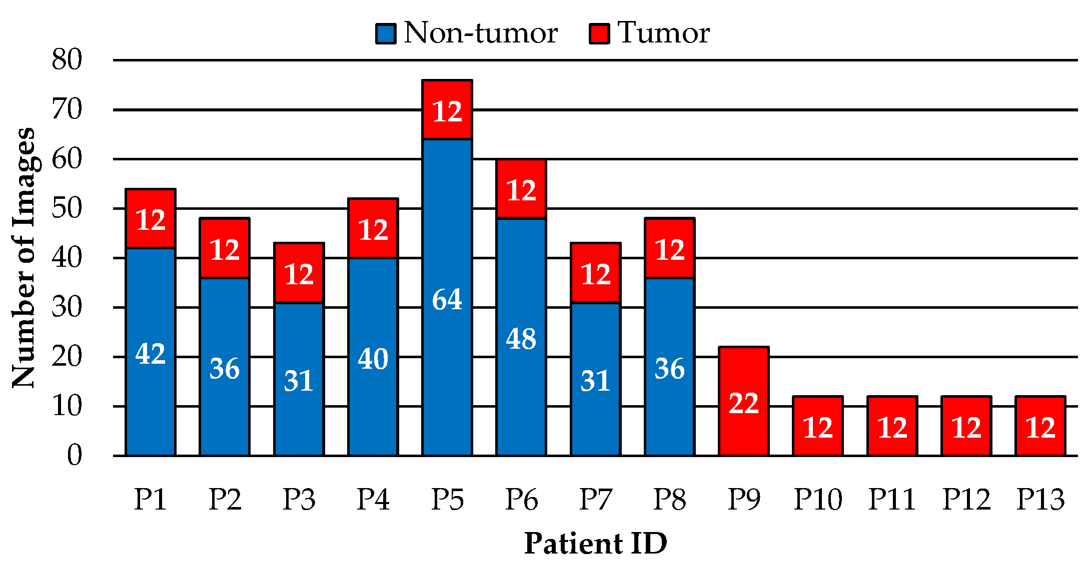
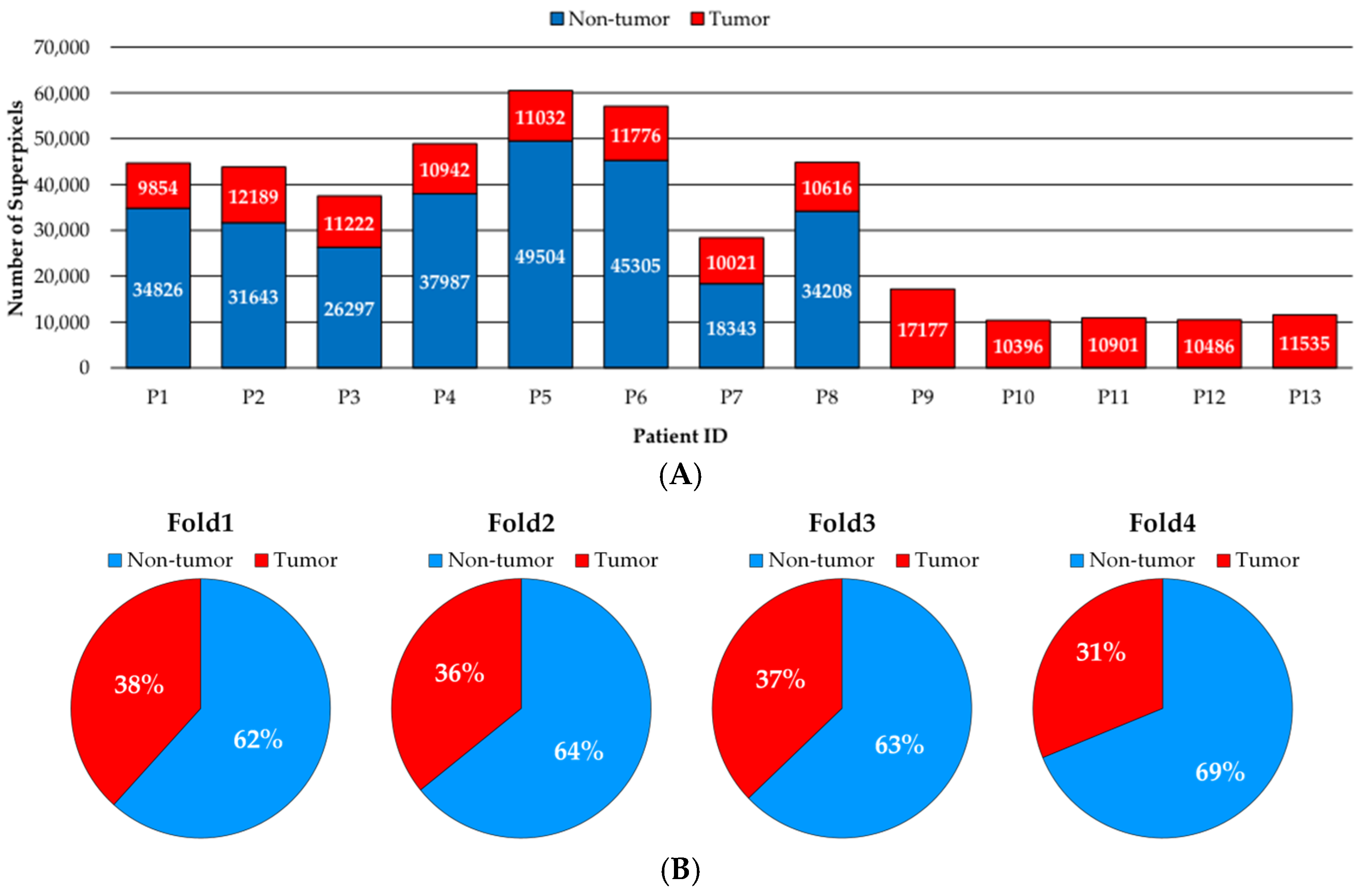
2.1. Dataset Description

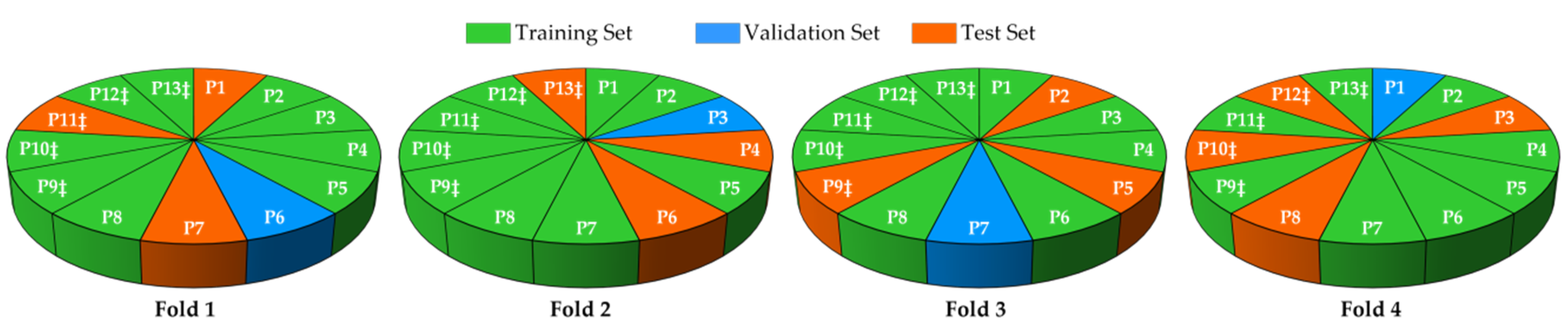
The dataset for this study consisted of a set of HS images acquired from human brain histological slides, as we described earlier [10]. These biological specimens were processed and analyzed by the Pathological Anatomy Department of the University Hospital Doctor Negrín at Las Palmas of Gran Canaria (Spain). The study protocol and consent procedures were approved by the Comité Ético de Investigación Clínica-Comité de Ética en la Investigación (CEIC/CEI) of the same hospital. After histological preparation of the tissue with H&E staining, the samples were examined by pathologists, providing a diagnosis of tissue according to the World Health Organization (WHO) classification of tumors of the nervous system [22]. After the pathologist confirmed the GB diagnosis, macroscopic annotations were made on the physical glass slides with a marker. Non-tumor areas were annotated in blue, while GB areas were annotated in red.

The HS images were captured using a microscope optimized for HS acquisitions equipped with a push-broom camera, which performs spatial scanning for acquisition (Figure 1A). HS image acquisition was performed within the annotated areas of tumor and non-tumor in the slides (Figure 1B). The spectral range of the images was from 400 to 1000 nm with a spectral resolution of 2.8 nm, sampling 826 spectral channels. The camera captures 1004 pixels per line, and the image width was fixed to be 800 pixels. The images were captured using 20 × magnification, producing a HS image size of 375 × 299 µm (Figure 1C). After pre-processing, the HS cubes were formed by 275 spectral channels. Further details about the acquisition system and the data acquisition procedure can be found in [10].

A total of 494 HS images were acquired from 13 slides from 13 different patients with GB. A brief description of the dataset can be seen in Figure 2, which demonstrates that the dataset is not balanced, having more samples from non-tumor tissue than tumor tissue. Additionally, some of the slides only contained tumor tissue, as occurs in patients P9 to P13.

2.2. Data Partition

In order to perform the machine learning analysis, an unbiased data partition should be performed. The dataset used for this study poses three problems. First, the dataset is limited in the number of patients. Second, samples containing both classes (non-tumor and tumor) are only available for eight patients. Hence, the information about the non-tumor samples is limited in terms of patients. Third, the dataset is not balanced, having more images annotated as non-tumor.

For these reasons, the data partition used in this research consists of dividing the data in four different folds, each one built with patient-independent train, validation and test sets (Figure 3). A more comprehensive explanation of the motivations of the proposed data partition is given in [10]. A brief summary of the dataset partition into folds is as follows: (1) data from a single patient is located in training, testing, or validation; (2) validation patients should have both types of annotations (non-tumor and tumor); and (3) all patients have to be included in a test set eventually. The limited total number of patients available leads to a limited number of patients used for validation in each fold. Therefore, it is possible to have overfitting of the models to validation patients.

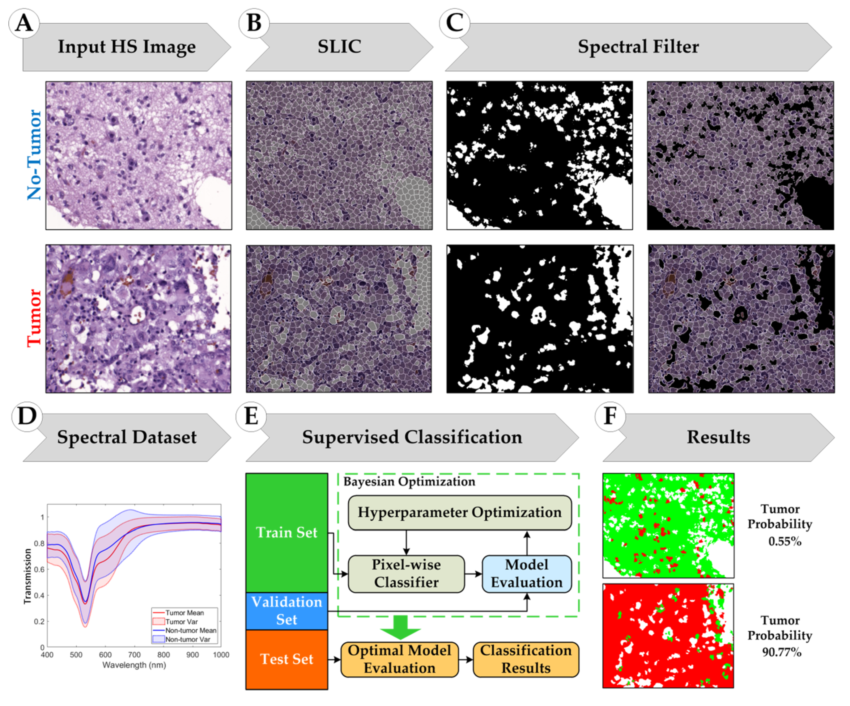
2.3. Superpixel-Based Processing Framework

The proposed processing framework is divided into six steps (Figure 4). First, homogenous spectral areas of the input HS cube (Figure 4A) are extracted by using a superpixel segmentation algorithm (Figure 4B). The main motivation on the use of a superpixel segmentation approach prior to classification is to alleviate the amount of data to be processed, without losing relevant information from the HS image. After superpixel segmentation, superpixels belonging to the background light of the microscope are removed, while superpixels corresponding to tissue are stored (Figure 4C). Since the annotation of the images was performed at a macroscopic level, all the superpixels extracted from a single image are annotated as non-tumor or tumor depending on the annotation of the current image (Figure 4D). Finally, the spectral data from all patients in a fold are used to train, validate and optimize, and test a supervised classifier (Figure 4E). In the test stage, the prediction about the diagnosis of each superpixel (non-tumor or tumor) is performed using the classifier trained and optimized in the training/validation stage. Finally, the classification performance is quantitatively measured, and a representation of the classification is provided as heat and classification maps (Figure 4F).

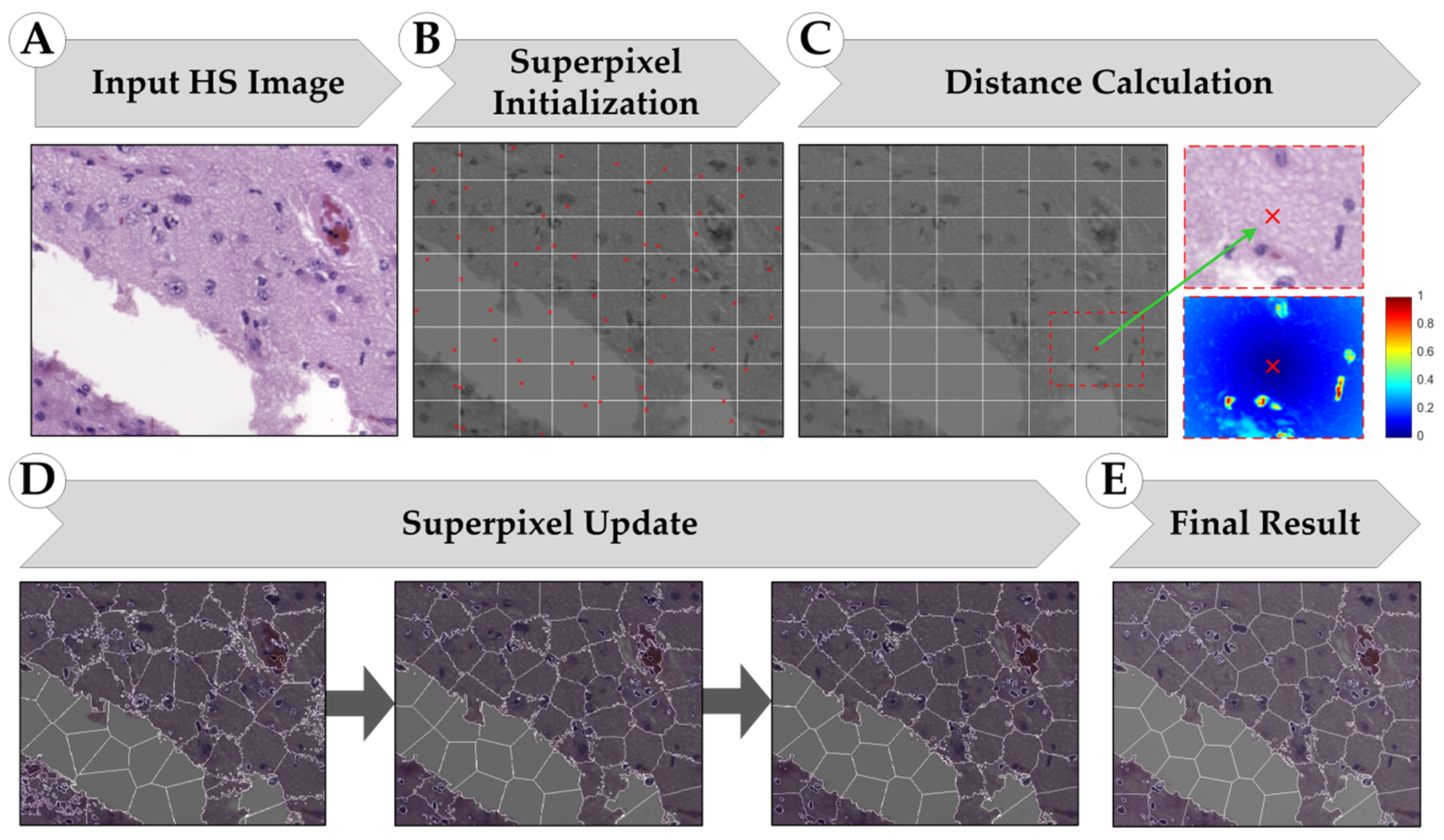
2.3.1. Simple Linear Iterative Clustering (SLIC) Approach

In this research, we used the simple linear iterative clustering (SLIC) superpixel segmentation method proposed by Achanta et al. [12]. This algorithm is a modification of the k-means clustering algorithm to work with superpixels. Given a fixed number of target superpixels ($K$), the SLIC algorithm first initializes the superpixels by dividing the input image (Figure 5A) in a regular grid (Figure 5B). The initial area of the superpixel is $S$ pixels. Next, the initial centroids of each superpixel are assigned to a randomly selected pixel within the superpixel area. Then, for each superpixel centroid, the distance between the superpixel centroid and the pixels in an area of $2·S$ pixels is computed (Figure 5C). After computing this distance for all pixels in the images, each pixel is assigned to a superpixel. Finally, the superpixel centroid is updated (Figure 5D), and the process is repeated until the error in pixel assignment is minimized (Figure 5E).

In the original paper, this approach was developed for conventional RGB images. The distance between a superpixel and a pixel in its neighborhood is calculated as the root mean squared of the color distance and the spatial distance. For each pixel, the color distance ($d_c$) is defined as the Euclidian distance between two color components in the CIELAB color space (a color space defined by the International Commission on Illumination in 1976 [23]), and the spatial distance ($d_S$) is defined as the Euclidean distance between the spatial coordinates of the pixels. In order to compensate for the difference in range between $d_c$ and $d_S$, a hyperparameter $m$ is defined (Equation (1)). This hyperparameter weighs the importance of each type of distance in the overall distance computation. Small values of m make the distance more sensitive to the color distance component, while a large $m$ provides more importance to the spatial component.

$$D_{SLIC}=\sqrt{d_c{}^2+{\left(\frac{d_S}{S}\right)}^2·m^2}$$

(1)

In a first attempt, we utilized the original SLIC algorithm with the HS data. However, in our experiments we found the use of the Euclidian distance for the spectral similarity was not suitable for spectral data. The superpixels generated when using the Euclidian distance were not able to successfully group spectrally similar materials, showing high spectral variations between pixels belonging to the same superpixel. For this reason, we propose some modifications to such distance metrics for adapting SLIC algorithm to HSI. First, we propose the use of the Spectral Angle (SA) as a distance metric for measuring the spectral similarity between two pixels $p_1$ and $p_2$ with $N$ spectral bands (Equation (2)). The use of this type of distance is widely extended in the HSI research community [24]. For the spatial distance, we keep the Euclidian distance between two pixels. The SA distance ($d_{SA}$) is in the range [0,1]. For this reason, in order to compute the total distance ($D_{proposed}$), we propose to simply weight the influence of the spatial distance by multiplying it for a factor $m$ (Equation (3)). This hyperparameter is used to weigh the importance of the spatial and the spectral distance in the superpixel assignment.

$$d_{SA}=\frac{{{\displaystyle \sum }}_{i=1}^N{p}_1{}_i·p_2{}_i}{\sqrt{{{\displaystyle \sum }}_{i=1}^N{p}_1{{}_i}^2}+\sqrt{{{\displaystyle \sum }}_{i=1}^N{p}_2{{}_i}^2}}$$

(2)

$$D_{proposed}=d_{SA}+\left(\frac{d_S}{S}\right)·m$$

(3)

2.3.2. Supervised Classification

The last stage of the superpixel-based processing framework is composed by a supervised classifier employed to perform the classification of each superpixel centroid. Support Vector Machines (SVMs) were employed to perform the experiments since it has been demonstrated in the literature this algorithm performs well with imbalanced datasets [25]. SVMs are supervised classification algorithms widely employed for classification of HS data since they have shown good performance with high dimensional data, even with a limited number of training samples [25]. Vapnik proposed the binary classification approach of the SVM algorithm in 1979 [26]. This algorithm tries to separate two classes ($y_i\in \left\{-1, 1\right\}$) based on the use of a training set composed by $N$ data samples from the d-dimensional feature space ($x_i\in ℝ, \left\{i=1,2,\dots , N\right\}$). The algorithm finds the optimal hyperplane that maximizes the margin defined by a weight vector $w\in ℝ$ and a bias $b\in ℝ$. The prediction of the class of a new data sample is given by equation (4), where $\widehat{y}$ is the predicted class for the data sample $x_i$. The SVM classifier can be used for data which is not linearly separable by using different kernels to map the data in higher dimensional space. In this work, we selected the linear kernel for the SVM approach, employing two different evaluation metrics to optimize the hyperparameter cost (C). This hyperparameter is the constant of constraint violation, which is in charge of deciding if a data sample is classified on the wrong side of the decision limit [27]. MATLAB^® (R2019b, The MathWorks Inc., Natick, MA, USA) was employed to perform the experiments and LIBSVM (Library for Support Vector Machines) was used for the classifier implementation [28].

$$\widehat{y}=x_i·w+b$$

(4)

2.4. Evaluation Metrics

The evaluation metrics employed in this work to assess the performance of the data classification are accuracy (ACC), sensitivity, specificity, precision (PPV), F₁ score (F1) and balanced accuracy (BA). ACC is a metric capable of evaluating overall performance of the classifier by dividing the sum of total number true positives (TP) and true negatives (TN) by the total population of samples (Equation (5)). Sensitivity measures the ability of the classifier to correctly classify the positive samples as presented in Equation (6), where FN is the number of false negatives. On the other hand, specificity measures the ability of the classifier to correctly classify the negative samples as presented in Equation (7), where FP is the number of false positives. BA allows a measurement of the performance of the classifier by balancing the weights of sensitivity and specificity results (Equation (8)). As will be shown later in this work, this metric was necessary to improve the optimization of the hyperparameters of the supervised classifiers. Finally, PPV is the proportion of positive results correctly classified, as expressed in Equation (9), while F1 is the harmonic mean of precision and sensitivity (Equation (10)).

$$ACC=\frac{TN+TP}{TN+TP+FP+FN}$$

(5)

$$Sensitivity=\frac{TP}{TP+FN}$$

(6)

$$Specificity=\frac{TN}{TN+FP}$$

(7)

$$BA=\frac{Sensitivity+Specificity}{2}$$

(8)

$$PPV=\frac{TP}{TP+FP}$$

(9)

$$F1=\frac{2·TP}{2·TP+FP+FN}=2·\frac{PPV·Sensitivity}{PPV+Sensitivity}$$

(10)

3. Experimental Results

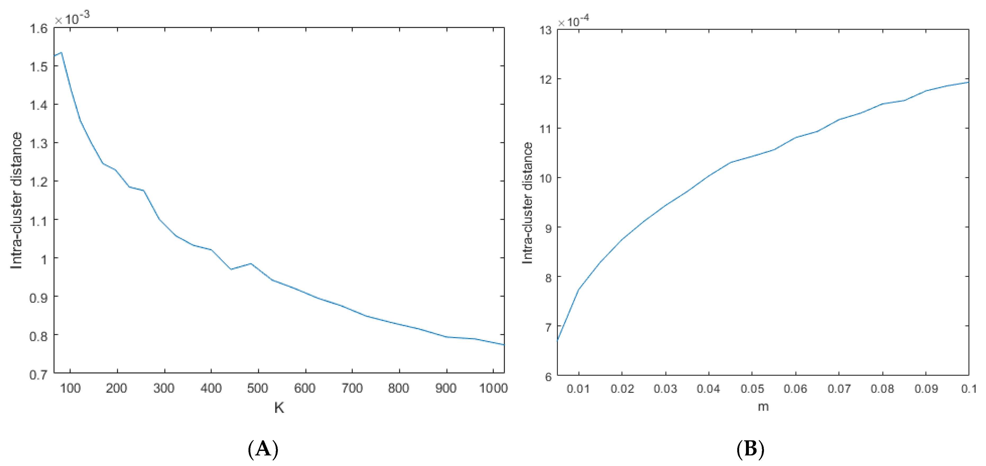
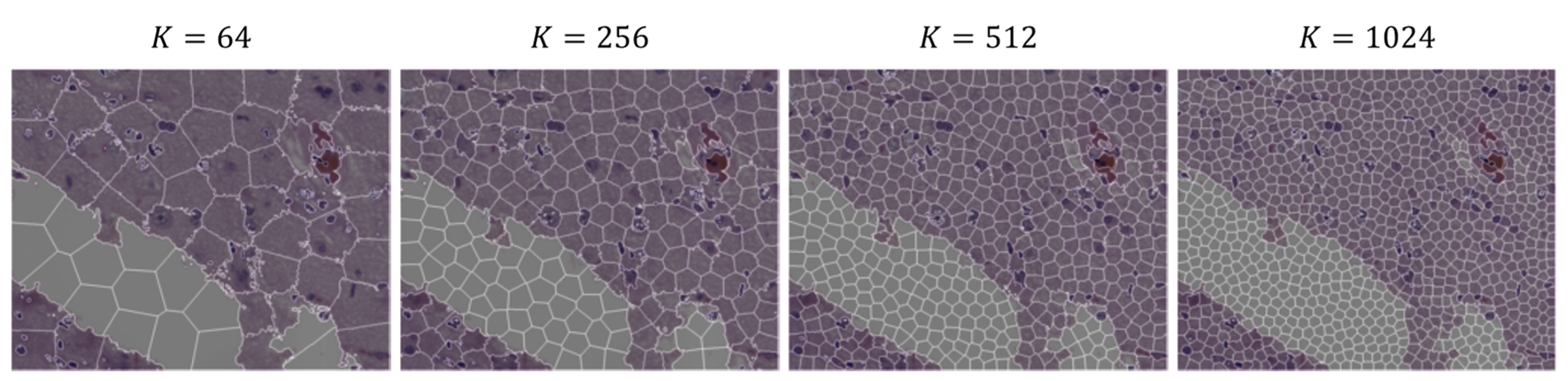
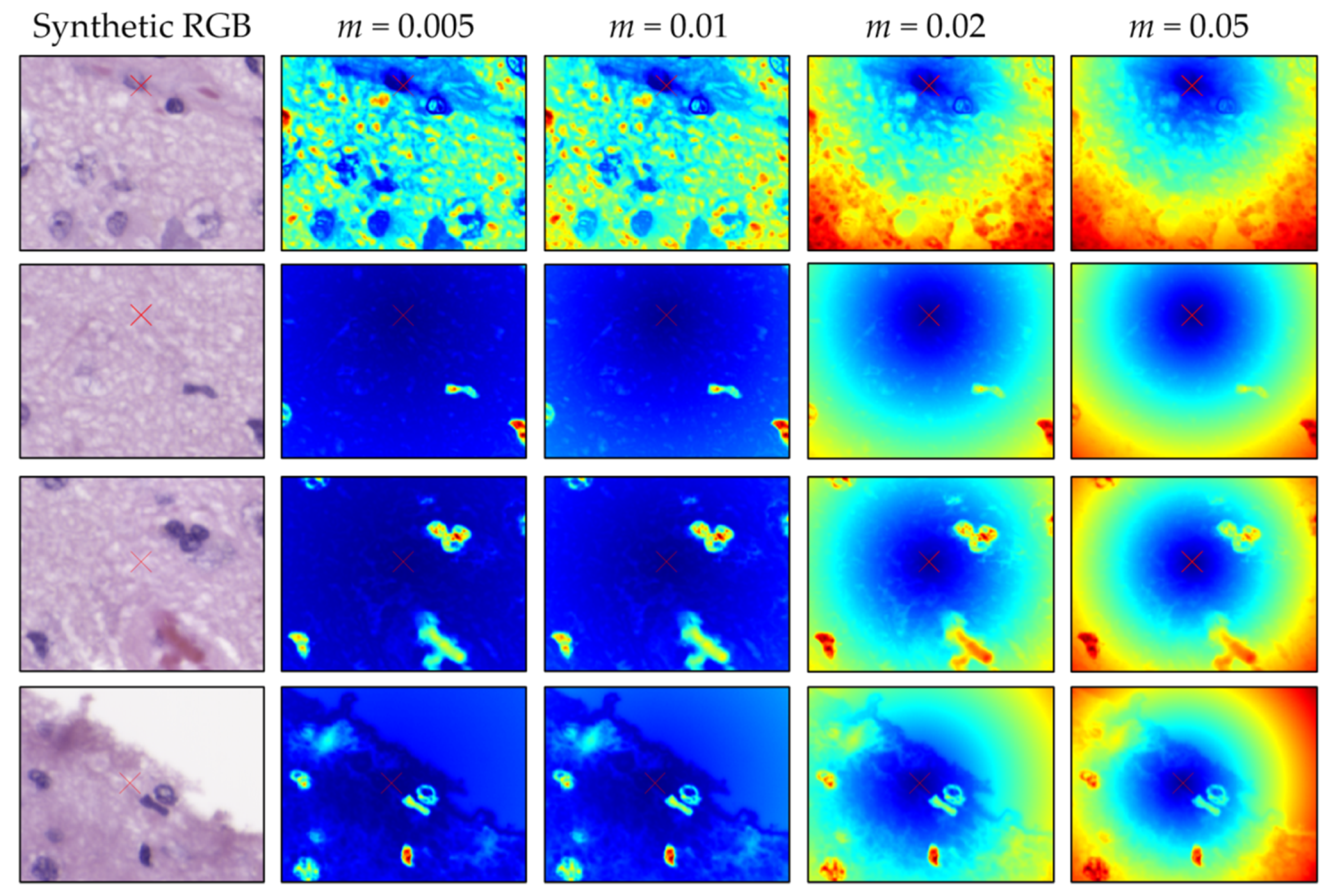
3.1. SLIC Hyperparameter Selection

There are two hyperparameters to be configured on SLIC algorithm: the number of target superpixels ($K$) and the weight parameter ($m$), which balances the contribution of the spectral and the spatial distance. For machine learning, the superpixels will be used as input to a supervised classifier. The main motivation for the use of a superpixel algorithm in the proposed processing framework is to extract the most salient spectral information from each HS image. Therefore, the subsequent superpixel-based classification can be affected if the spectral information within each superpixel does not belong to spectrally consistent areas, i.e., if some superpixels contain pixels with significant different spectral signatures. For this reason, we evaluated the effect of varying both $K$ and $m$ in the mean intra-cluster distance (Equation (11)), where $c_j$ is the centroid of the superpixel $j$, and $x_i$ represents a pixel on the image assigned to such a superpixel. The lower $D_{IC}$, the most similar pixels within a superpixel.

$$D_{IC}=\frac{1}{K}{\displaystyle \sum }_{j=1}^K\frac{1}{N_i}{\displaystyle \sum }_{i=1}^{N_i}{d}_{SA}\left(c_j,x_i\right)+\left(\frac{d_S\left(c_j,x_i\right)}{S}\right)·m$$

(11)

To select the optimal hyperparameters for the SLIC segmentation, we ran the SLIC segmentation with different $K$ and $m$ values and calculated the corresponding intra-cluster distance. We analyzed values of $K$ ranging from 64 to 1024, while the values for $m$ varied from 0.005 to 0.1. In Figure 6, we present the results of these experiments, showing the mean $D_{IC}$ for each hyperparameter.

First, we can observe that with an increased number of superpixels, $K$, the lower inter-cluster distance is achieved. The rationale of this behavior is the following. If the number of superpixels is low, a pixel may be assigned to a superpixel for spatial similarity. On the contrary, if the number of superpixels is high, each superpixel is more likely to reject pixels which are not spectrally similar. For this reason, we selected the maximum value of $K$, 1024.

Second, the value of $m$ equalizes the importance of both the spectral and the spatial distance during the superpixel assignment. Low values of $m$ reduce the importance of the spatial proximity, while prioritizing the importance of the spectral similarity. As can be observed in Figure 6B, the greater values of $m$ result in greater intra-cluster distance. The rationale for this behavior is the following. Large values of $m$ result in the spatial distance outweighing the spectral distance, and superpixels are likely to include pixels that are spatially closer, more than spectrally different. For this reason, we selected a value of $m=0.01$ to provide relevance to the spatial information, while keeping the inter-cluster distance low.

An example of the variation of the SLIC results depending on $K$ is represented on Figure 7. If K is low, the area covered by a single superpixel is high, and could result in a mixture of different elements in a superpixel. As $K$ increases, the area covered by each superpixel decreases, resulting in more compact superpixels. Figure 6 shows that low values of $K$ (64 and 256) produce superpixels that are comprised of pixels from different materials. Additionally, for large values of $K$ (512 and 1024), the superpixels are able to isolate pixels from single materials. In this application, we used the superpixels as a spectral summary of the current HS image. For this reason, the presence of superpixels with heterogenous spectra may lead to inaccurate predictions during supervised classification. In this research, we empirically selected $K=1024$, which was shown to provide spectrally compact areas.

An example of this effect can be observed in Figure 8 for different regions of an image. In this application, we would expect the superpixels to be spectrally coherent. For this reason, we selected $m=0.01$ for the generation of the superpixels.

3.2. Supervised Classification Results

After performing SLIC segmentation in all the images of the dataset, a superpixel dataset was constructed of both tumor and non-tumor annotations. In Figure 9A, we show the distribution of superpixels among the different patients, while Figure 9B represents the distribution of classes between the different folds. In this figure, the imbalanced nature between non-tumor and tumor samples is evident.

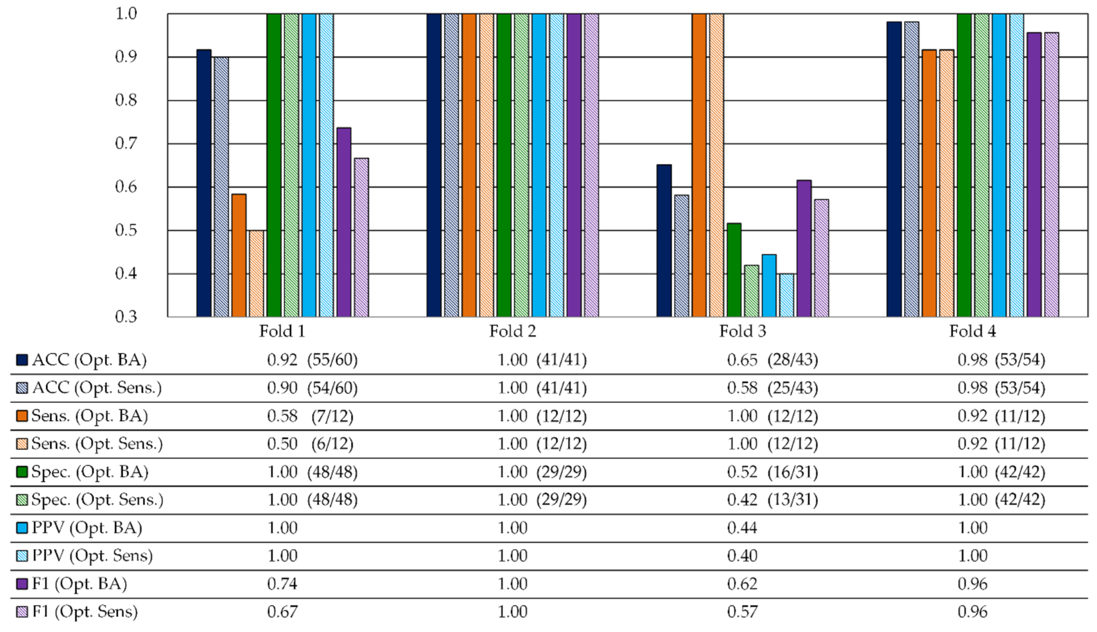
3.2.1. Validation Results

Using the aforementioned superpixel dataset, we used the training data of each fold for training a supervised classifier, and we employed the validation data of each fold to optimize the hyperparameters to increase performance. In this section, we describe the results obtained by using SVMs with linear kernel as classifier. Random Forest and 1-D Convolutional Neural Networks (CNNs) were also evaluated, but the performance of those classifiers was not competitive. For RF we used the MATLAB Machine Learning Toolbox, while 1-D CNN experiments were carried out using the TensorFlow implementation of the Keras Deep Learning API [29,30]. Average validation sensitivity and specificity results of the 1-D CNN classifier were 66.0 ± 31.4% and 60.8 ± 44.2%, respectively. Regarding RF classification, the sensitivity and specificity results were 59.3 ± 43% and 62.3 ± 24%, respectively. Due to the inadequate performance on the validation set, these classifiers were not further evaluated in the subsequent experiments.

In order to tune the hyperparameters of the supervised classifier, the model was trained using the training data, and the performance of the model was evaluated using the validation set. This process was repeated several times by varying the hyperparameters’ values to find the optimal hyperparameters which provided the best performance on the validation set. Finally, the performance of the tuned model was evaluated using the test set.

In this investigation, we performed the classification independently for each fold. Additionally, we proposed several optimization strategies for the hyperparameter optimization. Due to the large number of superpixels in each training fold, the time required to train a linear SVM classifier was about 21 hours. Although this computation time is not prohibitive, the required number of iterations to find the optimal hyperparameter in each fold drastically increased the execution time for finding the optimal classification models. In order to alleviate these training times for each fold, we decided to divide the training data into 10 different data partitions, and then train an ensemble of 10 different SVM classifiers. We first proved there was no performance drop when using the SVM ensemble compared to using all the training data at once. Then, we realized that when using the SVM ensemble the execution time required to train a single fold decreased from 21 hours to 4 hours, which made hyperparameter optimization possible in a reasonable time.

For linear SVM, the cost value was the hyperparameter to be tuned. Instead of performing a grid search of the hyperparameters, we searched the optimal hyperparameters by using a Bayesian optimization algorithm [31]. Due to the imbalanced nature of our dataset, we proposed the use of BA and sensitivity metrics as optimization functions to be minimized. In this case, ACC is not a good metric to be optimized, since it would produce models that are more specialized in detecting the majority class of the dataset. In this optimization framework, the values of cost were bound between ${10}^{-5}$ and ${10}^5$.

Table 1. Superpixel classification results of the validation set in each fold using the SVM with Linear Kernel, with and without hyperparameter optimization.

	No Opt.					Opt. Metric (BA)					Opt. Metric (Sensitivity)
Partition	ACC	Sens.	Spec.	PPV	F1	ACC	Sens.	Spec.	PPV	F1	ACC	Sens.	Spec.	PPV	F1
Fold 1	0.65	0.12	0.78	0.13	0.13	0.88	0.54	0.97	0.84	0.66	0.87	0.47	0.97	0.81	0.60
Fold 2	0.81	0.57	0.91	0.73	0.64	0.95	0.89	0.98	0.96	0.92	0.95	0.88	0.99	0.96	0.92
Fold 3	0.39	0.92	0.10	0.36	0.51	0.61	0.99	0.41	0.48	0.64	0.58	0.99	0.35	0.45	0.62
Fold 4	0.80	0.48	0.89	0.56	0.52	0.89	0.88	0.89	0.69	0.78	0.88	0.89	0.88	0.68	0.77
Avg.	0.66	0.52	0.67	0.44	0.45	0.83	0.82	0.81	0.74	0.75	0.82	0.81	0.80	0.73	0.73
Std.	0.20	0.33	0.39	0.26	0.22	0.15	0.19	0.27	0.21	0.13	0.17	0.23	0.30	0.22	0.15

Sens.: Sensitivity; Spec.: Specificity; Avg.: Average; Std.: Standard Deviation.

shows the final validation results for each fold using the linear kernel with the default cost value ($C=1$) and with the optimal hyperparameters obtained using the BA and the sensitivity metrics. The most relevant outcomes of these results are the following. First, we can see that hyperparameter optimization has a positive impact in the classification results, achieving an increase of 16% (ACC), 29% (sensitivity), 13% (specificity), 29% (PPV), and 28% (F1 metric). Second, the results obtained with optimized models show high accuracy, sensitivity and specificity for Folds 2 and 4 (higher than 88%), while models for Folds 1 and 3 suffer from low sensitivity (47–54%) and low specificity (35–41%), respectively. However, only Fold 1 shows remarkable PPV and F1 results. Finally, the results suggest the hyperparameter selection using BA as the optimization function provides subtly better performance, obtaining an improvement of 1% in the ACC, sensitivity, specificity and PPV metrics and an improvement of 2% in the F1 metric with a reduced standard deviation (std).

As mentioned in the dataset description, the usage of a single patient as validation patient may result in overfitting on the validation patient. We ensure there is no overfitting to the validation data by checking for similar performance between the classification of the training and validation samples within a fold.

In this work, the dataset annotation was performed at a macroscopic level. Therefore, the HS images annotated as tumor would contain some superpixels with spectral features which are not indicative of tumor, such as superpixels that are common in both tumor and non-tumor tissue. These wrong annotations could lead to false positives in the superpixel classification. For this reason, we considered an alternative approach to evaluate the results. Instead of performing the classification over all the superpixels of the validation patient, we also evaluated the image level. To this end, we used the trained SVM model to classify each image from the validation patient. Then, an image is flagged as tumor if more than 50% of the image superpixels are classified as tumor. On the contrary, if fewer than 50%, then the image is flagged as non-tumor. The threshold value of 50% to decide if an image should be flagged as tumor or not was experimentally determined using the validation data. Although it seems 50% is a high value, since intuitively the presence of a few superpixels flagged as tumor may suggest the presence of tumor, this high threshold can be a consequence of the aforementioned incorrectly annotated superpixels. These inappropriate annotations would lead to false positives in the superpixel classification. A graphic representation of this approach is shown on Figure 10.

Results on the validation set using the image classification approach are shown in Figure 11. These results were obtained from the SVM model optimized using BA and sensitivity. On the one hand, similarly to the previous evaluation, Folds 2 and 4 present the best performance. In Fold 2, all the images are correctly classified. For Fold 4, only a single non-tumor image and one tumor image are misclassified. For these folds, the performance of both types of SVM models work similarly. On the other hand, the classification performance for Folds 3 and 4 is lower. In Fold 1, the sensitivity is low, and several images from tumor samples are not flagged as tumor, but all the images from non-tumor class are correctly classified. In opposition, in Fold 3 all tumor images are correctly classified, but one half of the non-tumor images are misclassified.

Regarding the comparison about the type of optimization for hyperparameter selection, the performance of the SVM optimized by BA is subtly higher compared to optimization driven by sensitivity.

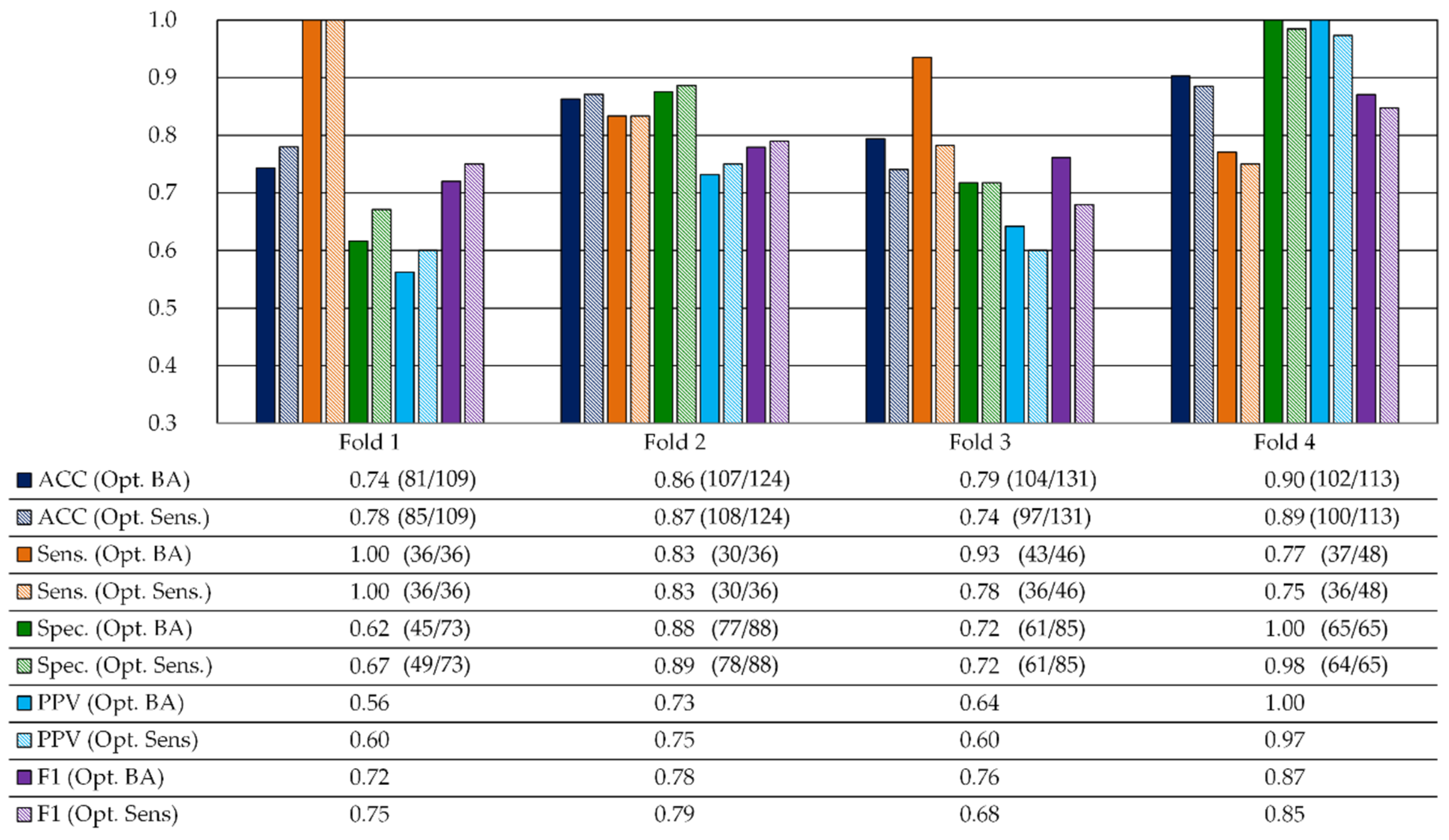
3.2.2. Quantitative Test Results

In this section, we show the classification results for the test set of each fold. The quantitative results obtained for the test set for the SVM Linear classifier optimized with the BA and the sensitivity metrics are shown in Figure 12. On average, the use of the BA metric for the hyperparameter optimization provided better ACC results (82.6 ± 7.1%) than the Sensitivity metric (78.3 ± 6.2%). Considering sensitivity and specificity results, the classifier optimized with the BA metric provided a result of 88.5 ± 10.2% and 80.2 ± 16.9%, respectively, representing an improvement in the sensitivity of 4.3% with respect to the classifier optimized with the sensitivity metric. Regarding the differences between the use of BA metric and sensitivity metric in the PPV and F1 results, PPV were practically the same, achieving 73.4 ± 19% and 73.1 ± 17.6%, respectively, while F1 improved 1.6% using the BA metric (78.3 ± 6.4%). For this reason, the BA metric was shown as a suitable evaluation metric to optimize the hyperparameters of a supervised classifier with imbalanced datasets for this specific application.

Finally, in Figure 13, we show the results obtained of each patient individually. For every patient except for P2, P6, P8 and P10, the sensitivity is higher than 90%. For P2 and P8, the sensitivity is also high, beyond 80%. For P6 and P10, the sensitivity is low. These patients were classified using models from Folds 2 and 4, respectively. However, models from those folds demonstrated good sensitivity for the remaining patients. This fact will be further investigated in future works. The specificity can only be measured for patients with both types of annotations (non-tumor and tumor), i.e., from P1 to P8. Five of these patients present a sensitivity of 100%, while the others present low specificity. The worst case is P7, where the specificity is 10%.

The high sensitivity of the proposed methodology suggests that it could serve as a clinical tool to detect images with suspicious tumor presence for a pathologist to examine. However, despite the fact that the overall amount of time spent in examination could be reduced, the low specificity would likely result in some false positives.

Table 2. Results comparison between the proposed superpixel-based approach and a previous work using a CNN-based approach [10].

	Proposed Superpixel-Based Approach (Results at Image Level)			Proposed Superpixel-Based Approach (Results at Superpixel Level)			Previous CNN-Based Approach [10] (Results at Patch Level)
Partition	ACC	Sensitivity	Specificity	ACC	Sensitivity	Specificity	ACC	Sensitivity	Specificity
P1	1.00	1.00	1.00	0.91	0.91	0.90	0.93	0.91	0.96
P2	0.94	0.83	1.00	0.79	0.50	0.97	0.89	0.99	0.83
P3	1.00	1.00	1.00	0.90	0.88	0.92	0.85	0.91	0.8
P4	0.79	1.00	0.73	0.78	0.87	0.75	0.57	0.57	0.58
P5	0.68	1.00	0.63	0.54	0.67	0.51	0.69	0.81	0.64
P6 *	0.90	0.50	1.00	0.85	0.35	0.98	-	-	-
P7	0.35	1.00	0.10	0.53	0.95	0.30	0.66	0.71	0.63
P8	0.96	0.83	1.00	0.89	0.75	0.93	0.96	0.96	0.96
P9	0.95	0.95	-	0.92	0.92	-	0.99	0.99	-
P10	0.25	0.25	-	0.41	0.41	-	0.89	0.89	-
P11	1.00	1.00	-	0.98	0.98	-	0.92	0.92	-
P12	1.00	1.00	-	0.83	0.83	-	0.92	0.92	-
P13	1.00	1.00	-	0.97	0.97	-	0.99	0.99	-
Avg.	0.83	0.91	0.78	0.79	0.80	0.76	0.86	0.88	0.77
Std.	0.27	0.22	0.34	0.19	0.19	0.26	0.14	0.13	0.16

* Data not available for CNN-based approach and excluded for the computation of the average (Avg.) and standard deviation (Std.) values.

shows the results of the proposed superpixel approach (reporting both the results at image and superpixel level) and the previous work, where the same data were classified using a patch-based CNN approach (reporting the results at patch level) [10]. As shown in Table 2, data from P6 are missing from the CNN experiments. In our previous work, we found an error in the annotations of P6, and this patient was removed from the dataset. In this study, we corrected the annotation errors of this patient. However, to provide a fair comparison between the two different processing approaches, P6 patient has not been included in the computation of the mean metrics. The average ACC results obtained with the proposed approach (considering the results at image level) is 3% below the CNN-based approach. However, the average sensitivity obtained with the superpixel-based approach is higher than the CNN results, 91% and 88%, respectively. Moreover, the average specificity is slightly improved using the proposed approach (78%) with respect to the CNN-based approach (77%). Considering the fact that the superpixel approach only exploits spectral information, the results achieved in this preliminary study are competitive with respect to the CNN approach, which uses both spatial and spectral properties. Moreover, it is worth noting that the amount of data generated with the patch-based CNN approach is extremely large (49,565 image patches of 87 × 87 pixels with 275 bands, i.e., approx. 768 Gigabytes) compared to the data generated for the superpixel-based approach (426,260 superpixels with 275 bands, i.e., approx. 0.87 Gigabytes). Hence, the CNN approach requires substantial memory and computational requirements to perform the classification of the data, while the superpixel-based approach alleviates these requirements. This is especially important when targeting real-time aid visualization tools for histological screening process during clinical routine practice with the goal of assisting pathologist during diagnostic procedures.

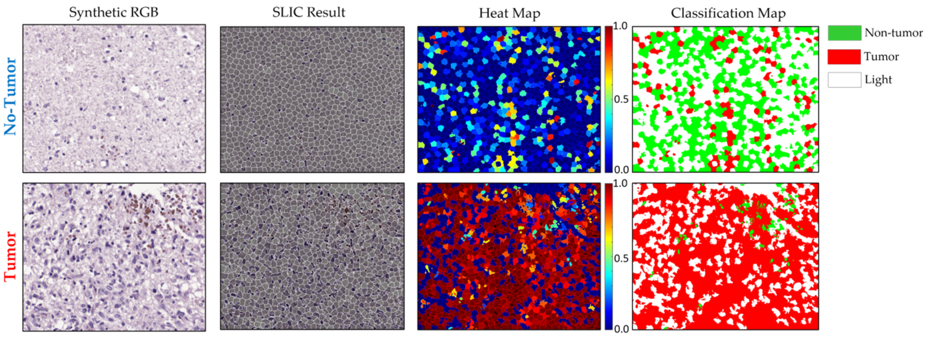
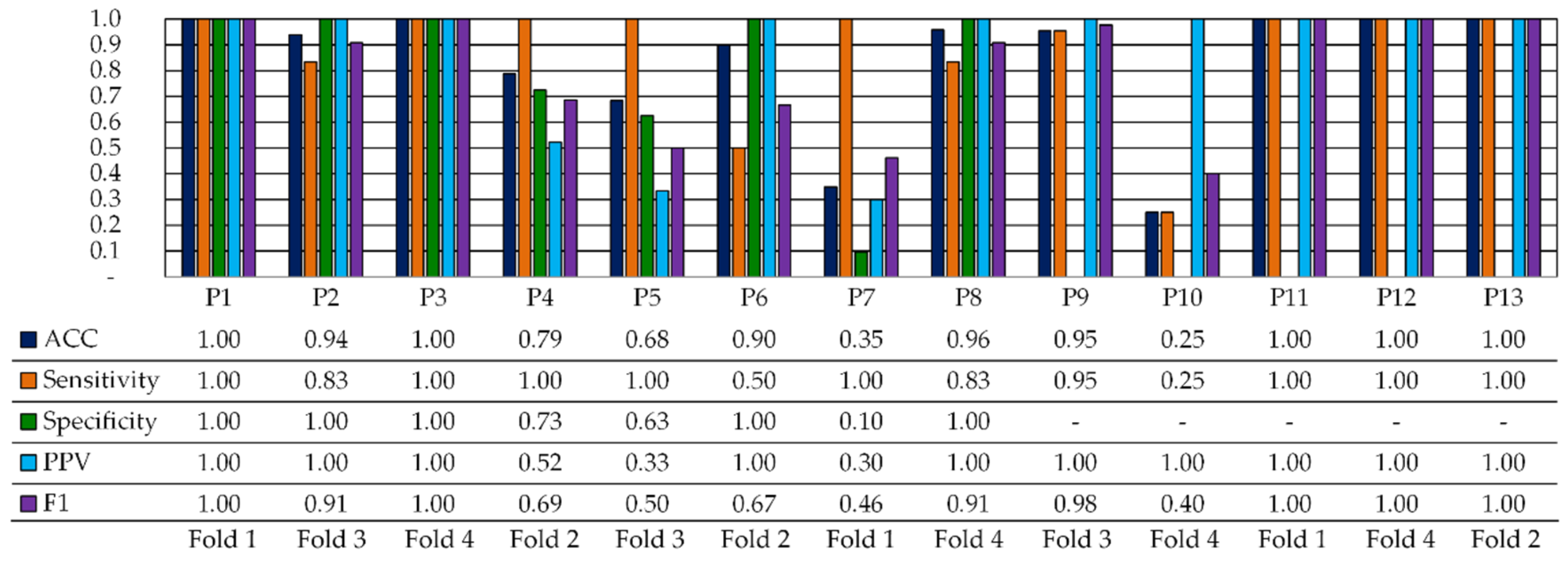
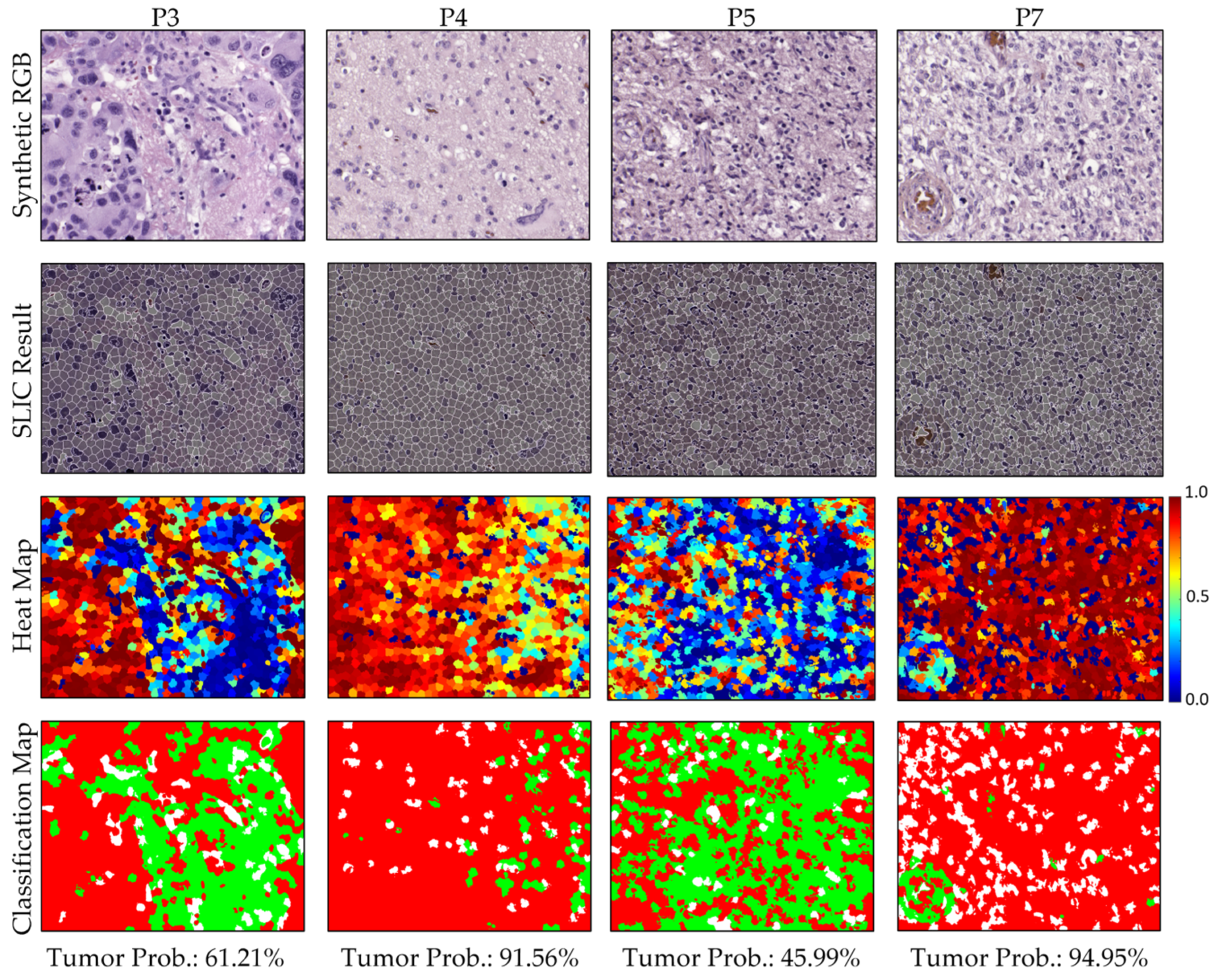
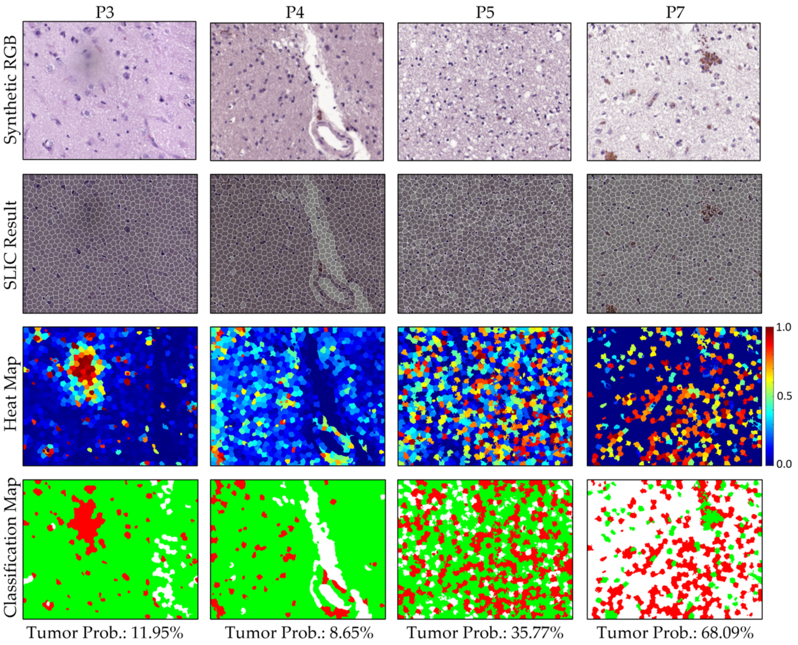
3.2.3. Qualitative Test Results

The results of the proposed approach can be visualized as a heat map, which shows the predicted tumor probability map of superpixels, or as a classification map, where the superpixels are assigned to a class using a probability threshold of 50%.

Figure 14 shows four examples of qualitative results obtained from four tumor images, belonging to P3, P4, P5, and P7, with their respective tumor presence probability. For P3, 61% of the superpixels were classified as tumor, thus the image-scale prediction is tumor. The heat maps for P4 and P7 suggest the presence of tumor with high probability. On the contrary, the heat map for P5 shows a misclassification, where about 46% of the superpixels were classified as tumor, so the image is misclassified, being a false negative prediction.

Figure 15 shows the results of four example non-tumor images that belong to P3, P4, P5, and P7 with their respective tumor probability results. As can be seen, the heat maps for P3, P4 and P5 show a successful classification of non-tumor samples. For P3 and P4, only a few superpixels were classified as tumor, less than 13% of the image in either case. In the case of P5, the image was flagged as non-tumor, but the number of superpixels classified as tumor is higher, about 36%. Finally, we show an example of a false positive, where 68% of the superpixels were classified as tumor and thus the image was flagged as tumor.

As mentioned previously, the presence of misannotated superpixels in the dataset could lead in misclassifications. For this reason, we selected the 50% tumor threshold. Although in most situations this strategy provides an accurate diagnosis, there are some limitations. For example, in Figure 14, we can observe how the image belonging to P5 was misclassified as a non-tumor image, while the number of superpixels classified as tumor was around 46%. On the contrary, the image from P7 in Figure 15 represents a false positive because around 68% of the superpixels were classified as tumor. However, this behavior is only found in a few examples of the dataset.

4. Discussion

The main limitation of this study is the reduced number of patients and the imbalance of the dataset. Additionally, only 8 out of the 13 patients have annotated data available from the two classes, i.e., tumor and non-tumor. This fact, together with the known histological heterogeneity of GB tumors, makes this task very challenging. Therefore, more patients are needed in future analysis to obtain more robust conclusions about the ability of HSI and ML for the automatic detection of GB in histological slides. More concretely, to obtain statistically significant results, we hypothesize that at least 10 patients are needed with both types of annotations for both validation and test. This would require at least 40 patients with both types of annotations to train the classifiers. The main challenges for the acquisition of such a dataset are the large amounts of data generated during image acquisition and the time-consuming manual annotation for the ground truth. Further data acquisition campaigns will be deployed to increase our dataset, reinforcing the conclusions achieved in this work about the potential use of the HS superpixel-based approach to detect GB in histological slides. Regarding the imbalanced dataset, in this manuscript we deal with this problem by using a hyperparameter optimization guided by metrics which may compensate the data imbalance, i.e., balanced accuracy and sensitivity. The use of sensitivity was motivated by the lower number of examples in the tumor class (~35% of tumor superpixels, compared to ~65% of non-tumor superpixels). Nevertheless, other metrics can be used to drive the hyperparameter optimization to alleviate the effect of the imbalanced dataset. For example, the F-1 score or a weight balance between precision and recall, where the weight will favor the class with lower number of samples.

Future studies will address some limitations of this work. First, in this work, the images were collected in a laboratory environment under controlled conditions. One of the main challenges associated to medical imaging processing is dealing with noisy images. Although in this work we focused in investigating the potential of HS images for the identification of tumor, in future works we will further analyze the effect of noise removal strategies in both the superpixel and the classification approaches [32,33,34]. Second, as previously mentioned, due to the macroscopic annotations, some regions of the tumor HS images are in fact not characteristic of GB tumor, but are still labeled as tumor. Such misannotated data are likely to produce superpixel misclassifications. To handle this fact, one of the future works in this field will be to identify which superpixel spectra can be found in both tumor and non-tumor images, which may improve the quality of the predictions. Third, although the spatial information of the HS is partially considered when the superpixels are extracted with SLIC, the supervised classification is only focused on the spectral information. In this study, we demonstrated the potential of the exclusive use of spectral information for the identification of tumor areas in HS digitized slides. Nevertheless, these results can be further improved if we also include additional spatial information into the classification framework. For example, as shown in the work by Zhao et al. [35], it could be possible to develop a method which efficiently combines the spectral information from the proposed superpixel approach with the spatial information extracted from the HS data using a 2D-CNN. Another challenge to be addressed in future works is to improve the way the optimal number of superpixels is extracted. In this research, we selected the number of superpixels to minimize the intra-cluster distance, but more sophisticated methods can be used in the future to reduce the number of superpixels while retaining the most important information from each image [36]. In this research, we overestimated the number of superpixel centroids in order to ensure proper extraction of spectral features from the HS image. However, the computational time could be reduced by decreasing the number of superpixels per image, which is more competitive for screening histology slides.

Finally, regarding the supervised classification, after testing SVM, 1-D CNN, and RF algorithms, the only classifier that demonstrated accurate classification results in our data was SVM. All of these classifiers have demonstrated high performance with spectral data in the literature [10]. However, the classification performance strongly depends on the data used to train the model. Although those classifiers did not perform well in our application, we cannot suggest that using a larger dataset would allow those classifiers to correctly classify the spectral data. Moreover, it is possible that the 1-D CNN underperformed because of the nature of the task. Specifically, the HS signatures were 1-D signals averaged from across a superpixel. The strengths of CNN methods are typically learning from highly variable data with spatial features.

In this work, we only explored the linear kernel of the SVM to demonstrate the feasibility of the superpixel-based approach exploiting only the spectral information. However, in future works, we will evaluate the performance of different kernels for this task with the goal of trying to improve the classification results obtained in this preliminary work.

5. Conclusions

In this work, we propose a combination of superpixel segmentation and supervised classification for the identification of GB tumor in HS images from brain histological slides. First, we modified and optimized the original SLIC segmentation algorithm for HS images. These modifications included the use of a spectral distance based on the spectral angle, and the modification of the global distance, which is a tradeoff between the spectral and the spatial distances between pixels in a neighborhood. After optimizing the hyperparameters of the SLIC algorithm to generate compact pixels, the superpixels were used to build a dataset where superpixels were labeled as tumor or non-tumor according to the pathologists’ annotations. The data were then partitioned in patient-independent training, validation, and test sets. Finally, superpixels were classified using a linear SVM classifier.

The results obtained with this methodology are promising, showing high sensitivity and specificity values for almost all the patients independently. On average, our proposed approach achieved 87% and 81% of sensitivity and specificity, respectively. Additionally, 8 out of the 13 patients obtained a sensitivity of 100%, and 3 out of the 13 had a sensitivity of 83–95%. Screening tests with high sensitivities could be useful clinically. The outcomes of this processing framework could potentially be used in a clinical application to flag which regions of the histological slide are of interest to be further analyzed by a pathologist, and then reduce whole-slide examination.

References

1. Van Es, S.L. Digital pathology: Semper ad meliora. Pathology 2019, 51, 1–10. [Google Scholar] [CrossRef]
2. Halicek, M.; Fabelo, H.; Ortega, S.; Callico, G.M.; Fei, B. In-Vivo and Ex-Vivo Tissue Analysis through Hyperspectral Imaging Techniques: Revealing the Invisible Features of Cancer. Cancers (Basel) 2019, 11, 756. [Google Scholar] [CrossRef] [PubMed] [Green Version]
3. Akbari, H.; Halig, L.V.; Schuster, D.M.; Osunkoya, A.; Master, V.; Nieh, P.T.; Chen, G.Z.; Fei, B. Hyperspectral imaging and quantitative analysis for prostate cancer detection. J. Biomed. Opt. 2012, 17, 0760051. [Google Scholar] [CrossRef] [PubMed]
4. Awan, R.; Al-Maadeed, S.; Al-Saady, R. Using spectral imaging for the analysis of abnormalities for colorectal cancer: When is it helpful? PLoS ONE 2018, 13, e0197431. [Google Scholar] [CrossRef]
5. Septiana, L.; Suzuki, H.; Ishikawa, M.; Obi, T.; Kobayashi, N.; Ohyama, N.; Ichimura, T.; Sasaki, A.; Wihardjo, E.; Andiani, D. Elastic and collagen fibers discriminant analysis using H&E stained hyperspectral images. Opt. Rev. 2019, 26, 369–379. [Google Scholar]
6. Khelifi, R.; Adel, M.; Bourennane, S. Multispectral texture characterization: Application to computer aided diagnosis on prostatic tissue images. EURASIP J. Adv. Signal Process. 2012, 2012, 118. [Google Scholar] [CrossRef] [Green Version]
7. Wang, Q.; Wang, J.; Zhou, M.; Li, Q.; Wang, Y.; Ang, Q.I.A.N.W.; Ang, J.I.W.; Hou, M.E.I.Z.; Ingli, Q.L.I.; Iting, Y.; et al. Spectral-spatial feature-based neural network method for acute lymphoblastic leukemia cell identification via microscopic hyperspectral imaging technology. Biomed. Opt. Express 2017, 8, 3017–3028. [Google Scholar] [CrossRef] [PubMed] [Green Version]
8. Haj-Hassan, H.; Chaddad, A.; Harkouss, Y.; Desrosiers, C.; Toews, M.; Tanougast, C. Classifications of multispectral colorectal cancer tissues using convolution neural network. J. Pathol. Inform. 2017, 8, 1. [Google Scholar]
9. Malon, C.; Cosatto, E. Classification of mitotic figures with convolutional neural networks and seeded blob features. J. Pathol. Inform. 2013, 4, 9. [Google Scholar] [CrossRef]
10. Ortega, S.; Halicek, M.; Fabelo, H.; Camacho, R.; Plaza, M.D.L.L.; Godtliebsen, F.; Callicó, G.M.; Fei, B. Hyperspectral Imaging for the Detection of Glioblastoma Tumor Cells in H&E Slides Using Convolutional Neural Networks. Sensors 2020, 20, 1911. [Google Scholar]
11. Yu, H.; Yang, Z.; Tan, L.; Wang, Y.; Sun, W.; Sun, M.; Tang, Y. Methods and datasets on semantic segmentation: A review. Neurocomputing 2018, 304, 82–103. [Google Scholar] [CrossRef]
12. Achanta, R.; Shaji, A.; Smith, K.; Lucchi, A.; Fua, P.; Süsstrunk, S. SLIC Superpixels Compared to State-of-the-Art Superpixel Methods. IEEE Trans. Pattern Anal. Mach. Intell. 2012, 34, 2274–2282. [Google Scholar] [CrossRef] [PubMed] [Green Version]
13. Zhang, Y.; Liu, K.; Dong, Y.; Wu, K.; Hu, X. Semisupervised Classification Based on SLIC Segmentation for Hyperspectral Image. In IEEE Geoscience and Remote Sensing Letters; IEEE: Piscataway, NJ, USA, 2019; pp. 1–5. [Google Scholar]
14. Zu, B.; Xia, K.; Li, T.; He, Z.; Li, Y.; Hou, J.; Du, W. SLIC Superpixel-Based l2,1-Norm Robust Principal Component Analysis for Hyperspectral Image Classification. Sensors 2019, 19, 479. [Google Scholar] [CrossRef] [PubMed] [Green Version]
15. Tang, Y.; Zhao, L.; Ren, L. Different Versions of Entropy Rate Superpixel Segmentation For Hyperspectral Image. In Proceedings of the 2019 IEEE 4th International Conference on Signal and Image Processing (ICSIP), Wuxi, China, 19–21 July 2019; pp. 1050–1054. [Google Scholar]
16. Xie, F.; Lei, C.; Jin, C.; An, N. A Novel Spectral–Spatial Classification Method for Hyperspectral Image at Superpixel Level. Appl. Sci. 2020, 10, 463. [Google Scholar] [CrossRef] [Green Version]
17. Alkhatib, M.Q.; Velez-Reyes, M. Improved Spatial-Spectral Superpixel Hyperspectral Unmixing. Remote Sens. 2019, 11, 2374. [Google Scholar] [CrossRef] [Green Version]
18. Chung, H.; Lu, G.; Tian, Z.; Wang, D.; Chen, Z.G.; Fei, B. Superpixel-Based Spectral Classification for the Detection of Head and Neck Cancer with Hyperspectral Imaging. In Proceedings of the SPIE Medical Imaging, San Diego, CA, USA, 27 February–03 March 2016; Gimi, B., Krol, A., Eds.; SPIE: Bellingham, WA, USA, 2016; Volume 9788, p. 978813. [Google Scholar]
19. Bejnordi, B.E.; Litjens, G.; Hermsen, M.; Karssemeijer, N.; van der Laak, J.A.W.M. A Multi-Scale Superpixel Classification Approach to the Detection of Regions of Interest in Whole Slide Histopathology Images. In Proceedings of the SPIE Medical Imaging, Orlando, Florida, USA, 21–26 February 2015; Gurcan, M.N., Madabhushi, A., Eds.; SPIE: Bellingham, WA, USA, 2015; Volume 9420, p. 94200H. [Google Scholar]
20. Turkki, R.; Linder, N.; Kovanen, P.; Pellinen, T.; Lundin, J. Antibody-supervised deep learning for quantification of tumor-infiltrating immune cells in hematoxylin and eosin stained breast cancer samples. J. Pathol. Inform. 2016, 7, 38. [Google Scholar] [CrossRef] [PubMed]
21. Zormpas-Petridis, K.; Failmezger, H.; Raza, S.E.A.; Roxanis, I.; Jamin, Y.; Yuan, Y. Superpixel-Based Conditional Random Fields (SuperCRF): Incorporating Global and Local Context for Enhanced Deep Learning in Melanoma Histopathology. Front. Oncol. 2019, 9, 1045. [Google Scholar] [CrossRef]
22. Louis, D.N.; Perry, A.; Reifenberger, G.; Von Deimling, A.; Figarella, D.; Webster, B.; Hiroko, K.C.; Wiestler, O.D.; Kleihues, P.; Ellison, D.W.; et al. The 2016 World Health Organization Classification of Tumors of the Central Nervous System: A summary; Springer: Berlin/Heidelberg, Germany, 2016; Volume 131, pp. 803–820. [Google Scholar]
23. Carter, E.C.; Schanda, J.D.; Hirschler, R.; Jost, S.; Luo, M.R.; Melgosa, M.; Ohno, Y.; Pointer, M.R.; Rich, D.C.; Vienot, F.; et al. CIE 015:2018 Colorimetry, 4th ed.; Technical Report; International Commission on Illumination: Vienna, Austria, 2018. [Google Scholar]
24. Van der Meer, F. The effectiveness of spectral similarity measures for the analysis of hyperspectral imagery. Int. J. Appl. Earth Obs. Geoinf. 2006, 8, 3–17. [Google Scholar] [CrossRef]
25. Ghamisi, P.; Plaza, J.; Chen, Y.; Li, J.; Plaza, A.J. Advanced Spectral Classifiers for Hyperspectral Images: A review. IEEE Geosci. Remote Sens. Mag. 2017, 5, 8–32. [Google Scholar] [CrossRef] [Green Version]
26. Vapnik, V. Support vector machine. Mach. Learn. 1995, 20, 273–297. [Google Scholar]
27. Mercier, G.; Lennon, M. Support Vector Machines for Hyperspectral Image Classification with Spectral-based kernels. In Proceedings of the International Geoscience and Remote Sensing Symposium (IGARSS), Toulouse, France, 21–25 July 2003; Volume 1, pp. 288–290. [Google Scholar]
28. Chang, C.-C.; Lin, C.-J. LIBSVM: A library for support vector machines. ACM Trans. Intell. Syst. Technol. 2011, 2, 27. [Google Scholar] [CrossRef]
29. Abadi, M.; Agarwal, A.; Barham, P.; Brevdo, E.; Chen, Z.; Citro, C.; Corrado, G.S.; Davis, A.; Dean, J.; Devin, M.; et al. TensorFlow: Large-Scale Machine Learning on Heterogeneous Distributed Systems. arXiv 2016, arXiv:1603.04467. [Google Scholar]
30. Chollet, F. Keras. Available online: https://keras.io (accessed on 28 October 2019).
31. Snoek, J.; Larochelle, H.; Adams, R.P. Practical Bayesian Optimization of Machine Learning Algorithms. arXiv 2012, arXiv:1206.2944. [Google Scholar]
32. Saulig, N.; Lerga, J.; Milanovic, Z.; Ioana, C. Extraction of Useful Information Content From Noisy Signals Based on Structural Affinity of Clustered TFDs’ Coefficients. IEEE Trans. Signal Process. 2019, 67, 3154–3167. [Google Scholar] [CrossRef]
33. Hržić, F.; Štajduhar, I.; Tschauner, S.; Sorantin, E.; Lerga, J. Local-Entropy Based Approach for X-Ray Image Segmentation and Fracture Detection. Entropy 2019, 21, 338. [Google Scholar] [CrossRef] [Green Version]
34. Mandić, I.; Peić, H.; Lerga, J.; Štajduhar, I. Denoising of X-ray Images Using the Adaptive Algorithm Based on the LPA-RICI Algorithm. J. Imaging 2018, 4, 34. [Google Scholar] [CrossRef] [Green Version]
35. Zhao, W.; Du, S. Spectral-Spatial Feature Extraction for Hyperspectral Image Classification: A Dimension Reduction and Deep Learning Approach. IEEE Trans. Geosci. Remote Sens. 2016, 54, 4544–4554. [Google Scholar] [CrossRef]
36. Patil, C.; Baidari, I. Estimating the Optimal Number of Clusters k in a Dataset Using Data Depth. Data Sci. Eng. 2019, 4, 132–140. [Google Scholar] [CrossRef] [Green Version]
Figure 1. HS data acquisition procedure. (A) HS microscope-based acquisition system. (B) Pathological slide with macroscopic diagnosis annotations. Yellow squares represent an example of the captured areas for tumor and non-tumor HS images. (C) Examples of non-tumor and tumor HS images acquired at 20×.
Applsci 10 04448 g001
Figure 2. Number of non-tumor and tumor HS images per patient.
Applsci 10 04448 g002
Figure 3. Data partition among the different folds (patients with only tumor samples are marked with ‡).
Applsci 10 04448 g003
Figure 4. Proposed superpixel-based hyperspectral image processing framework.
Applsci 10 04448 g004
Figure 5. Block diagram of the different steps of the SLIC approach for superpixel classification.
Applsci 10 04448 g005
Figure 6. Different SLIC Intra-cluster distance for different SLIC hyperparameters: (A) K and (B) m .
Applsci 10 04448 g006
Figure 7. Different SLIC segmentation results depending on the number of target superpixels (K).
Applsci 10 04448 g007
Figure 8. Different SLIC segmentation results depending on the distant hyperparameter (m). The rows present different image area example around a superpixel centroid (red cross). The first column shows the synthetic RGB image of the area and the remaining columns shows the distance between the superpixel centroid and the rest of pixels in the area with different values of m.
Applsci 10 04448 g008
Figure 9. Number of non-tumor and tumor superpixels per patient (A) and percentage of the total per fold (B).
Applsci 10 04448 g009
Figure 10. Classification results of the majority voting of superpixels classified by SVM. The top row shows a representative non-tumor image RGB composite and its corresponding SLIC result (left), the corresponding superpixel heat map and the binarized form of tumor and non-tumor superpixels (right), where the white color represent the superpixels that correspond with light, green and red colors represent the non-tumor and tumor superpixels, respectively. The result contains less than 50% tumor superpixels, so it is classified as non-tumor. The bottom row shows of a tumor image, where it is possible to observe that the result contains higher than 50% tumor superpixels, so this image is classified as tumor.
Applsci 10 04448 g010
Figure 11. Average image classification results of each fold in the validation set using both metrics (BA and Sensitivity) for the hyperparameter optimization of the SVM Linear kernel.
Applsci 10 04448 g011
Figure 12. Average image classification results of each fold in the test set using both metrics (BA and Sensitivity) for the hyperparameter optimization of the SVM Linear kernel.
Applsci 10 04448 g012
Figure 13. Average image classification results per patient in the test set using the SVM Linear kernel optimized with the BA metric. P9 to P13 only have samples from tumor class.
Applsci 10 04448 g013
Figure 14. Heat and classification maps of four example tumor images. First row shows the synthetic RGB image of the HS cube, while second row represents the SLIC result. Third row represents the heat map, where red colors represent higher tumor probability. Fourth row shows the classification map, where red, green and white colors indicate tumor, non-tumor and light superpixels, respectively. In the last row, the tumor presence probability of the image is indicated. HS images with classification results with tumor probability >= 50% were considered tumor images, while results <50% were considered non-tumor images.
Applsci 10 04448 g014
Figure 15. Heat and classification maps of four example non-tumor images. First row shows the synthetic RGB image of the HS cube, while second row represents the SLIC result. Third row represents the heat map, where red colors represent higher tumor probability. Fourth row shows the classification map, where red, green and white colors indicate tumor, non-tumor and light superpixels, respectively. In the last row, the tumor presence probability of the image is indicated. HS images with classification results with tumor probability >= 50% were considered tumor images, while results <50% were considered non-tumor images.
Applsci 10 04448 g015