An Efficient Method for Calculating the Lightning Electromagnetic Field Over Perfectly Conducting Ground

Abstract

In the implementation of the Cooray–Rubinstein formula, the calculation of a lightning electromagnetic field over perfectly conducting ground accounted for most of the computation time. Commonly, evaluating the ideal lightning electromagnetic field is based on the numerical integration method. In practice, only a sufficiently small discretization step is essential to get an accurate result, which leads to a relatively large number of calculations and results in a lengthy computation time. Besides, the programming is relatively complicated because the propagation of the lightning current along the channel must be considered. In order to increase the efficiency and simplify the programming, an improved method is proposed in this paper. In this method, the evaluation of the ideal lightning electromagnetic field is equated with a summation of analytical formulae and a simple integral operation, so it would be more efficient and easily programmed. The validation of the proposed method is demonstrated by some simulation examples.

1. Introduction

As a prerequisite for evaluating lightning-induced voltages in distribution networks, it is of great significance to calculate the electromagnetic field generated by a lightning return stroke over a lossy ground accurately and efficiently. At present, there are two kinds of methods for the calculation: Finite-difference time-domain method (FDTD) and Cooray–Rubinstein (CR) formula. The FDTD method [1,2,3] has great applicability when considering of the effect of lossy ground, such as the lightning electromagnetic field over layered ground. However, the space and time are required to be discretized in FDTD, which results in a huge amount of computation time and relatively complicated programming, especially for the absorbing boundary. In order to reduce the computation time, analytical formulae are an alternative choice. The Sommerfeld integral [4] can be used to rigorously evaluate the lightning electromagnetic field generated by a lightning return stroke over a lossy ground; however, the highly oscillatory and slow convergent integrand make it difficult to evaluate the integral efficiently. The Cooray–Rubinstein formula [5,6,7,8] is a good choice to overcome this difficulty, and has become a widely used method. In the past years, most studies have mainly focused on efficient evaluation of the CR formula in the time domain [9,10,11,12,13,14,15,16,17,18]. Essentially, the main task of these methods is how to describe the integral kernel function of the CR formula in the time domain and accelerate the calculation of the convolution.

In practice, the implementation of the CR formula to evaluate the lightning electromagnetic field over a lossy ground requires a two-step procedure. The first step involves calculating the lightning electromagnetic field over a perfectly conducting ground, and the second step is to evaluate the CR formula. Actually, compared with the second step, the calculation of the ideal lightning electromagnetic field (E_r,_ideal and H_φ,_ideal) accounted for most of the computation time. Therefore, increasing the efficiency of the first step is more conducive to improving the overall computational efficiency. The relevant studies about this tend to be neglected. The formulae for evaluating E_r,_ideal and H_φ,_ideal have been established based on the dipole method, and they are composed by integrals with respect to the lightning channel. The common method to evaluate these integrals are mainly based on the numerical integration, by means of a discretization of the lightning channel. However, only a sufficiently small discretization step is essential to get an accurate result, which leads to a relatively large number of calculations and results in a lengthy computation time. Besides, the programming is relatively complicated because the propagation of the lightning current along the channel must be considered.

In order to increase the efficiency and simplify the programming, an improved method is proposed in this paper. Firstly, regarding the return stroke current in the lightning channel as a series of current sources distributed along the channel, the original time-varying system can be transformed into a time-invariant system. Then, the calculation formulae are rewritten in the frequency domain by means of the Fourier transform, which simplifies the integral and differential operations about time in the original formula, so that the formulae are reduced from having two variables (z′, t) in the time domain to having only one variable (z′) in the frequency domain. Finally, a series of analytical formulae according to the integrals are derived, which effectively simplify the calculation procedure. Additionally, compared with the conventional method, the efficiency of the proposed method can be increased, which can be examined by the simulation example and discussion.

2. Method for Calculating the Lightning Electromagnetic Field over Perfectly Conducting Ground

2.1. Review of the Lightning Return Stroke Model

In order to calculate the lightning electromagnetic field, the lightning return stroke model must be established firstly. Basically, there are four kinds of lightning return stroke models: The gas dynamic or physical mode, the electromagnetic model, the distributed-circuit model, and the engineering model [19,20,21,22]. The engineering model is adopted here due to its wide utilization. 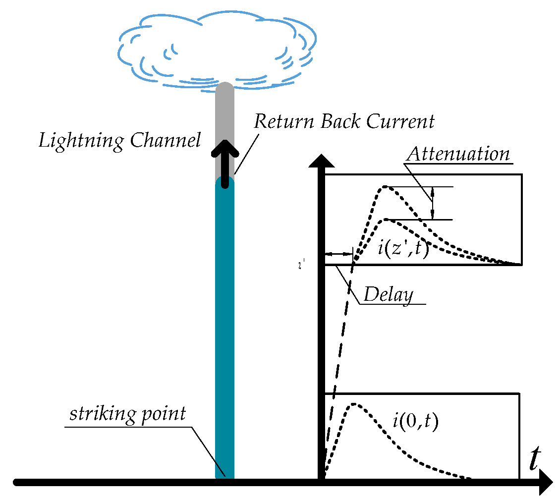There are several engineering models, such as the Bruce–Golde model (BG), transmission line model (TL), traveling current source model (TCS), modified transmission line exponential decay model (MTLE), and modified transmission line linear model (MTLL) [23]. In this paper, the MTLE model is adopted, which can be illustrated as Figure 1 and described by:

$$\{\begin{array}{ll}i(z^{\prime },t)=i(0,t-\frac{z^{\prime }}{v})\exp (-\frac{z^{\prime }}{\alpha }),& t\ge \frac{z^{\prime }}{v}\\ i(z^{\prime },t)=0,& t<\frac{z^{\prime }}{v}\end{array}$$

(1)

where: v—the return stroke velocity along the lightning channel, α—the decaying constant, $i(0,t-z^{\prime }/v)$—the delay of the channel base current, and $\exp (-z^{\prime }/\alpha )$—the attenuation of the channel base current.

As for the channel base current, several functions are available, such as Rubinstein and Uman function, Bruce and Golde function, and Heidler function [24]. In this paper, the channel base current is represented as a sum of two Heidler functions, as given in Equation (2), and the typical parameters are listed in

Table 1. The basic parameters for the channel base current function.

i01	i02	τ11	τ12	τ21	τ22	n1	n2
10.7 × 103 A	6.5 × 103 A	0.25 × 10−6 s	2.5 × 10−6 s	2 × 10−6 s	230 × 10−6 s	2	2

:

$$i(0,t)=\left[\frac{i_{01}}{{\eta }_1}\frac{{\left(t/{\tau }_{11}\right)}^{n_1}}{1+{\left(t/{\tau }_{11}\right)}^{n_1}}\exp \left(-\frac{t}{{\tau }_{12}}\right)+\frac{i_{02}}{{\eta }_2}\frac{{\left(t/{\tau }_{21}\right)}^{n_2}}{1+{\left(t/{\tau }_{21}\right)}^{n_2}}\exp \left(-\frac{t}{{\tau }_{22}}\right)\right],$$

(2)

where:

${\eta }_1=\exp \left(-\frac{{\tau }_{11}}{{\tau }_{12}}{\left(n_1\frac{{\tau }_{12}}{{\tau }_{11}}\right)}^{\frac{1}{n_1}}\right)$ and ${\eta }_2=\exp \left(-\frac{{\tau }_{21}}{{\tau }_{22}}{\left(n_1\frac{{\tau }_{22}}{{\tau }_{21}}\right)}^{\frac{1}{n_2}}\right)$.

2.2. Fundamental Formulation of Lightning Electromagnetic Field over Perfectly Conducting Ground

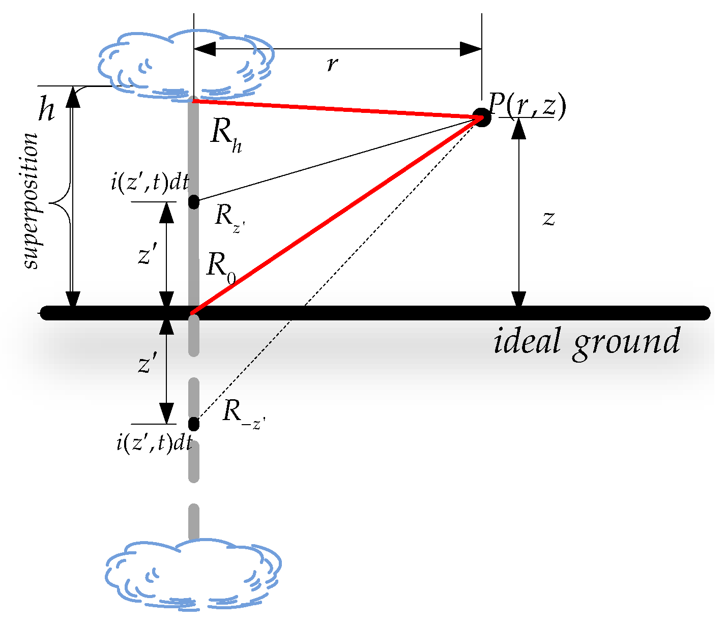
The widely used model of the lightning electromagnetic field over a perfect conducting ground can be illustrated in Figure 2 [25]. The lightning channel can be regarded as a combination of an above-ground lightning channel and its mirror in the free space. Regarding the source as a vertical electric dipole of current $i(z^{\prime },t)d{z}^{\prime }$ located at z′, the formulas of the electromagnetic field at an observation point generated by the lightning channel can be obtained and shown as:

$$\{\begin{array}{l}{E}_{ideal}=\frac{1}{4\pi {\epsilon }_0}\left\{{\displaystyle {\int }_0^h\left[\begin{array}{l}\frac{3r(z-z^{\prime })}{R_{z^{\prime }}^5}{\displaystyle {\int }_0^{t}i(z^{\prime },\tau -R_{z^{\prime }}/c)d\tau }\\ +\frac{3r(z-z^{\prime })}{c{R}_{z^{\prime }}^4}i(z^{\prime },t-R_{z^{\prime }}/c)\\ +\frac{r(z-z^{\prime })}{c^2{R}_{z^{\prime }}^3}\frac{\partial i(z^{\prime },t-R_{z^{\prime }}/c)}{\partial t}\end{array}\right]}d{z}^{\prime }+{\displaystyle {\int }_0^h\left[\begin{array}{l}\frac{3r(z+z^{\prime })}{R_{-z^{\prime }}^5}{\displaystyle {\int }_0^{t}i(z^{\prime },\tau -R_{-z^{\prime }}/c)d\tau }\\ +\frac{3r(z+z^{\prime })}{c{R}_{-z^{\prime }}^4}i(z^{\prime },t-R_{-z^{\prime }}/c)\\ +\frac{r(z+z{}^{\prime })}{c^2{R}_{-z^{\prime }}^3}\frac{\partial i(z^{\prime },t-R_{-z^{\prime }}/c)}{\partial t}\end{array}\right]}d{z}^{\prime }\right\}\\ H_{ideal}=\frac{1}{4\pi }\left\{\begin{array}{l}{\displaystyle {\int }_0^h\left[\frac{r}{R_{z^{\prime }}^3}i(z^{\prime },t-R_{z^{\prime }}/c)+\frac{r}{c{R}_{z^{\prime }}^2}\frac{\partial i(z^{\prime },t-R_{z^{\prime }}/c)}{\partial t}\right]}d{z}^{\prime }\\ +{\displaystyle {\int }_0^h\left[\frac{r}{R_{-z^{\prime }}^3}i(z^{\prime },t-R_{-z^{\prime }}/c)+\frac{r}{c{R}_{-z^{\prime }}^2}\frac{\partial i(z^{\prime },t-R_{-z^{\prime }}/c)}{\partial t}\right]}d{z}^{\prime }\end{array}\right\}\end{array},$$

(3)

where: E_ideal(φ, r, z, t)—ideal horizontal electric field at observation point P(r, z), H_ideal(φ, r, z, t)—ideal tangential magnetic field at observation point P(r, z), h—the height of the lightning channel, ε₀—vacuum permittivity, r—horizontal distance from the lightning channel to point P(r, z), R_z′ and R_−z′—distance from the dipole to point P(r, z), z and z′—the z-coordinate of point P(r, z) and the dipole, respectively, and c—speed of light in vacuum.

The calculation of Equation (3) is commonly based on a numerical integration due to the lack of the analytical formulae of Equation (3), which is called the conventional method in this paper. As can be seen, the integrands in Equation (3) are functions of two variables (t and z′), and the propagation of the current along the channel must be considered when implementing the numerical integration. Therefore, it is somewhat complicated and not easily programmed. Experience indicates that a sufficiently small computational step dz′ is essential to get an accurate result, but this leads to a large number of calculations, resulting in a lengthy calculation time.

Therefore, we doubt whether or not some of the integral can be implemented in an analytical way; if so, the efficiency can be improved, especially for the evaluation of the lighting-induced voltages of a distributed network, in which lightning electromagnetic fields with a great amount of observation points are required to be calculated. In the following sections, an efficient method is achieved, which can calculate most of the integrals in Equation (3) analytically.

2.3. Proposed Method for Calculating the Lightning Electromagnetic Field over Perfectly Conducting Ground

In order to simplify Equation (3), firstly, we transform the system from time varying to time invariant. The process of the channel base current propagating along the lightning channel is time varying, but if regarded it as a current model with i(z′, t) = i_base(t-z′/v) distribution at all points along the channel direction, the system can be transformed into a time-invariant system. Then, we can transform the time-invariant system into the frequency domain based on the Fourier transform. Finally, the analytical formulae for most of the integral in Equation (3) can be obtained by means of some derivations.

Substituting Equations (1) and (2) into (3) and representing the equations in the frequency domain allows the formulas to be rearranged as:

$$E_{ideal}=\frac{1}{4\pi {\epsilon }_0}\left\{\underset{E_{above}}{\underbrace{{\displaystyle {\int }_0^h\left[\begin{array}{l}\frac{3r(z-z^{\prime })}{R_{z^{\prime }}^5}\frac{I(0,j\omega )}{j\omega }{e}^{-z^{\prime }\left(\frac{j\omega }{v}+\frac{1}{\alpha }\right)}{e}^{-jk{R}_{z^{\prime }}}\\ +\frac{3r(z-z{}^{\prime })}{c{R}_{z^{\prime }}^4}I(0,j\omega )e^{-z^{\prime }\left(\frac{j\omega }{v}+\frac{1}{\alpha }\right)}{e}^{-jk{R}_{z^{\prime }}}\\ +j\omega \frac{r(z-z^{\prime })}{c^2{R}_{z^{\prime }}^3}I(0,j\omega )e^{-z^{\prime }\left(\frac{j\omega }{v}+\frac{1}{\alpha }\right)}{e}^{-jk{R}_{z^{\prime }}}\end{array}\right]}d{z}^{\prime }}}+\underset{E_{under}}{\underbrace{{\displaystyle {\int }_0^h\left[\begin{array}{l}\frac{3r(z+z^{\prime })}{R_{-z^{\prime }}^5}\frac{I(0,j\omega )}{j\omega }{e}^{-z^{\prime }\left(\frac{j\omega }{v}+\frac{1}{\alpha }\right)}{e}^{-jk{R}_{-z^{\prime }}}\\ +\frac{3r(z+z^{\prime })}{c{R}_{-z^{\prime }}^4}I(0,j\omega )e^{-z^{\prime }\left(\frac{j\omega }{v}+\frac{1}{\alpha }\right)}{e}^{-jk{R}_{-z^{\prime }}}\\ +j\omega \frac{r(z+z^{\prime })}{c^2{R}_{-z^{\prime }}^3}I(0,j\omega )e^{-z^{\prime }\left(\frac{j\omega }{v}+\frac{1}{\alpha }\right)}{e}^{-jk{R}_{-z^{\prime }}}\end{array}\right]}d{z}^{\prime }}}\right\}$$

(4)

As can be seen in Equation (4), E_above and E_under have the same form, so only the derivation for E_above is provided. The above-ground lightning channel-generated horizontal electric field can be divided into three parts, i.e., E_A, E_B, and E_C, as shown in Equation (5):

$$E_{above}=\frac{I\left(0,j\omega \right)r}{4\pi {\epsilon }_0}\left\{\begin{array}{l}\underset{E_A}{\underbrace{\frac{3}{j\omega }{\displaystyle {\int }_0^h\frac{\left(z-z^{\prime }\right)}{R_{z^{\prime }}^5}\cdot e^{-z^{\prime }\left(\frac{j\omega }{v}+\frac{1}{\alpha }\right)}{e}^{-jk{R}_{z^{\prime }}}d{z}^{\prime }}}}+\underset{E_B}{\underbrace{\frac{3}{c}{\displaystyle {\int }_0^h\frac{\left(z-z^{\prime }\right)}{R_{z^{\prime }}^4}\cdot e^{-z^{\prime }\left(\frac{j\omega }{v}+\frac{1}{\alpha }\right)}{e}^{-jk{R}_{z^{\prime }}}d{z}^{\prime }}}}\\ +\underset{E_C}{\underbrace{j\omega \frac{1}{c^2}{\displaystyle {\int }_0^h\frac{\left(z-z^{\prime }\right)}{R_{z^{\prime }}^3}\cdot e^{-z^{\prime }\left(\frac{j\omega }{v}+\frac{1}{\alpha }\right)}{e}^{-jk{R}_{z^{\prime }}}d{z}^{\prime }}}}\end{array}\right\},\left\{k=\frac{\omega }{c}\right\}$$

(5)

By means of ${\displaystyle \int \frac{\left(z-z^{\prime }\right)}{R_{z^{\prime }}^5}}d{z}^{\prime }=\frac{1}{3R_{z^{\prime }}^3}$ and ${\displaystyle \int u^{\prime }vdz=uv-{\displaystyle \int u{v}^{\prime }dz}}$, E_A can be rewritten as:

$$E_A=\left\{\underset{E_{A1}}{\underbrace{\frac{1}{j\omega }\cdot {\frac{1}{R_{z^{\prime }}^3}{e}^{-z^{\prime }\left(\frac{j\omega }{v}+\frac{1}{\alpha }\right)}{e}^{-jk{R}_{z^{\prime }}}|}_0^h}}+\underset{E_{A2}}{\underbrace{\frac{1}{j\omega }\cdot \left(\frac{j\omega }{v}+\frac{1}{\alpha }\right){\displaystyle {\int }_0^h\frac{1}{R_{z^{\prime }}^3}{e}^{-z^{\prime }\left(\frac{j\omega }{v}+\frac{1}{\alpha }\right)}{e}^{-jk{R}_{z^{\prime }}}d{z}^{\prime }}}}+\underset{E_{A3}}{\underbrace{(-\frac{1}{c}{\displaystyle {\int }_0^h\frac{\left(z-z^{\prime }\right)}{R_{z^{\prime }}^4}{e}^{-z^{\prime }\left(\frac{j\omega }{v}+\frac{1}{\alpha }\right)}{e}^{-jk{R}_{z^{\prime }}}d{z}^{\prime }})}}\right\}$$

(6)

in which E_A2 can be described as Equation (7) based on ${\displaystyle \int \frac{(z-z^{\prime })}{R_{z^{\prime }}^3}}d{z}^{\prime }=\frac{1}{R_{z^{\prime }}}$ and ${\displaystyle \int u^{\prime }vdz=uv-{\displaystyle \int u{v}^{\prime }dz}}$:

$$E_{A2}=\left\{\begin{array}{l}\underset{E_{A21}}{\underbrace{{\frac{1}{j\omega }\cdot \left(\frac{j\omega }{v}+\frac{1}{\alpha }\right)\frac{1}{R_{z^{\prime }}}\frac{1}{z-z^{\prime }}{e}^{-z^{\prime }\left(\frac{j\omega }{v}+\frac{1}{\alpha }\right)}{e}^{-jk{R}_{z^{\prime }}}|}_0^h}}+\underset{E_{A22}}{\underbrace{\left(-\frac{1}{j\omega }\cdot \left(\frac{j\omega }{v}+\frac{1}{\alpha }\right){\displaystyle {\int }_0^h\frac{1}{R_{z^{\prime }}}\frac{1}{{\left(z-z^{\prime }\right)}^2}{e}^{-z^{\prime }\left(\frac{j\omega }{v}+\frac{1}{\alpha }\right)}{e}^{-jk{R}_{z^{\prime }}}d{z}^{\prime }}\right)}}\\ +\underset{E_{A23}}{\underbrace{\frac{1}{j\omega }\cdot \left(\frac{j\omega }{v}+\frac{1}{\alpha }\right)\left(\frac{j\omega }{v}+\frac{1}{\alpha }\right){\displaystyle {\int }_0^h\frac{1}{R_{z^{\prime }}}\frac{1}{z-z^{\prime }}{e}^{-z^{\prime }\left(\frac{j\omega }{v}+\frac{1}{\alpha }\right)}{e}^{-jk{R}_{z^{\prime }}}d{z}^{\prime }}}}+\underset{E_{A24}}{\underbrace{\left(-\frac{1}{c}\cdot \left(\frac{j\omega }{v}+\frac{1}{\alpha }\right){\displaystyle {\int }_0^h\frac{1}{R_{z^{\prime }}^2}{e}^{-z^{\prime }\left(\frac{j\omega }{v}+\frac{1}{\alpha }\right)}{e}^{-jk{R}_{z^{\prime }}}d{z}^{\prime }}\right)}}\end{array}\right\}$$

(7)

As for E_A22, according to ${\displaystyle \int \frac{1}{R_{z^{\prime }}{\left(z-z^{\prime }\right)}^2}}d{z}^{\prime }=\frac{R_{z^{\prime }}}{r^2\left(z-z^{\prime }\right)}$ and ${\displaystyle \int u^{\prime }vdz=uv-{\displaystyle \int u{v}^{\prime }dz}}$, it will be:

$$E_{A22}=\left\{\begin{array}{l}\underset{E_{A221}}{\underbrace{{-\frac{1}{j\omega }\cdot \left(\frac{j\omega }{v}+\frac{1}{\alpha }\right)\frac{R_{z^{\prime }}}{r^2\left(z-z^{\prime }\right)}{e}^{-z^{\prime }\left(\frac{j\omega }{v}+\frac{1}{\alpha }\right)}{e}^{-jk{R}_{z^{\prime }}}|}_0^h}}+\underset{E_{A222}}{\underbrace{\frac{1}{j\omega }\cdot \left(\frac{j\omega }{v}+\frac{1}{\alpha }\right)jk\frac{1}{r^2}{\displaystyle {\int }_0^h{e}^{-z^{\prime }\left(\frac{j\omega }{v}+\frac{1}{\alpha }\right)}{e}^{-jk{R}_{z^{\prime }}}d{z}^{\prime }}}}\\ +\underset{E_{A223}}{\underbrace{\left(-\frac{1}{j\omega }\cdot \left(\frac{j\omega }{v}+\frac{1}{\alpha }\right)\left(\frac{j\omega }{v}+\frac{1}{\alpha }\right){\displaystyle {\int }_0^h\frac{R_{z^{\prime }}}{r^2\left(z-z^{\prime }\right)}{e}^{-z^{\prime }\left(\frac{j\omega }{v}+\frac{1}{\alpha }\right)}{e}^{-jk{R}_{z^{\prime }}}d{z}^{\prime }}\right)}}\end{array}\right\}$$

(8)

Combining E_A3 with E_B and using ${\displaystyle \int \frac{(z-z^{\prime })}{R_{z^{\prime }}^4}}dz{}^{\prime }=\frac{1}{2R_{z^{\prime }}^2}$, we can get:

$$E_{A3}+E_B=\left\{\begin{array}{l}\underset{E_{B1}}{\underbrace{\frac{2}{c}{\frac{1}{2R_{z^{\prime }}^2}{e}^{-z^{\prime }\left(\frac{j\omega }{v}+\frac{1}{\alpha }\right)}{e}^{-jk{R}_{z^{\prime }}}|}_0^h}}+\underset{E_{B2}}{\underbrace{\frac{1}{c}\left(\frac{j\omega }{v}+\frac{1}{\alpha }\right){\displaystyle {\int }_0^h\frac{1}{R_{z^{\prime }}^2}{e}^{-z^{\prime }\left(\frac{j\omega }{v}+\frac{1}{\alpha }\right)}{e}^{-jk{R}_{z^{\prime }}}d{z}^{\prime }}}}\\ +\underset{E_{B3}}{\underbrace{(-j\omega \frac{1}{c^2}{\displaystyle {\int }_0^h\frac{\left(z-z^{\prime }\right)}{R_{z^{\prime }}^3}{e}^{-z^{\prime }\left(\frac{j\omega }{v}+\frac{1}{\alpha }\right)}{e}^{-jk{R}_{z^{\prime }}}d{z}^{\prime }})}}\end{array}\right\}.$$

(9)

$E_{A222}$, $E_{A223}$, and $E_{A23}$ can also be combined, and the summation of them can be expressed as Equation (10), taking advantage of ${\displaystyle {\int }_0^h\frac{z-z^{\prime }}{R_{z^{\prime }}}}{e}^{-jk{R}_{z^{\prime }}}d{z}^{\prime }=\frac{e^{-jk{R}_{z^{\prime }}}}{jk}$:

$$E_{A222}+E_{A223}+E_{A23}=\left\{\begin{array}{l}\underset{E_{A231}}{\underbrace{-{\frac{1}{j\omega r^2}\cdot \left(\frac{j\omega }{v}+\frac{1}{\alpha }\right)\left(\frac{j\omega }{v}+\frac{1}{\alpha }\right)\frac{e^{-jk{R}_{z^{\prime }}}}{jk}{e}^{-z^{\prime }\left(\frac{j\omega }{v}+\frac{1}{\alpha }\right)}|}_0^h}}\\ +\underset{E_{A241}}{\underbrace{\frac{1}{j\omega r^2}\left(\frac{j\omega }{v}+\frac{1}{\alpha }\right)\left[jk-\frac{1}{jk}{\left(\frac{j\omega }{v}+\frac{1}{\alpha }\right)}^2\right]{\displaystyle {\int }_0^h{e}^{-z^{\prime }\left(\frac{j\omega }{v}+\frac{1}{\alpha }\right)}{e}^{-jk{R}_{z^{\prime }}}d{z}^{\prime }}}}\end{array}\right\}.$$

(10)

Considering E_B2 + E_A24 = 0 and E_B3 + E_C = 0, Equation (5) can be rewritten as:

$$E_{above}=\frac{I\left(0,j\omega \right)r}{4\pi {\epsilon }_0}\left\{\begin{array}{l}\underset{E_{A1}}{\underbrace{\frac{1}{j\omega }\cdot {\frac{1}{R_{z^{\prime }}^3}{e}^{-z^{\prime }\left(\frac{j\omega }{v}+\frac{1}{\alpha }\right)}{e}^{-jk{R}_{z^{\prime }}}|}_0^h}}+\underset{E_{B1}}{\underbrace{\frac{2}{c}{\frac{1}{2R_{z^{\prime }}^2}{e}^{-z^{\prime }\left(\frac{j\omega }{v}+\frac{1}{\alpha }\right)}{e}^{-jk{R}_{z^{\prime }}}|}_0^h}}\\ +\underset{E_{A21}}{\underbrace{{\frac{1}{j\omega }\cdot \left(\frac{j\omega }{v}+\frac{1}{\alpha }\right)\frac{1}{R_{z^{\prime }}}\frac{1}{z-z^{\prime }}{e}^{-z^{\prime }\left(\frac{j\omega }{v}+\frac{1}{\alpha }\right)}{e}^{-jk{R}_{z^{\prime }}}|}_0^h}}\\ +\underset{E_{A221}}{\underbrace{(-\frac{1}{j\omega }\cdot \left(\frac{j\omega }{v}+\frac{1}{\alpha }\right){\frac{R_{z^{\prime }}}{r^2\left(z-z{}^{\prime }\right)}{e}^{-z^{\prime }\left(\frac{j\omega }{v}+\frac{1}{\alpha }\right)}{e}^{-jk{R}_{z^{\prime }}}|}_0^h)}}\\ +\underset{E_{A231}}{\underbrace{(-{\frac{1}{j\omega r^2}\cdot \left(\frac{j\omega }{v}+\frac{1}{\alpha }\right)\left(\frac{j\omega }{v}+\frac{1}{\alpha }\right)\frac{e^{-jk{R}_{z^{\prime }}}}{jk}{e}^{-z^{\prime }\left(\frac{j\omega }{v}+\frac{1}{\alpha }\right)}|}_0^h)}}\\ +\underset{E_{A241}}{\underbrace{\left[j\omega \frac{1}{v}\left(\frac{1}{c}-\frac{c}{v^2}\right)+\frac{1}{\alpha }\left(\frac{1}{c}-\frac{3c}{v^2}\right)-\frac{1}{j\omega }\frac{3c}{{\alpha }^{2}v}-\frac{1}{{\left(j\omega \right)}^2}\frac{c}{{\alpha }^3}\right]\cdot \frac{1}{r^2}{\displaystyle {\int }_0^h{e}^{-z^{\prime }\left(\frac{j\omega }{v}+\frac{1}{\alpha }\right)}{e}^{-jk{R}_{z^{\prime }}}d{z}^{\prime }}}}\end{array}\right\}$$

(11)

and it can be transformed into the time domain, i.e.:

$$E_{above}=E_{arithmetic}+E_{integral},$$

(12)

where:

$$E_{arithmetic}=\frac{1}{4\pi {\epsilon }_0}\left\{\begin{array}{l}\left(\frac{r}{c}\frac{1}{R_h^2}+\frac{r}{v{R}_h}\frac{1}{z-h}-\frac{R_h}{vr\left(z-h\right)}-\frac{c}{r{v}^2}\right)i\left(0,t-\frac{h}{v}-\frac{R_h}{c}\right)e^{-\frac{h}{\alpha }}\\ -\left(\frac{r}{c}\frac{1}{R_0^2}+\frac{r}{v{R}_0}\frac{1}{z}-\frac{R_0}{vrz}-\frac{c}{r{v}^2}\right)i\left(0,t-\frac{R_0}{c}\right)\\ +\left(\frac{r}{R_h^3}+\frac{1}{\alpha }\frac{r}{R_h}\frac{1}{z-h}-\frac{1}{\alpha }\frac{R_h}{r\left(z-z^{\prime }\right)}-\frac{2c}{\alpha vr}\right)i^{-1}\left(0,t-\frac{h}{v}-\frac{R_h}{c}\right)e^{-\frac{h}{\alpha }}\\ -\left(\frac{r}{R_0^3}+\frac{1}{\alpha }\frac{r}{R_0}\frac{1}{z}-\frac{1}{\alpha }\frac{R_0}{rz}-\frac{2c}{\alpha vr}\right)i^{-1}\left(0,t-\frac{R_0}{c}\right)\\ -\frac{c}{r{\alpha }^2}{i}^{-2}\left(0,t-\frac{h}{v}-\frac{R_h}{c}\right)e^{-\frac{h}{\alpha }}+\frac{c}{r{\alpha }^2}{i}^{-2}\left(0,t-\frac{R_0}{c}\right)\end{array}\right\}$$

(13)

$$E_{integral}=\left\{\begin{array}{l}\frac{1}{v}\left(\frac{1}{c}-\frac{c}{v^2}\right)\cdot \frac{1}{r}\cdot \frac{d}{dt}{i}_{integral}\left(t\right)+\frac{1}{\alpha }\left(\frac{1}{c}-\frac{3c}{v^2}\right)\cdot \frac{1}{r}\cdot i_{integral}\left(t\right)\\ -\frac{3c}{{\alpha }^{2}v}\cdot \frac{1}{r}\cdot i_{integral}^{-1}\left(t\right)-\frac{c}{{\alpha }^3}\cdot \frac{1}{r}\cdot i_{integral}^{-2}\left(t\right)\end{array}\right\},$$

(14)

where: $i\left(0,t\right)$—the channel base current, $i\left(0,t-\frac{h}{v}-\frac{R_h}{c}\right)$ and $i\left(0,t-\frac{R_0}{c}\right)$—the channel base current with delay, $i_{integral}\left(t\right)=\frac{1}{4\pi {\epsilon }_0}{\displaystyle {\int }_0^{h}i(0,t-\frac{z^{\prime }}{v}-\frac{R_{z^{\prime }}}{c})e^{-z^{\prime }(\frac{1}{\alpha })}d{z}^{\prime }}$—the integral component associated with the channel base current, R_h—the distance between the highest point of the lightning channel and point P(r, z), and R₀—the distance between the lightning strike point and point P(r, z).

By means of the similar derivation, the formula for E_under can also be achieved, only by replacing z–z′ and R_z′ by z + z′ and R–_z′, respectively. Finally, the horizontal electric field E_ideal can be obtained by adding them together.

As can be seen from Equations (12)–(14), almost all of the integral can be evaluated in an analytical way, except for E_integral. Moreover, the numerical calculation of E_integral is very simple, because it only contains the integral of the current along the channel and its derivatives. Generally, comparing Equations (12)–(14) with Equation (3), it can be seen that the proposed method equates the integral operation with a simple arithmetic operation and a simple integral. The arithmetic operation involves fewer steps, requires less data, and produces more accurate results. The integral is much simpler than that of the conventional method. Thus, doing this makes the proposed method more efficient and easily programmed.

3. Results

In order to demonstrate the superiority of the proposed method, some simulations were performed in MATLAB on a PC with i7 CPU. To focus on the difference between the two methods, the discretization step along the lightning channel, dz′, was adopted as the variable, while the other parameters are listed in

Table 2. Basic parameters used in the simulation examples.

t	v	r	z	c	α	dt	ε0
30 μs	1.3 × 108 m/s	50/250/500 m	10 m	3 × 108 m/s	1700 m	10 ns	8.854 × 10−12

. The main purpose of this paper was to deal with the calculation problem of the horizontal electric field and it is noted that the horizontal electric field has great attenuation when it is more than 1 km away from the lightning return channel, so the lightning striking distance r is restricted to 0~1 km. According to the geometric formula, the height difference caused by the curvature of the earth is below 8 cm, which is very small compared with the distance of 1 km [26], so the influence of the curvature of the earth is ignored in this paper.

Since both of the methods include numerical integration with respect to dz′, the value of dz′ would inevitably influence the accuracy. Theoretically, the smaller the value of dz′, the more accurate the result. However, there must be a trade-off between the adoption of dz′ and the efficiency.

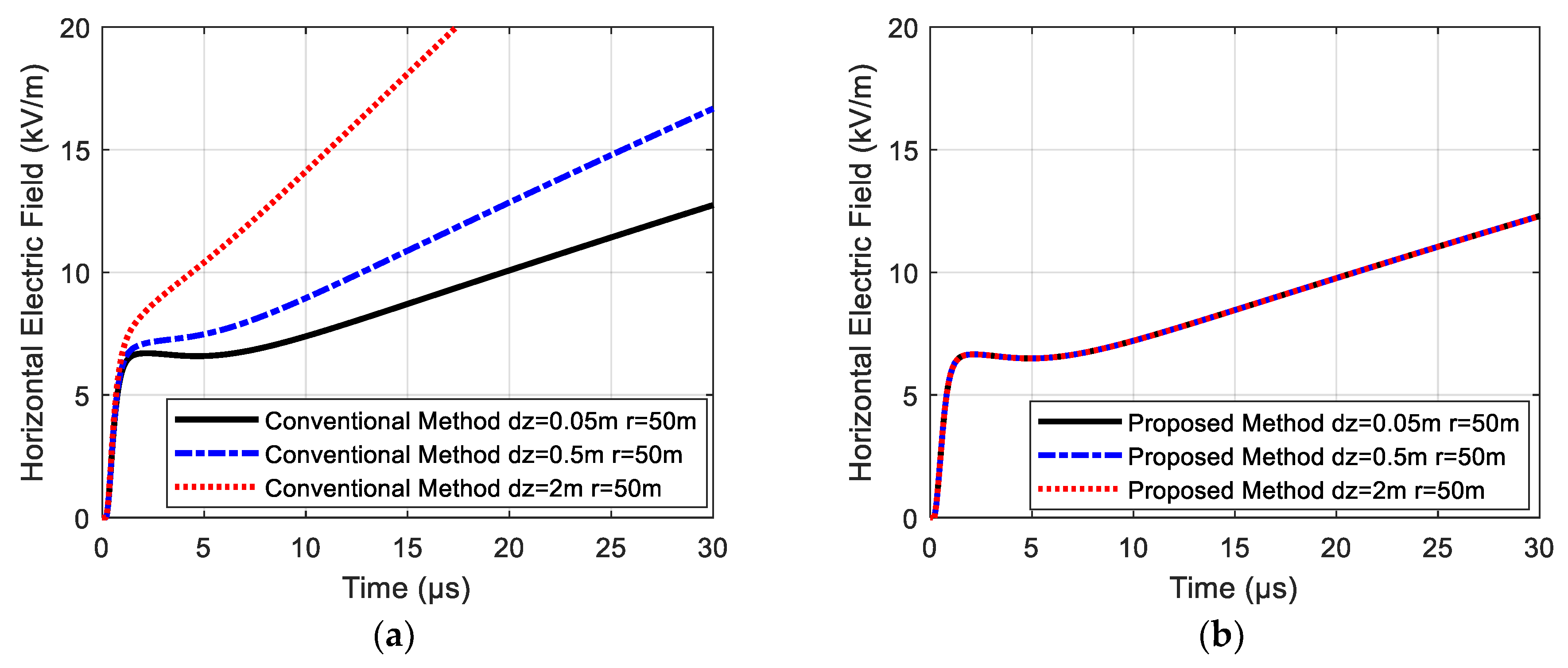
Firstly, the effect of dz′ on the calculation accuracy of the two methods was studied, which is shown in Figure 3. By comparing Figure 3a with b, it can be seen that dz′ has a great influence on the horizontal electric field’s calculation of the conventional method, while it has basically no influence on that of the proposed method. When dz′ ≥ 0.05 m, the horizontal electric field obtained by the conventional method will deviate from the real value. However, no matter what value of dz′ is taken by the proposed method, the final calculation results are consistent. Therefore, the proposed method is more accurate when the dz′ is the same.

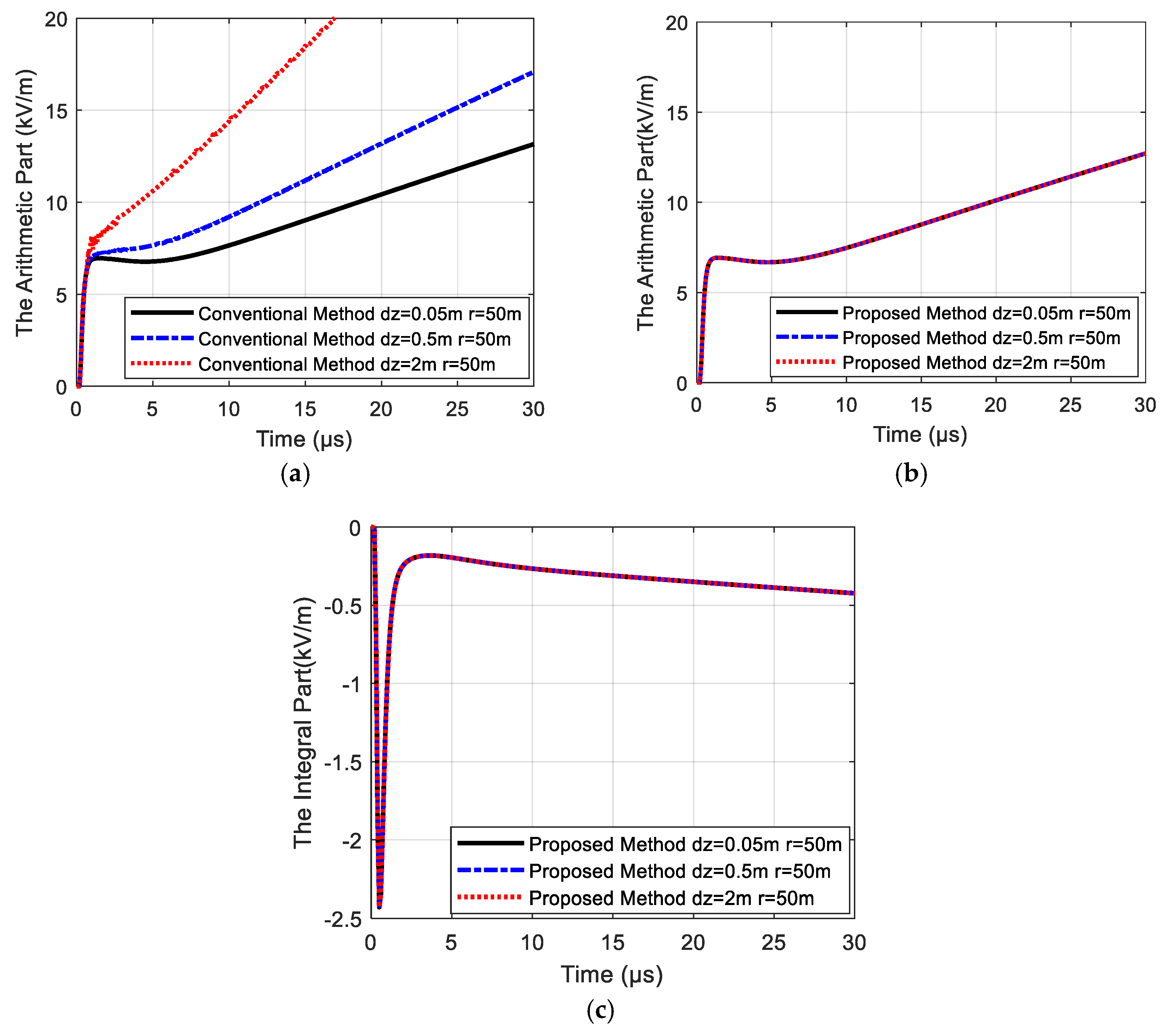
The calculation formulae of the proposed method are composed of two parts: The arithmetic part as shown in Equation (13) and the integral part as shown in Equation (14). In order to better explain the reason why the proposed method is not sensitive to dz′, these two parts were analyzed respectively. For the arithmetic part, it is an error-free analytical result completely independent of dz′ in the proposed method (analytical calculation) while an inexact numerical result sensitive to dz′ in the conventional method (numerical calculation), as shown in Figure 4a,b. This indicates that the proposed method is more accurate in this part than the conventional method. For the integral part, its accuracy would be dependent on dz′. However, as can be seen in Figure 4c, the results are coincident together, although dz′ takes different values. That is to say, an adoption of dz′ = 2 m is enough to achieve the accurate result. This is why the proposed method can guarantee the accuracy with a relatively larger dz′.

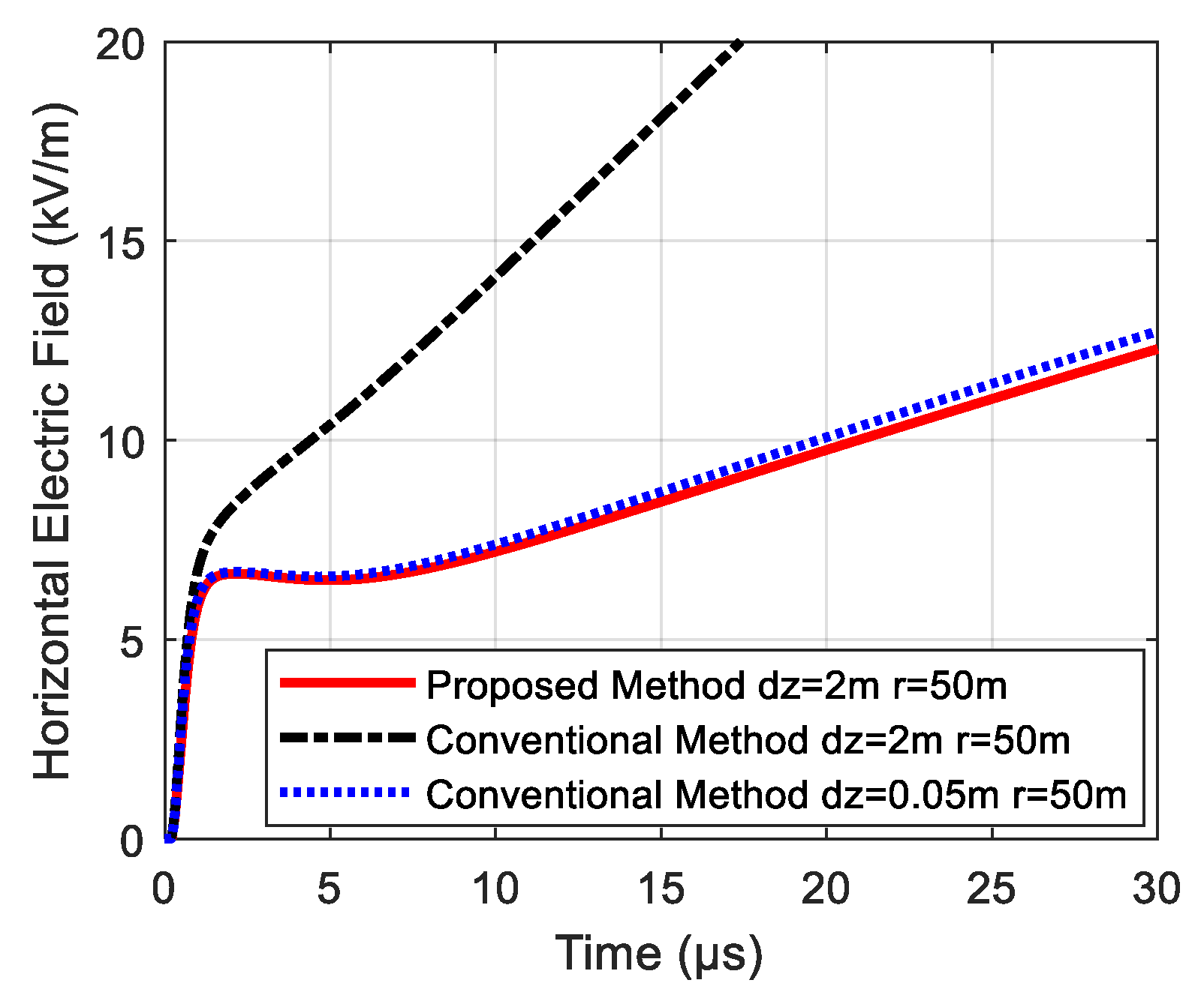
The most fundamental reason why the proposed method can improve the efficiency can be well explained by Figure 5. It can be seen that the horizontal electric field calculated by the proposed method under a condition of dz′ = 2 m is close to that of the conventional method with dz′ = 0.05 m, and the computation time is 0.143 and 5.776 s, respectively, as shown in

Table 3. Comparison of the computation time between two methods.

dz′	Conventional Method	Proposed Method
0.05 m	5.776 s	-
2 m	0.121 s	0.143 s

. That is to say, the acceleration of the proposed method is more efficient than that of the conventional method with the same accuracy.

Considering the calculation of lightning-induced voltages of distributed overhead lines, it is often necessary to calculate a large number of observation points. Taking a one-kilometer three-phase line network as an example, it is generally necessary to calculate at least 300 observation points. According to Table 3, the computation time of the proposed method will be about 1 min. It can be imagined that the more complex the power networks studied, the more efficient the proposed method. Additionally, compared with the conventional method, the proposed method is easier to be programmed because the only formula required to be calculated numerically is very simple.

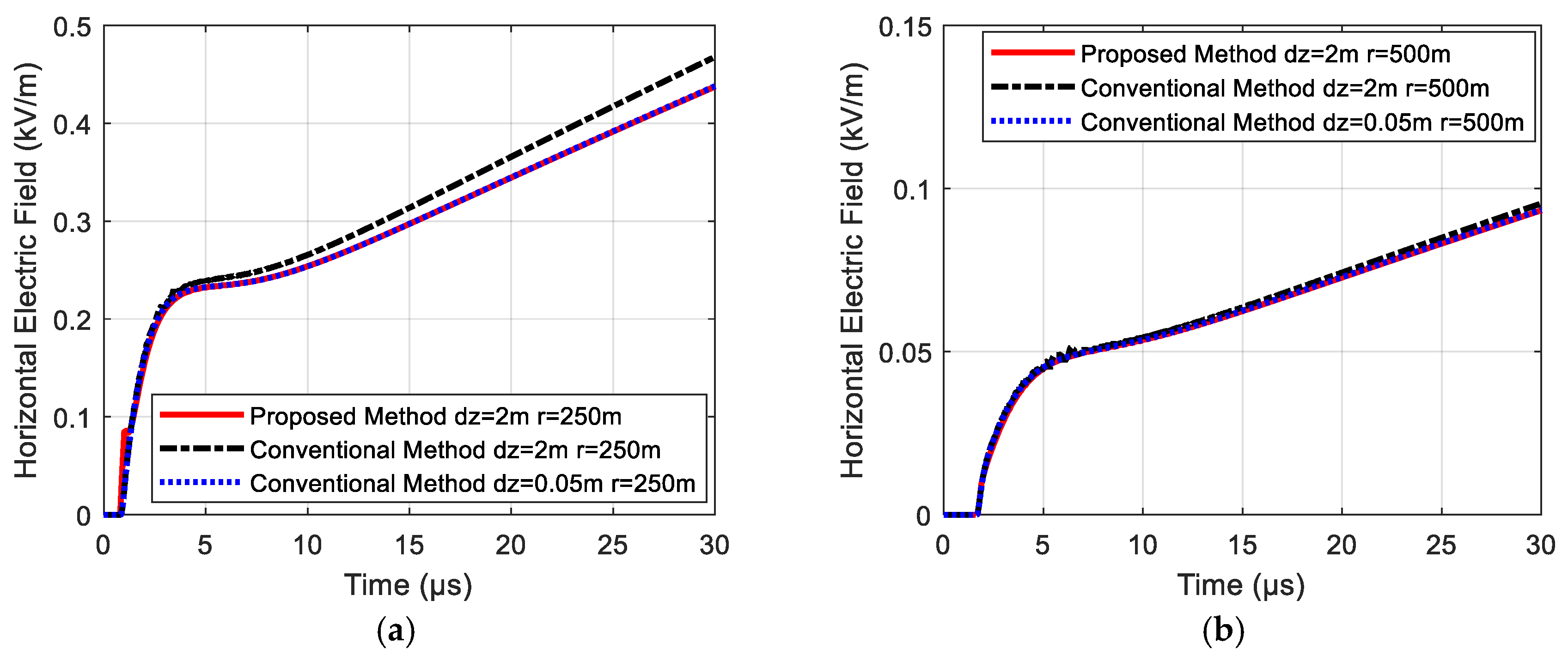
We also considered the cases of r = 250 and 500 m. In these examples, the static E-field component of the horizontal electric field will gradually decrease, but the advantages of the proposed method still remain. The comparison of the two methods is shown in Figure 6 and

Table 4. Comparison of the computation time between the two methods.

dz′	Conventional Method		Proposed Method
-	r = 250 m	r = 500 m	r = 250 m	r = 500 m
0.05 m	4.688 s	4.673 s	-	-
2 m	0.203 s	0.163 s	0.150 s	0.142 s

. It can be seen from Figure 6b that the horizontal electric field calculated by the conventional method with dz′ = 2m is close to the one with dz′ = 0.05 m when r reaches more than 500 m. The efficiency of the two methods is almost the same, as the computation time listed in Table 4. However, as for the relative closer observation points, such as r = 250 m, small dz′ is still required, which can be examined in Figure 6a. In a word, as for the conventional method, small dz′ should be adopted for the observation point near the lighting channel, while large dz′ can be used for the observation point far away. However, in the proposed method, small dz′ can be adopted no matter the distance from the observation point and the lightning striking point, which indicates that the proposed method is more general. In other words, the proposed method can adopt uniform dz′ without considering the different lightning striking distances. Therefore, its implementation is more convenient. Additionally, as the statement above, the proposed method is easier to be programmed because the formulation of the item for numerical integration is simpler, which is superior to the proposed method.

It should also be pointed out that the horizontal component of the lightning electric field attenuates greatly with the distance, as shown in Figure 4, Figure 5 and Figure 6. Considering the lightning striking distances of more than 500 m, the overvoltage induced by the lightning electromagnetic field on the power line is generally small, which poses little threat to the insulation. Therefore, the example of the horizontal component of the lightning electric field at a longer distance is not discussed in this paper.

As for the calculation of the magnetic field near the lightning channel, its formula can be derived in the same manner as the horizontal electric field. It is not described in this paper for the sake of brevity.

4. Discussion and Conclusions

For the calculation of lightning electromagnetic fields over a perfectly conducting ground, the common method is to evaluate the integral by means of numerical integration. In the proposed method, the formula for calculating the lightning electromagnetic field is divided into two parts: One that can be solved analytically, and the other that can be solved numerically only by integral operations.

For the conventional method, the results are sensitive to dz′ at a close distance (tens of meters), which must be small enough to get an accurate numerical solution. However, when dz′ is too small, the amount of data required in the program is huge and the calculation steps are tedious, resulting in a lengthy time and slow calculation speed. As for the proposed method, dz′ can be adopted as a relatively large value, so the computational efficiency can be improved inevitably. Two calculation methods were simulated in MATLAB, of which the simulation results showed that under the same accuracy, the calculation time of the proposed method is about 1/40 of that of the original method. As for large lightning striking distances (hundreds of meters), the conventional method’s results are not sensitive to dz′ anymore, and relative larger dz′ can be adopted to get an accurate numerical solution. In other words, for the conventional method, small dz′ should be adopted for the observation point near the lighting channel while large dz′ can be used for the observation point far away. However, the proposed method has better generality because it can calculate the horizontal electric fields at different lightning striking distances with a uniform dz′, which makes its implementation more convenient and easily programmed. Additionally, as can be seen, the only item required to be calculated numerically is very simple and other items can be implemented in an analytical way, so the proposed method is very easy to be programmed, compared with the original method.