Analysis of Optimal Flight Parameters of Unmanned Aerial Vehicles (UAVs) for Detecting Potholes in Pavements

Abstract

Pavement maintenance seeks to provide optimal service conditions. Before maintenance, it is necessary to know the condition of the pavement by inspection, a crucial step in deciding on the repair to be carried out. In this sense, unmanned aerial vehicles (UAVs) seem to be an economic substitute compared to the ground laser scanner for pavement inspection tasks. This research seeks to develop a method to measure potholes using 3D models generated with photographs acquired by a UAV and process them using a software based on the Structure from Motion-MultiView Stereo (SfM–MVS) technique. The contribution of this document is the proposal of recommendations for the acquisition of photographs for the realization of the models. To develop these recommendations, an experiment was carried out to evaluate the accuracy in the reconstruction of 3D models using images obtained from the variation and combination of flight planning parameters and data capture. Then, to validate these recommendations, a bumpy section of pavement was modeled using the SfM–MVS method. The results show that for heights of 10 and 15 m the use of this methodology is applicable for the measurement of the width and depth of potholes.

1. Introduction

The maintenance of roads is a procedure that seeks to deliver optimal service conditions for the routes, generating the least possible impact on the regularity of vehicle flow during operation [1]. Prior to maintenance, it is necessary to know the physical and functional condition of the road, which requires extensive inspection work, focused on knowing its level of damage. It aims to provide measures to assess the magnitude of various types of pavement deterioration, delivering the overall condition of the pavement and providing an estimate of the amount of resources needed to preserve the infrastructure [2]. Inspection is crucial to decide the type and extent of repair a road should receive, and thus provide the desired level of service to maintain acceptable conditions for vehicle traffic [3].

Traditional manual road inspection is time consuming, labor intensive and subjective [2]. Some automated methods, which use equipment with cameras or laser technology, have also been implemented in pavement inspection, greatly improving the efficiency and objectivity of inspection [4]. However, multiple trips may be required to cover the entire width of the road with the inspection vehicle. In addition, the on-the-spot inspection process affects traffic flow, which is particularly unfavorable on high-traffic roads. Unmanned aerial vehicles (UAVs) have the advantage of high flexibility, relatively low cost compared to inspection vehicles, easy maneuverability and less work on the ground [5]; therefore, they are promising in the task of assessing the condition of the pavement.

On the other hand, recent advances in both high-resolution optical cameras and image processing techniques have allowed three-dimensional (3D) models of UAV images to be derived with sufficient accuracy and high efficiency, making image-based 3D models a possible substitute or more economical supplement to 3D laser scanning. Currently, 3D models can easily be generated from images obtained with UAVs. There are several existing 3D modeling programs on the market which can do this automatically.

This article focuses on the measurement of potholes in asphalt pavements, namely depth, width and volume, using a 3D model derived from UAV images. This document aimed to use photographs obtained with a UAV platform and subsequently process them with the Structure from Motion-MultiView Stereo (SfM–MVS) method, in order to perform a better inspection with the primary goal of detecting potholes in pavements. The main contribution of this document is the proposal of recommendations for measuring the geometric characteristics of potholes based on 3D models.

In order to develop these recommendations, an experiment was conducted to evaluate the accuracy in the reconstruction of 3D models using images obtained from the variation and combination of different parameters of flight planning and data capture (digital photographs). Specifically, variations in the combinations of camera angles (vertical–oblique), image overlaps and flight height, relative to a study surface that simulates deteriorating pavement with bumps of different sizes, with the specific purpose of extrapolating the results to actual pavement. The accuracy was evaluated from the comparison of the actual values against the measurement made in each of the 3D models reconstructed from the data obtained by each flight, according to each of the defined mission plans. Bumpy pavement is modeled using the SfM–MVS technique with photographs acquired using the recommendations and via a UAV platform. A comparison of the geometric characteristics (depth, width and volume) of pavement potholes—measured in a 3D model versus those collected in field inspection—demonstrates that the use of the recommendations when extrapolated to real cases is applicable in the practice of pavement inspection.

2. Materials and Methods

For the development of this research, the methodology in Design Science Method (DSRM) was used as the base [6,7,8,9]. Tool components and activities were added to show the research done in more detail. In general, the research methodology is organized into five stages: (1) Identification of observed problems and motivations; (2) Goal definition of the potential solution; (3) Design and development; (4) Demonstration; and (5) Evaluation. Figure 1 specifies the activities and research tools that describe the scenario for each stage.

In the first stage, a literature review was carried out to identify emerging technological tools and problems used in pavement inspection and to define the advantages, disadvantages and potential of using a UAV platform in conjunction with the SfM–MVS method. The literature review was carried out through the web databases of Web of Science and Scopus. In the second stage, the research objective was defined. In the third stage, a solution was designed for the application of a project with UAV-SfM–MVS. This project seeks to materialize the previous scenario. This solution is expected to deliver a clear workflow for the acquisition and processing of images obtained through a UAV platform using the SfM–MVS technique. In the fourth stage, a study surface was generated, which represents different sizes of potholes on a pavement. This study surface sought to demonstrate the expected use of the solution created through its 3D modeling by multiple combinations of variables. Finally, the conclusions obtained were translated into practical recommendations for the solution. In the fifth stage, the solution and recommendations obtained in the previous stage were evaluated through a comparison with a real case study. Finally, at this same stage, the fulfilment of the main research objective is questioned, in addition to future work related to the solution.

2.1. Background

The maintenance of roads, asphalt or concrete, is a procedure that seeks to deliver optimal service conditions to roads, generating the least possible impact on the regularity of the vehicle flow while doing so [1]. Prior to the maintenance work, it is necessary to know the physical and functional condition of the road, requiring extensive inspection work, focused on knowing its level of damage [5]. It provides measures to assess the magnitude of various types of pavement deterioration, delivering the overall condition of the pavement and providing an estimate of the amount of resources needed to preserve the infrastructure [2]. Inspection is the crucial element in deciding the type and extent of the repair that a road should receive, in order to provide the desired level of service and to maintain acceptable conditions for vehicle traffic [3].

The condition of pavement can be studied from two perspectives: structural failures or functional failures. The first refers to the collapse or breakage of one or more layers of pavement, preventing it from withstanding loads on the surface. The second type of failure causes a deterioration in the surface of the pavement, namely unevenness, cracks and formation of potholes, decreasing the service and standard levels of the pavement, causing inconvenience to passengers and negative impact on vehicles [10,11]. A deterioration is an irregularity on the surface of the road which affects the comfort and safety of the vehicle driver. As seen in [12], there are five categories of impairment: (1) cracks by fatigue, block cracks, longitudinal cracks, cross cracks and reflected cracks; (2) deteriorated patches and potholes (it should measure at least 15 cm in diameter); (3) pavement surface deformations, which include ripples and hollowing; (4) surface defects consisting of all deformations that affect the top layer of the pavement; and (5) berm descent, emergence of fines and water, and separation between the berm and pavement.

2.1.1. Traditional Methods for Inspecting Pavement Deterioration

Manual methods were for many years the traditional approach to carrying out pavement inspection [13]. The manual method is to propose a sectioning of the road in different inspection units in its length and width, achieving a detailed review. The revised units are usually at least 15 m long and can be up to four lanes wide, being inspected from a moving or walking vehicle, where the inspector visually identifies defects, and the affected area is estimated as a fraction of the road surface; this data is transferred to paper forms that are taken to the site [14]. This manual approach is costly, laborious, dangerous, subjective and tends to lead to inconsistencies in measurements [15,16].

With the motivation of an automated approach and to minimize these inconsistencies and disadvantages, technologies and procedures have emerged for data collection or processing [2]. The first clear benefit of an automated approach is the reduction of errors associated with transferring data from paper forms used in manual methods. The first way to collect data was through analog images. This consists of photographing the surface of the pavement, usually with 35-mm film. Generally, a downward-facing camera and, if possible, one or more forward-looking cameras or in other configurations, is installed in an inspection vehicle for data capture. Another technology for collecting data is through digital images which can be processed directly by computers. Like analog technology, these cameras are installed in an inspection vehicle, obtaining high-resolution images, higher than normal analog cameras [17]. Methods that use area scanning cameras refer to a photo that represents an area of pavement defined by thousands of pixels. One last technology is that of 3D lasers. This technology uses a laser radar, which uses an exploration laser and reflector to measure reflection times across the pavement surface, thus establishing a three-dimensional pavement surface [18].

On the other hand, data processing technologies can be divided into two groups. In the first group, the process is mainly manual and involves a trained evaluator sitting in a workstation where the images of the pavement are systematically reviewed, and the different deteriorations are identified and classified. In addition, the process is very demanding, as testers must be able to coordinate the simultaneous use of several monitors while tracking observed deteriorations and entering those observations into a rating software [19]. In the second group, fully automated in the context of crack analysis, involves the use of digital recognition software capable of recognizing and quantifying grayscale variations that are related to cracks or cracks on a pavement surface [20]. Various authors [21,22,23,24,25,26] have published methods based on computational algorithms for automatic detection of deterioration; however, these have mainly focused on crack detection, with the exception of [27] which detects two types of deterioration.

2.1.2. New Technologies for Inspecting Pavement Deterioration

Among the technologies available for detection of deterioration in pavement, the laser scanner is one of the most recent [28]. It is based on two principles: flight time and phase change. Flight time sensors estimate the distance between the target and the instrument center by measuring the elapsed time between the emitted and reflected signal, while phase shift sensors are based on the measurement of angular displacement between the emitted and reflected signal. The output obtained from this technology is a dense point cloud. The point cloud, in conjunction with algorithms, can be used to automatically detect road potholes [29]. In addition, the point cloud can be used for general road asset management due to the large amount of information it contains [30,31]. Lasers have been proven to provide high accuracy but it is an expensive resource [32]. In response to the above, coupled with recent advances in both high-resolution digital cameras and image processing techniques, it is now possible to derive three-dimensional models from images obtained, for example, from a UAV, with sufficient accuracy and high efficiency [33,34]. Therefore, image-based three-dimensional models can be an economical substitute for three-dimensional laser scanners [35].

A UAV is an aerial vehicle that can fly without a human pilot [36]. UAVs have become extremely popular, especially in civil applications, due to their low cost and practicality [36,37,38,39]. A growing area of interest for UAV applications is the periodic inspection and evaluation of infrastructures, which is currently an expensive and time-consuming task [40]. Research has already been carried out that evaluates the UAV as a technology for data capture in pavement inspection applications, with good results due to many advantages it has [10,16]. The operating cost for road network inspection is potentially lower than that of using monitoring vehicles. UAVs can approach scenes that would otherwise be difficult to access or even unattainable under safe circumstances [41]. However, at a certain flight height, the spatial resolution of these images limits the ability to detect certain pavement deteriorations, such as individual cracks, because their widths may be less than 1 cm. In addition, especially due to legal limits and battery life, this technology is not usually an alternative as the length of the road to map increases [35].

For 3D reconstruction from image processing, one of the techniques currently used is Structure from Motion (SfM). For reconstruction, SfM relies on images taken from many points of view [42]. Commonly, processor reconstruction is referred to as SfM. However, it is only a step in the flow of image processing (process for 3D reconstruction). Precisely, this step begins after a key point filtration, where the Scale Invariant Feature Transform (SIFT) algorithm and its variations are the most common approaches [43]. Typically, the SfM process ends with two outputs, a scattered point cloud, and camera parameters and image parameters. A scattered point cloud is an intermediate step in the production of much denser point clouds. These dense point clouds are produced by a process called Multi-View Stereo (MVS) from known intrinsic and extrinsic camera parameters. Comparatively, in a dense point cloud versus a scatter, the points are at least two orders of magnitude denser than the sparse point cloud [44].

Data processing begins with feature detection, by identifying common points in several different photos. Because of the fact that there are geometric distortions, it is necessary to find feature points, which are invariant to changes in scale and orientation in order to make matches across a wider region [45]. A filtration process is then applied to the characteristic or key points to ensure that only correct matches remain [43]. After SfM is executed, what is obtained from this step is a 3D reconstruction of the scene, camera positions and orientations, and the camera’s intrinsic parameters. This reconstruction lacks absolute distance between camera poses and between points because scale cannot be recovered from a monocular camera alone [46]. Scaling and georeferencing in the monocular camera case require a minimum of three control points; that is, points raised by topography that serve as the basis for the georeferencing. Another alternative is by using known camera positions obtained from GPS measurements and an inertial measurement unit (IMU) [47]. Finally, the MVS process is responsible for rebuilding a dense point cloud (increasing the number of point clouds obtained from the previous process) [44].

2.2. Image Acquisition and Processing

Structure from Motion (SfM) is a technique for generating a three-dimensional reconstruction from 2D images. Unlike traditional photogrammetry, which Bonneval says [48] is “the technique that aims to accurately study and define the shape, dimensions and position in the space of any object using essentially measurements made on one or more photographs,” SfM uses computer vision algorithms to identify matching characteristics in a set of overlapping digital images, calculating the location and orientation of the camera. Based on these calculations, overlapping images can be used to reconstruct a structure using a 3D point cloud of the object, surface, or photo scene. It is possible to refine and densify the 3D structure generated by SfM using Multi-View Stereo (MVS), thus completing the SfM–MVS workflow, requiring photographs acquired by means of an optical sensor. For the reconstruction process to be successful, a large number of well-exposed photographs of the object, scene or surface of interest must be obtained at the stage of image acquisition, i.e., with a balance between shutter opening, shutter speed and ISO to correctly capture light. In addition, with sufficient resolution and overlap so that the computer vision algorithm can work effectively. The following are the steps of the method used for image acquisition and processing processes, which are schematically detailed in Figure 2.

The technique of acquiring photographs from a UAV comes from a block of photographs formed from parallel flight lines, flown in a snake pattern at a stable altitude, with a constant overlap and a vertical camera angle (90°) [49]. However, the integration of oblique photographs can reduce the systematic deformation resulting from inaccurate calculation to determine the internal geometry of the camera in the modern SfM–MVS photogrammetry [50,51]. There is evidence that oblique photographs contribute to the integrity of the point cloud reconstruction [52].

Some recommendations for the acquisition of images are as follows: each point of the area of interest should appear in at least three images acquired at different positions; capture a static scene; use constant light, so that the color of the features does not vary; avoid overexposed or underexposed images; avoid blurry images, slow shutter speed or camera movement; and avoid transparent, reflective or homogeneous surfaces, as these surfaces cause difficulties in further processing [53].

An operational challenge of reconstruction through photographs captured from a UAV is to determine the optimal flight parameters required to achieve a better rebuild quality without excessively increasing flight time or processing. There are key aspects that determine the quality of the reconstruction of the image, mainly the solution of the reconstruction and the location accuracy of the points that rebuild the model. To find an adequate ratio between quality and efficiency, the UAV operator has a set of flight parameters to be adjusted; this includes the height and flight speed, image overlap and camera angle, among other technical sensor parameters such as ISO, shutter speed and shutter opening. The overlaps between images should be high enough to correctly produce 3D models, usually requiring front overlap of more than 75% (adjusted by varying the number of images per second) and the side overlap of more than 60% (critical variable adjusted in UAV flight path planning) [54]. The influence of lateral overlap on reconstruction is not well established, compared or tested despite its influence on flight efficiency [55].

For flight planning, it is important to consider the scale of the photographs, which will limit the detection and consequently the accuracy of the size of the objects in 3D reconstruction. This requires predefining a spatial resolution on the ground or the ground sampling distance called the Ground Sample Distance (GSD) used to define the resolution of the digital image, as it is the representation of the pixel in the terrain [48,56]. The correlation between the flight, sensor and image parameters implies inevitable trade-offs between the different factors. That is, features based on the UAV platform, such as altitude and its resistance (flight time), but also geometry and image quality, and processing time. For example, it is clear that the higher the altitude, the more area is covered on the ground and the more area you can fly on one battery charge. At the same time, higher altitudes lead to fewer images per unit area that need to be processed. Unfortunately, altitude also directly affects achievable GSD and therefore the details that can be detected from images. It follows that lower altitudes lead to more images per unit area, resulting in other compensation related to data processing. The higher the spatial resolution (increase in the accuracy) of the sensor, i.e., the larger the images and the more images are processed per unit area and the higher the processing times [57].

The workflow (2) of Figure 2 is based on the SfM–MVS approach to 3D reconstruction models from a set of images in which intrinsic calibration parameters (or internal parameters, are focal length and lens distortion) and extrinsic (used to describe the transformation between the camera and the world) are unknown.

To apply the SfM–MVS technique, it is key to start with the feature detection process. A feature is a relevant part of an image that can refer to specific structures in the image itself, ranging from simple structures such as points or edges to more complex structures such as objects. These must be detected by robust methods in order to be able to locate the same characteristics in successive images regardless of image rotation, scale or changes in lighting [45]. Once key points (relevant characteristics) have been located in each image, their matches must be determined in the successive images of the captured set [43,58]. SfM aims to simultaneously reconstruct the 3D scene structure, positions and orientations of the camera, along with intrinsic calibration parameters. Initially, camera positions are estimated roughly, as photographs with different orientation are mapped and correlated along with common feature sets, assuming that the camera’s internal geometry is constant throughout the process [59]. The initial positions of the camera are refined iteratively as more and more solutions are available, which generates the initial point cloud [60]. The point cloud reference system is relative because at this point only relative locations of the camera and scene geometry are obtained [59].

If you need to get a georeferenced SfM model, there are two options: provide camera positions or use ground control points (GPPs). GPPs are artificial targets or natural objects within the area to be mapped with a known position, which can then be identified and used to orient the final model in the computerized work environment. Alternatively, georeferencing and scaling can be performed from known camera positions derived from differential GPS (dGPS) measurements and an inertial measurement unit [47,61]. Even the latter tools are complementary to using control points (a visually identifiable point, which is known to be exactly positioned) on land, as direct georeferencing is used to provide approximate camera locations and then uses external GCP to obtain a more accurate solution [47,62].

Before you apply MVS to the point cloud, there is an optional additional step that may be required in projects with large image sets. As the number of images increases, the computational load of such a focus increases rapidly [63]. RAM requirements increase with the number of images used in rebuilding and set a practical limit on the number of images that can match simultaneously. The solution to this is the grouping of images, that is, splitting a large project into chunks. In [63], there is detailed a pre-processing step known as “grouping views” for MVS (CMVS), which is a method by which the image set is broken down into overlapping view groups to allow dense MVS reconstructions to run in separate groups. The point clouds obtained from the SfM stage is used as a reference for the MVS algorithm, so that it densifies this point cloud, and thus provides a complete reconstruction of the scene [44]. With the dense point clouds containing a wide metric formation on the scanned surfaces, as well as that relative to their color and reflectivity of the material, it is possible to obtain different end products for analysis, such as orthomosaic and DSM.

2.3. Experiments

The purpose of the experiment is to evaluate the accuracy in the reconstruction of 3D models using images obtained from the variation and combination of different parameters of flight planning and data capture (digital photographs); specifically, variations in the combinations of camera angles (vertical-oblique), image overlaps and flight height, relative to a study surface that simulates a deteriorating pavement with bumps of different size, with the specific purpose of extrapolating the results to actual pavement. Accuracy was assessed from the comparison of the actual values versus the measurement made in each of the 3D models reconstructed from the data obtained by each flight, according to each of the defined plans.

The study surface corresponds to a rectangular prism of plaster, which has been treated with surface paint for the purpose of simulating the characteristic color of an asphalt pavement, as seen in the Figure 3. Seven concave surfaces of different sizes were made on the study surface, the characteristics of which are exposed in

Table 1. Characteristics of studio surface potholes.

Pothole [#]	Diameter [mm]	Deep [mm]	Volume [cm3]	Severity Level
1	19.0	8.5	1798	Low
2	37.0	21.0	13,274	Low
3	57.0	27.0	48,478	Low
4	79.0	38.0	129,102	Middle
5	100.0	50.0	261,804	Middle
6	151.0	74.0	901,373	High
7	200.0	101.5	2,094,398	High

, each responding to different sizes and severities, according to [12], to assess the capture sensitivity of the sensor or camera. There are three levels of severity to classify potholes: low severity is a pothole with a depth less than 30 mm, mean severity is between a depth of 30 to 50 mm and high severity must be greater than 50 mm.

Data capture from the study surface was performed in a place free of objects that may cause shadow. In addition, these were made on sunny days, starting the capture of images at 12:52 P.M. until 14:52 P.M. (hours with less shadow), without the presence of clouds that could alter the color tones in the images.

The combination of analyzed variables includes the incorporation of oblique photographs into the set of photographs taken perpendicular to the terrain (vertical), overlap between photographs and flight height. The values of the variables and the justification of that value are detailed below:

• Incorporation of oblique photographs into a set of vertical photographs; due to the lack of research on the effect of incorporating vertical photographs with oblique images and their influence on the accuracy of the 3D model in cases of pavement inspection, this research was carried out in order to evaluate the accuracy of the results obtained through this configuration, which combined the cases of 90°, 90°–80°, 90°–70°, 90°–60°, 90°–45°. Vertical photos with any combination have twice as many images compared to 90°, as it only has the corresponding set of photos.
• Overlap: the longitudinal/transverse percentage overlap considered for the development of the research was 75/68, 80/72, 85/77 and 90/81. These overlapping levels covered the vast majority of usual configurations according to state of the art for road inspection cases.
• Heights: The heights considered for analysis are 2, 5, 8, 10, 15, 20, 25, 30 and 40 m. This is because it is intended to achieve precisions of under one centimeter, so 40 m would be the limit in terms of the value of GSD (GSD (40 m) × 1.07 cm/pixel).

In summary, 180 configurations are shown in Figure 4. These describe the combination of the variables that influence the accuracy of the model obtained by UAV SfM–MVS.

Considering that the area of the study surface is smaller than the area that will capture the UAV in a single image, the area to be captured for 3D reconstruction will be given by images containing a fraction or the entire study surface for each of the variable combinations set out above.

For the development of the experiment, the Phantom 4 Pro UAV was used as a digital imaging tool, the flight characteristics of which are shown in the following

Table 2. UAV Phantom 4 Pro flight features.

Resolution [MP]	Focal Distance [mm]	Shutter Speed [s]	Sensor Size [mm]
20 (5472 × 3648)	8.8	$\frac{1}{2000}$ a $\frac{1}{8000}$	12.83 × 7.22

.

3. Results and Discussion

In this section, the results are displayed in four parts: (1) different flight plans to assess the influence of the angle on the variation of the error; (2) different flight plans to assess the influence of overlap and height on the variation of the error; (3) the selection of optimal parameters; and (4) the case study to validate the recommendations and results. The analysis of the results was made by the relative error presented by each pothole according to its actual characteristics.

3.1. Angle Variation

In

Table 3. Height and overlap of each combination, associated with Figure 5, Figure 6 and Figure 7.

Combination [#]	Height [m]	Overlap [%]	Combination [#]	Height [m]	Overlap [%]
C1	2	75	C19	15	85
C2	2	80	C20	15	90
C3	2	85	C21	20	75
C4	2	90	C22	20	80
C5	5	75	C23	20	85
C6	5	80	C24	20	90
C7	5	85	C25	25	75
C8	5	90	C26	25	80
C9	8	75	C27	25	85
C10	8	80	C28	25	90
C11	8	85	C29	30	75
C12	8	90	C30	30	80
C13	10	75	C31	30	85
C14	10	80	C32	30	90
C15	10	85	C33	40	75
C16	10	90	C34	40	80
C17	15	75	C35	40	85
C18	15	80	C36	40	90

, the series are presented (named C1-C36 and associated with Figure 5, Figure 6 and Figure 7) associated with different combinations of height and overlap. Each series includes the five angle combinations.

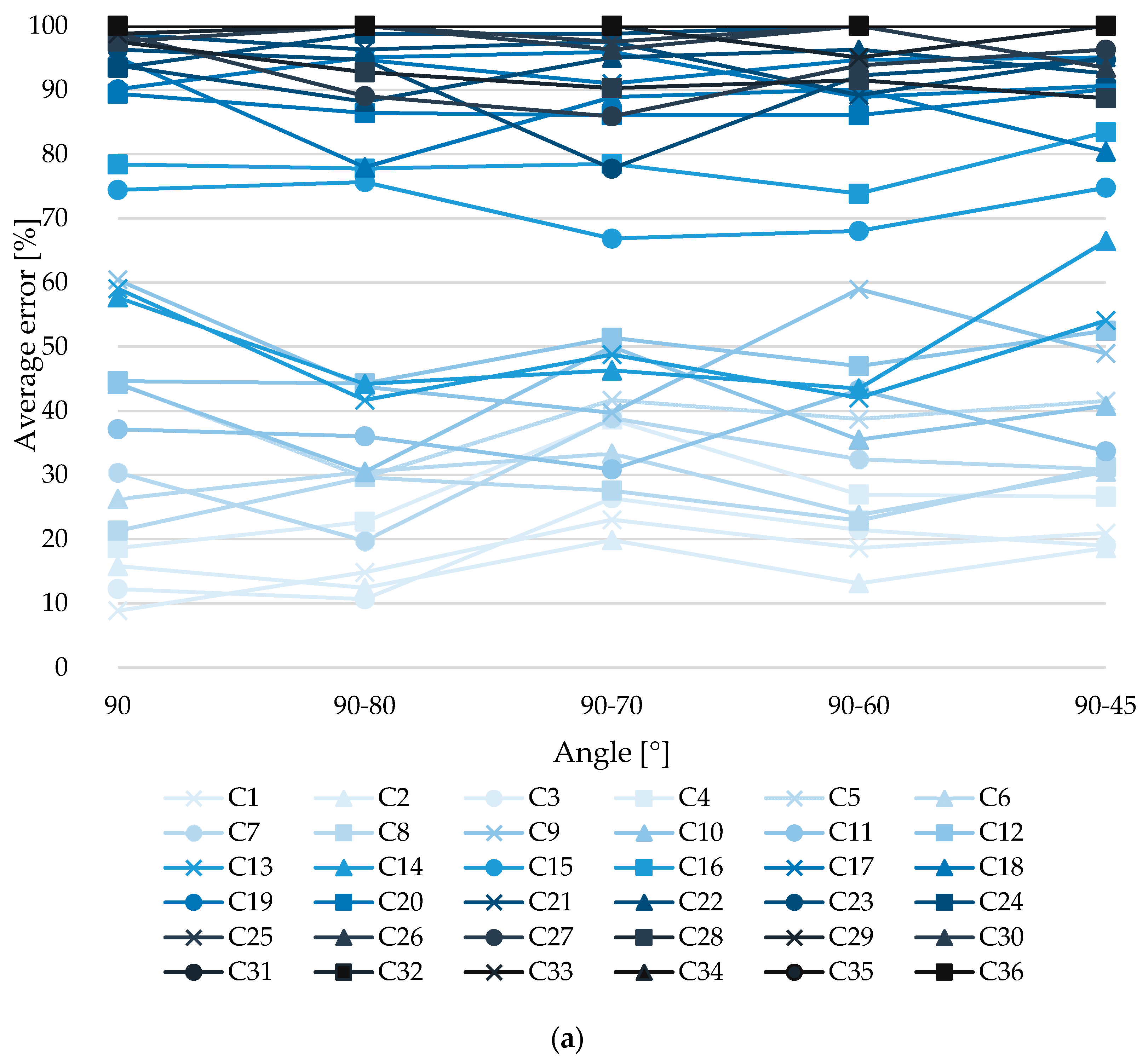
Figure 5, Figure 6 and Figure 7 show, respectively, the results of the experiment carried out. The horizontal axis corresponds to the variation or combination of camera angle for photo acquisition, while the vertical axis is the average error for potholes for depth (Figure 5), width (Figure 6), and volume (Figure 7). The sub-figures correspond to the different severity levels of each of these parameters: (a) low, (b) medium, and (c) high. On the other hand, the curves correspond to the different combinations in Table 3, starting with C1 (lighter color, lower height of photograph) to C36 (stronger color, the higher height of photograph). Thus, for each set of graphs, when the curves are located in the lower areas of each graph, it will represent that this combination Cn has a lower percentage of error in the measurement with the method used, with respect to its real value. On the other hand, those located in the upper part will have errors close to or equal to 100%; that is, in the latter case, it has not been possible to completely digitally reconstruct the pothole and the parameter of interest has not been measured.

Figure 5 displays the depth error values for each of the series, each including the variation and combination of camera angles for data acquisition. In Figure 5a, it is observed that the incorporation of an oblique angle in the acquisition of photographs produces lower error levels compared to models produced only with vertical photographs; more precisely, the reduction of error is 20%. Then, in Figure 5b,c the same behavior governs, i.e., the inclusion of an oblique angle decreases the error; however, for these severity levels (medium and high), the reduction of the error is much greater, on the order of 30%.

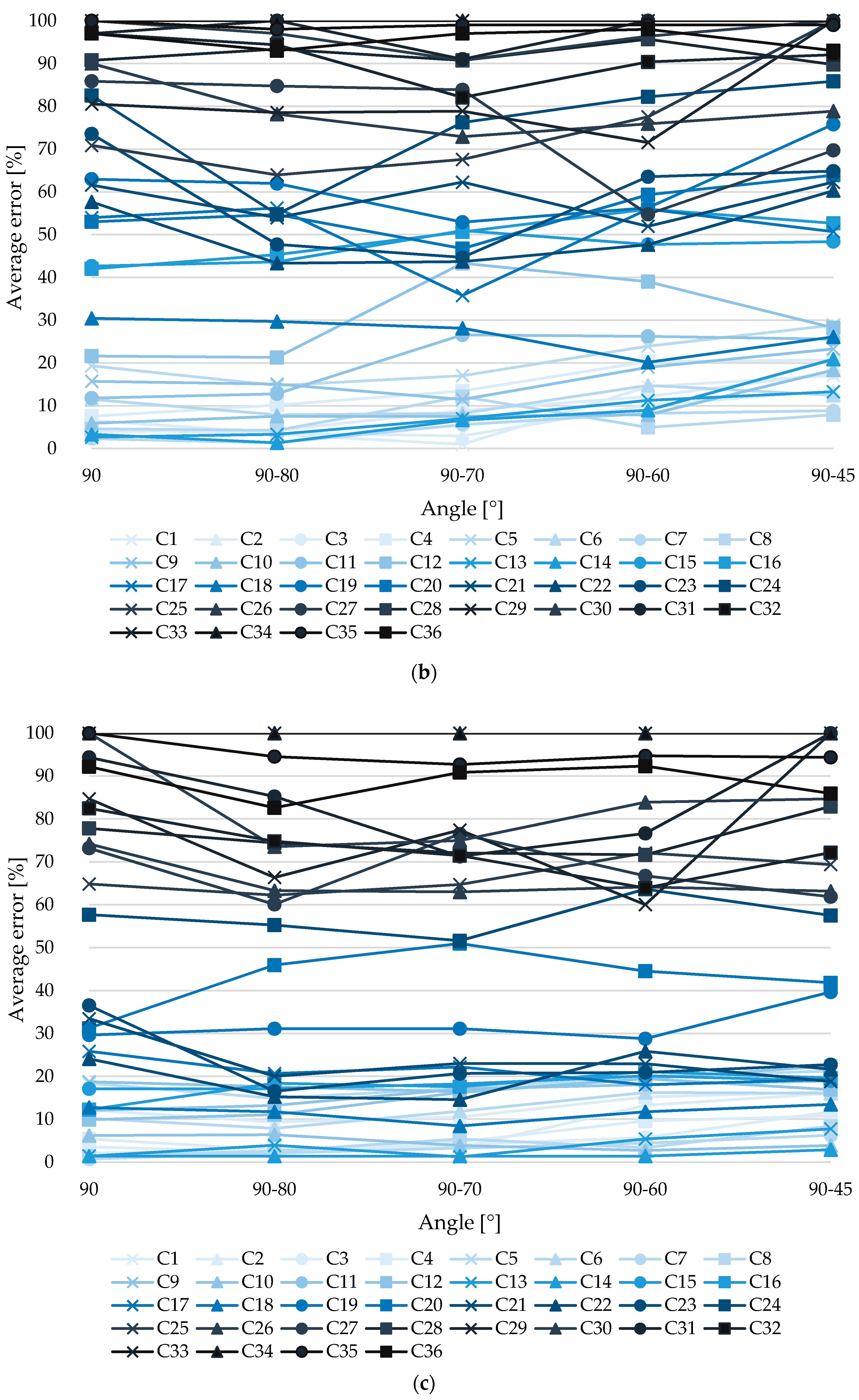
Figure 6 displays the width error values obtained from measuring the models of each series with different combinations and angle variations. In Figure 6, it is observed that for this case the inclusion of angle has a minimum impact (less than 2%) for cases with the least error, which are the relevant ones, since those manage to reliably measure the geometric characteristics of potholes. For higher height cases the reduction of the error when incorporating oblique angles is up to 60%, with errors around 50–60%.

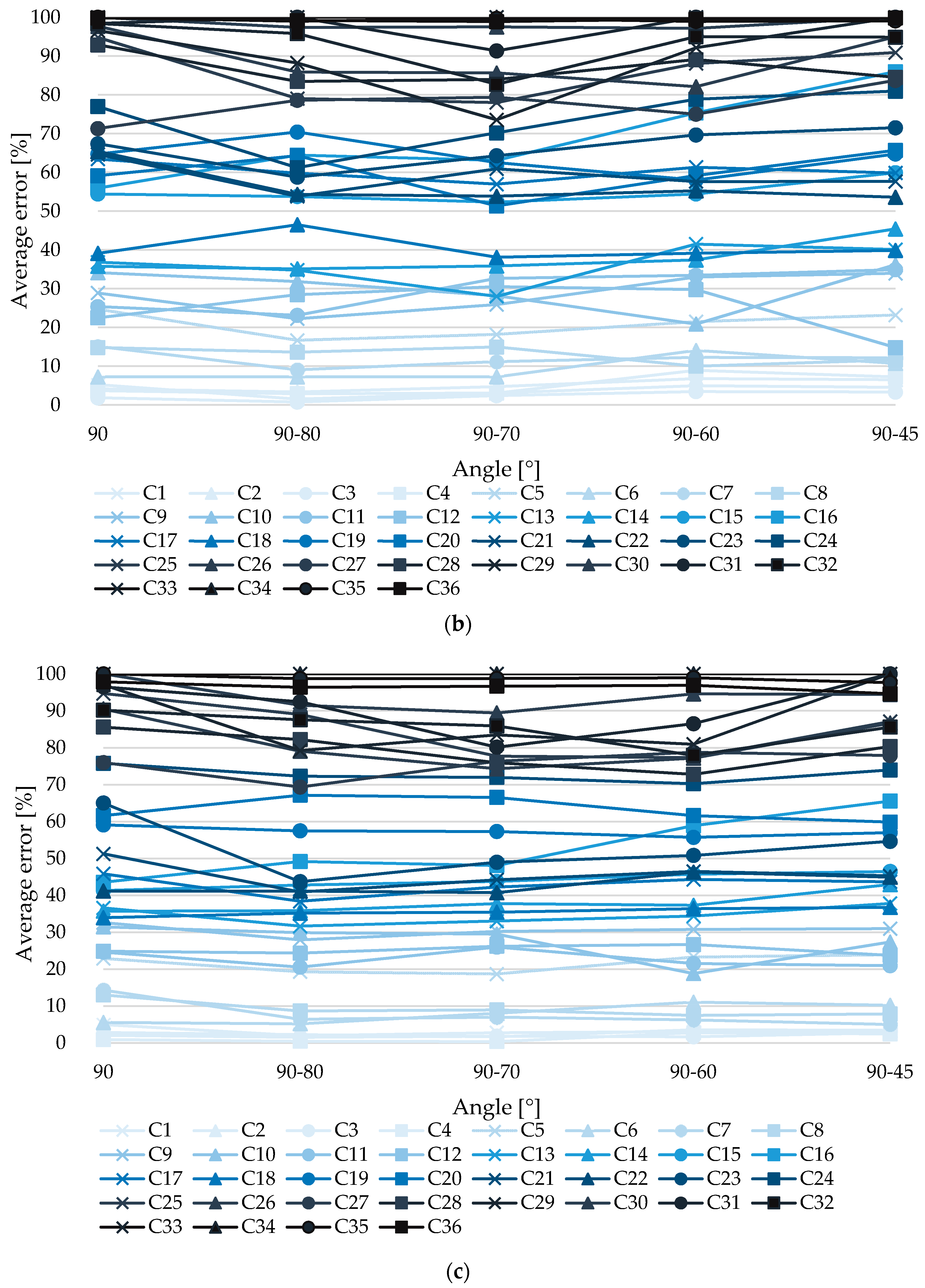
Figure 7 displays the volume error values, obtained from the measurement of the models of each series with combinations and angle variations. According to the figure, the horizontal axis is the variation or combination of camera angle for photo acquisition, while the vertical axis in Figure 7a–c is the average error of measuring pothole volume by severity level, low in Figure 7a, middle in Figure 7b and high in Figure 7c. In Figure 7, for the best case, the reduction from considering only the vertical angle (90°) is 39%.

The results indicate that the inclusion of angles other than 90° [–] have a positive impact on accuracy (error) for measuring the depth, width, and volume of potholes. However, this impact is low compared to the time-to-time effort to acquire this extra number of images, and the processing time is almost double. Likewise, there is no specific oblique angle or clear trend to ensure a reduction of the error. Therefore, working with vertical angles in this method remains the most efficient option for the acquisition of images with application in measurement of potholes on pavements, and in the same way remains consistent as a simple and fast method against more accurate technologies. Therefore, from now on, combinations with 90° angle will be discussed without any other variation or combination.

3.2. Variation in Overlap and Height

Figure 8 shows the values and behavior of the depth measurement error when varying height and overlap in vertical photo acquisition flights (90-degree camera angle) for different severity of potholes (low severity in Figure 8a, middle severity in Figure 8b and high severity in Figure 8c).

According to Figure 8a, it is observed that the error trend of all overlaps increases as the measurement height grows, which makes sense as the resolution of the photograph (GSD) decreases. In addition, the error variation decreases as the measurement height increases, indicating that errors converge due to their null interpretation, since the 100% error indicates that the variable to be measured in the model is not identified. On the other hand, there is no optimal overlap that applies to all of the heights. For 2 m, the best result was obtained for an overlap of 75%, with an error of 8.8%. For 5 m, the lowest error was 21.3% for a 90% overlap. For 8 m, the 85% overlap achieved the best results, resulting in an error of 37.1%. At 10 m, the minimum error was 57.7%, which is associated with an overlap of 80%, this error is 1.3% lower compared to an overlap of 75%, even more the error is reduced by more than 15% compared to overlaps of 85 and 90%. While, at 15 m, the 90% overlap has the lowest error (89.4%), an error that is 0.5% less compared to an overlap of 85%; moreover, the error is reduced by more than 5% compared to overlaps of 75 and 80%. However, the error is high (+89%). At 20 m, the least error (93.5%) was obtained with an overlap of 90%, the other overlaps had an error between 93.8–98.8%. At 25 m, there is a 100% error for the overlap of 80%, indicating that no depth could be measured for any of the potholes analyzed, while for overlaps of 75 and 90% the error is 87.5% for both and, for the overlap of 85%, an error of 98.8% was obtained. At 30 m, the overlaps of 80, 85 and 90% obtained a 100% error, which as stated above indicates that no depth was measured. Additionally, with the overlap of 75%, a 98.8% error was obtained, indicating that it was measured because the reconstruction of the 3D model created a slope in a pothole. At 40 m, all overlaps get an error of 100%, that is, no elevation was appreciated in the model; for this reason, the interpretation of the potholes in the model is like that of a circular horizontal dark spot. It can be observed that from 15 m that the error is high (about 90%) for the various overlaps, indicating that the analysis for higher heights is no longer representative for this type of measurement. However, it noted that the simulated potholes analyzed in the experiment would not present the same conditions in practice. In other words, since the experiment considers the value of width as twice the depth, due to its semi-spherical shape, it makes it a more conservative analysis, since the width of a pothole is much greater than its depth.

From Figure 8b, an optimal overlap is clearly observed for the heights of 2, 5, 8, 15, 20, 25 and 30 m, while, for the heights of 10 and 40 m, its optimum is not apparent at first sight. At 2 m, the least error was obtained (4%), four with an overlap of 85%; the other overlaps (75, 85 and 90%) have an error difference that exceeds 0.6% compared to the overlap of 75%. At 5 m, the optimal overlap is 85%, because with this overlap and height, the error is the lowest, specifically 2.3%; this error is 2.3% lower compared to an overlap of 90%. At 15 m, the least error was obtained (30.2%) with an overlap of 80%, the other overlaps (75, 85 and 90%) have an error difference that exceeds 22% compared to the overlap of 80%. At 8 m and 80% overlap, a 6% error was obtained, which is the lowest—5.9% lower compared to the 75% overlap. At 10 m, the optimal overlap is 75%, because with this overlap and height the error is the lowest, specifically 2.6%; this error is 0.6% lower compared to an overlap of 80%. Simultaneously, the error is reduced by more than 39% compared to the overlaps of 85 and 90%. At 15 m, the least error was obtained (30.2%) with an overlap of 80%, the other overlaps (75, 85 and 90%) has an error difference that exceeds 22% compared to the overlap of 80%. At 20 and 80% overlap, a 57% error was obtained, which is the lowest and is 4% lower compared to the 75% overlap; even better, the error is reduced by more than 15.8% compared to 85 and 90% overlaps. At 25 m the least error was obtained (70.2%) with an overlap of 75%, the other overlaps (80, 85 and 90%) have an error difference that exceeds 14.7%, compared to the overlap of 75%. At 30 m, the least error was obtained (79.6%) with an overlap of 75%, the other overlaps (80, 85 and 90%) have an error difference greater than 16.1% compared to the overlap of 75%. At 40 m, the error of all overlaps exceeds 95%, so the analysis is no longer representative. As mentioned in the previous analysis, the potholes analyzed would not have the same conditions as in practice (width >> depth), so the analysis remains conservative. Additionally, when looking at the same figure, the error of average severity potholes is reduced compared to low severity bumps, because their dimensions are larger.

From Figure 8c, an optimal overlap is observed for the heights of 8, 15, 20, 25 and 40 m, while, for the heights of 2, 5, 10 and 30 m its peak is not apparent at first sight. At 2 m, the least error was obtained (2.1%) with an overlap of 75%, the other overlaps (80, 85 and 90%) have an error difference greater than 1.5% compared to the overlap of 85%. For 5 m, the least error was obtained (0.7%) with an overlap of 85%, which has 0.7% less error compared to a 90% overlap. At 8 m, the least error (6.2%) was obtained with an overlap of 80%, which has 3.7% less error compared to an overlap of 90%. Simultaneously, the error is reduced by more than 5.9% compared to overlaps of 85 and 90%. At 10 m, the least error (1.4%) is for overlaps of 75 and 80%, the other overlaps (85 and 90%) have an error difference greater than 10.8% compared to overlaps of 75 and 80%. At 15 m, the least error was obtained (12.7%) with an overlap of 80%, the other overlaps (75, 85 and 90%) have an error difference greater than 13.1% compared to the overlap of 80%. At 20 m, the least error was obtained (24.1%) with an overlap of 80%, which has between 9.4% to 12.4% less error compared to an overlap of 75 and 85%. Moreover, the error is reduced more than 36.6% compared to the 90% overlap. At 25 m, the least error was obtained (64.8%) with an overlap of 75%, the other overlaps (80, 85 and 90%) have an error difference greater than 8.4% compared to the overlap of 75%. At 30 m, the least error was obtained (82.5%) with an overlap of 90%, which has 2.2% less error compared to an overlap of 75%, and at the same time, the error is reduced by more than 11.8% compared to the overlap of 85% and 17.5% compared to the overlap of 80%. At 40 m, the least error was obtained (92.2%) with an overlap of 90%, while for other overlaps (75, 80 and 85%) 100% errors were obtained, indicating that these measurements are no longer representative for this analysis. The potholes analyzed for high severity meet the conditions to be characterized as potholes, in the sense of their depth and width dimensions. However, it is important to be reminded that in practice the width is much larger than the depth, so the analysis remains conservative. Additionally, it is observed that the high severity bump error is reduced compared to the average severity potholes, because their dimensions are larger.

Figure 9 shows the values and behavior of the width measurement error when varying height and overlap in vertical photo acquisition flights (90-degree camera angle) for different severity of potholes (low severity in Figure 9a, middle severity in Figure 9b, high severity in Figure 9c).

According to Figure 9a and compared to the figure above, it is observed that the width measurement has a lower error than the bump depth measurement. At 2 m, the least error was obtained (3.6%) with an 80% overlap, which has 0.2% less error compared to the 85% overlap. At 5 m, the minimum error value (0.9%) was achieved with an overlap of 80%, which has between 1.4 and 2.3% less error compared to the other overlaps (75, 85 and 90%). For 8 m and an overlap of 80%, an error of 1.5% was found, which is the lowest for this height, comparing this error with respect to overlaps of 75 and 85% there is a difference between 2.3 and 3.5% less error respectively, even more, the error is reduced by 5.6% compared to an overlap of 90%. For 10 m, the least error was obtained (2.7%) with an overlap of 80%, which has 2.6% less error compared to an overlap of 75%, moreover, the error is reduced by more than 5.9% compared to overlaps of 85 and 90%. At 15 m, the least error (6.7%) it was obtained with an overlap of 80%, which has 5.7% less error compared to Z an overlap of 75%. Simultaneously, the error is reduced by more than 13.6% compared to overlaps of 85 and 90%. At 20 m, the variability of the error decreases compared to that obtained at 15 m. Additionally, for this height, the minimal error is obtained (16.2%) with an overlap of 80%, the other overlaps (75, 85 and 90%) have an error difference greater than 13.8% compared to the overlap of 80%. At 25 m, the error variation for the different overlaps decreases more compared to a height of 20 m. On the other hand, the least error (39.0%) was achieved with an overlap of 75%, which has 1.1% less error compared to an overlap of 80% and 4.4% less than the 90% overlap. Moreover, the error is reduced by 8.9% compared to an overlap of 85%. At 30 m, the least error was obtained (52.3%) with an overlap of 75%, for other overlaps (80, 85 and 90%) 100% errors were obtained, because the model did not rebuild potholes. At 40 m, all overlaps got 100% errors, which as mentioned earlier, is due to problems of modeling small bump sizes.

From Figure 9b, it is observed that the measurement of widths has less error than the measurement of bump depth. In addition, the error obtained is reduced compared to the analysis for low severity potholes. It is observed that up to a 30-m measuring height, the error does not exceed 20% for the different overlaps and at 40 m, error values greater than 45% are reached. At 2 m, the least error was obtained (1%) with an overlap of 80%, which has 0.6% less error compared to the overlap of 85%, while for an overlap of 75 and 90% the error is reduced by 1.4 to 1.1%. At 5 m, the minimum error value (0.5%) was obtained with an overlap of 75%, which has between 0.1 and 0.6% less error compared to the other overlaps (80, 85 and 90%). For 8 m and an overlap of 90%, an error of 1.1% was made. At 10 m, the least error was obtained (0.6%) with an overlap of 75 and 85%, the other overlaps (80 and 90%) have an error difference of 0.5% compared to overlaps of 75 and 85%. For 15 m, the least error (2.8%) was obtained with an overlap of 75%, which has 0.2% less error compared to overlaps of 80 and 90%. Moreover, the error is reduced by more than 5.9% compared to the overlap of 85%. At 20 m, the least error (3.5%) is obtained with an overlap of 80%, which is 1.2 and 1.3% less error compared to 90 and 75% overlaps respectively. The error is further reduced, up to 5.7% compared to the 85% overlap. For 25 m, the least error (6.9%) was obtained with an overlap of 80%, which has 1.9 and 2% less error compared to overlaps of 75 and 90%, respectively, while compared to the overlap of 85% the error is reduced by 7.1%. For 30 m, the least error was obtained (13.6%) with an overlap of 90%, which is between 2.3 and 3.1% less error compared to the other overlaps (75, 80 and 90%). At 40 m, the least error was obtained (47.0%) with an overlap of 85%, which has between 9 and 14% less error compared to the other overlaps (75, 80 and 90%).

From Figure 9c, it is observed that the measurement of widths has less error than the measurement of bump depth. The error obtained is reduced compared to the analysis for medium severity potholes. Additionally, note that for up to a 30-m measuring height, the error does not exceed 10.5% for the different overlaps and at 40 m, the overlap of 75% is the only one that exceeds 20% error, while the other overlaps do not exceed 14% error. At 2 m, the least error was obtained (0%) with an overlap of 80%, while for other overlaps the error was less than 1.6%. At 5 m, the minimum error value (0.5%) was obtained with an overlap of 80%, which has between 0.5 and 1% less error compared to the other overlaps (75, 85 and 90%). For 8 m and an overlap of 90%, an error of 0.3% was made, which is the lowest for this height, comparing this error with respect to overlaps of 75 and 80% there is a difference between 1.9 and 0.9% less error respectively, more so, the error is reduced by 2.7% compared to an overlap of 85%. At 10 m, the least error was obtained (0.3%) with an overlap of 80 and 85%, the other overlaps (70 and 90%) have an error difference of 0.4% compared to overlaps of 75 and 85%. At 15 m, the least error was obtained (0.8%) with an overlap of 80%, which has between 0.4 and 0.5% less error compared to overlaps of 90 and 75%, respectively, moreover, the error is reduced by 0.9% compared to the overlap of 85%. At 20 m, the least error is obtained with an overlap of 80%, which is 1.6% and is 0.3% lower compared to the overlap of 90%, moreover, the error is reduced by 1.5% to 2.4% compared to overlaps of 75 and 85%. At 25 m, the least error was obtained (2.8%) with an overlap of 80%, which is between 0.7 and 2.6% less error compared to the other overlaps (75, 85 and 90%). At 30 m, the least error was obtained (5.7%) with an overlap of 90%, which has 1.4% less error compared to an overlap of 80%. Moreover, the error is reduced by 4 to 4.3% compared to overlaps of 75 to 85%. At 40 m, the least error was obtained (11.4%) with an overlap of 90%, which has 1.8% less error compared to overlaps of 80 and 85%. Moreover, the error is reduced by 11.5% compared to an overlap of 75%.

Figure 10 shows the values and behavior of the volume measurement error by varying the height and overlap in vertical photo acquisition flights (90-degree camera angle) for different severity in potholes (low severity in Figure 10a, middle severity in Figure 10b, high severity in Figure 10c).

In Figure 10a, a trend is observed of overlapping error increases as the measurement height grows. On the other hand, it is observed that the error at 10 m is greater than 60% for all overlaps, indicating that the experiment does not work well for this type of analysis. At 2 m, the minimum error was 4.1%, which is associated with an overlap of 80%, this error is 2% lower compared to an overlap of 85%, even more the error is reduced by more than 3.6% compared to overlaps of 75 and 90%. At 5 m, the 80% overlap has the lowest error (6.4%), an error that is 9.2% less compared to an overlap of 85%. Moreover, the error is reduced by more than 9.4% compared to 75 and 90% overlaps. At 8 m, the least error (36.6%) was obtained with a 90% overlap. For 10 m and with an overlap of 75% an error of 63.1% was obtained, which is the lowest for this height, since it has 5.5% less error compared to the overlap of 80%. Moreover, the error is reduced by 12.8 to 18.7% compared to the overlaps of 85 and 90%. At 15 m, the least error was obtained (81.9%) with an overlap of 90%, which is between 2.9 and 10.1% less error compared to the other overlaps (75, 80 and 85%). At 20 m, the error is 95% for an 80% overlap, which is high for further analysis of this type of measurement. So, from 20 m, an analysis of volume for low severity potholes loses value in practice, since the volume of the pothole fails to describe a semi-sphere, but rather tries to reconstruct a kind of cone, from the position in which the maximum depth was obtained. The behavior is similar to that observed in the pothole depth analyses, as the measured volume depends directly on how good the measurement has been with respect to depth and area characteristics.

From Figure 10b, a trend is observed of overlapping error increases as the capture height grows. On the other hand, it is observed that the error at 10 m is greater than 30% for overlaps of 75 and 80% and more than 50% for overlaps of 85 and 90%, indicating that the experiment does not work properly for this type of analysis. However, the error is reduced from what was observed in the previous analysis. At 2 m, the minimum error was 1.9%, which is associated with an overlap of 85%, this error is 1.8% lower compared to an overlap of 90%, even more so the error is reduced by more than 2.3% compared to overlaps of 75 and 80%. At 5 m, the 80% overlap has the lowest error (7.3%), an error that is 7.5% less compared to a 90% overlap. Moreover, the error is reduced by more than 7.8% compared to 75 and 85% overlaps. At 8 m, the least error (22.5%) was obtained with a 90% overlap. At 10 m, the least error was obtained (35.8%) with an overlap of 80%, which has 1% less error compared to the overlap of 75%, while for an overlap of 85 and 90% the error is reduced by 18.6 to 20.1%. At 15 m, the minimum error value (39.1%) was obtained with an overlap of 80%, which has between 20.0 and 25.6% less error compared to the other overlaps (75, 85 and 90%). For 20 m and an overlap of 75%, an error of 64.6% was produced, which is the lowest for this height, comparing this error with respect to overlaps of 80 and 85% there is a difference between 0.8 and 2.8% less error respectively, more than that, the error is reduced by 11.6% compared to an overlap of 90%. At 25 m, the least error was obtained (71.3%) for an 85% overlap, which is between 21.6 and 26.4% less error compared to other overlaps (75, 80 and 90%). At 30 m, the error obtained was 96.5% for an overlap of 75%, which is the lowest and at the same time high considering its magnitude, so it loses practical value. At 40 m, the error is higher than that obtained at a height of 30 m. From the above it is observed that from 30 m it loses practical value.

From Figure 10c, a trend is observed of overlapping error increasing as the capture height grows. However, at 15 m with an overlap of 80%, the volume obtained was 1.8% lower than that obtained at 10 m with the same overlap. This is probably explained by problems in rebuilding with the software. On the other hand, it is observed that the error is similar to that made in the previous analysis, since at 10 m the error is greater than 30% for overlaps of 75 and 80% and more than 40% for overlaps of 85 and 90%, indicating that the experiment does not work properly for this type of analysis. At 2 m, the minimum error was 0.9%, which is associated with a 90% overlap, this error is 1.2% lower compared to an overlap of 85%, even more so the error is reduced by more than 1.9% compared to overlaps of 75 and 80%. At 5 m, the 80% overlap has the lowest error (5.5%), an error that is 7.5% less compared to a 90% overlap. Moreover, the error is reduced by more than 8.8% compared to 75 and 85% overlaps. At 8 m, the least error (24.6%) was obtained with an overlap of 85%. At 10 m, the least error was obtained (35.7%) with an overlap of 80%, which has 0.9% less error compared to the overlap of 75%. Moreover, the error is reduced by 5.6 to 7.8% compared to overlaps of 85 and 90%. At 15 m, and with an overlap of 80% an error of 33.9% was obtained, which is the lowest for that height, and which is 11.9% lower compared to the overlap of 75%. Moreover, the error is reduced by 25.2 to 27.7% compared to overlaps of 85 and 90%. For 20 m, the lowest error is 41.2%, which is associated with an 80% overlap, and has 10% less error compared to an overlap of 75%. Moreover, the error is reduced by 23.8 to 34.6% compared to overlaps of 85 and 90%. At 25 m, the least error was obtained (75.9%) with an 85% overlap, which is between 9.7 and 18.8% less error compared to the other overlaps (75, 80 and 90%). At 30 m, the minimum error (90.2%) was held for an overlap of 90%, which has no practical value. At 40 m, the error is high with respect to the value obtained at a height of 30 m. For the overlaps of 75, 80 and 85%, the volume could not be measured because no depth was recorded.

3.3. Selecting Optimal Parameters

From the selection by geometric characteristic type, i.e., width, depth, and bump volume, the overall combination that allows for the most reliable results must be selected, since the characteristics of potholes in a real application will be determined by a single model. In this way, optimal recommendations in depth, width and volume measurements were analyzed, always seeking to minimize the error of these types of measurement.

Table 4. Recommended overlap by height associated with severity level of interest to be measured; p is longitudinal overlap and q is transverse overlap.

Height [m]	p [%]	q [%]	Severity	Wide Error [%]	Depth Error [%]	Volume Error [%]
2	80	72	Low	3.6	15.8	4.1
	85	77	Middle	1.6	4.0	1.9
	75	68	High	1.6	2.1	5.0
5	80	72	Low	0.9	26.2	6.4
	80	72	Middle	1.1	11.6	7.3
	80	72	High	0.5	10.2	5.5
8	80	72	Low	1.5	44.2	48.6
	80	72	Middle	4.5	6.0	34.1
	80	72	High	1.24	6.2	31.5
10	80	72	Low	2.7	57.7	68.6
	75	68	Middle	0.6	2.6	36.8
	80	72	High	0.3	1.4	35.7
15	80	72	Low	6.7	95.1	84.8
	80	72	Middle	3	30.2	39.1
	80	72	High	0.8	12.7	33.9
20	80	72	Low	16.2	93.8	95
	80	72	Middle	3.5	57	65.4
	80	72	High	1.6	24.1	41.2
25	75	68	Low	39	64.8	99.5
	75	68	Middle	8.93	70.2	94.8
	75	68	High	5.4	64.8	94.7
30	75	68	Low	52.3	98.8	99.4
	75	68	Middle	16.5	79.6	96.5
	90	81	High	5.7	82.5	90.2
40	-	-	Low	-	-	-
	85	77	Middle	47	99	100
	90	81	High	11.4	92.2	97.8

was based on the discussion presented in Section 3.2, the recommended overlap was chosen by severity level, as the use of these recommendations varies depending on the minimum level of severity to be measured. For heights of 2, 5 and 8 m, the experiments were excessively laborious. For these heights, it is difficult to ensure proper positioning and correct overlap between images, as the handling of the UAV at such a low height becomes imprecise due to the sensitivity of the control. In addition, the GPS does not deliver a correct position of the aircraft, which in some cases led to the necessary repetition of the shooting. Although capturing photographs at low altitude allows for more accurate 3D models, in practical terms and in order to optimize the flight and inspection (balance in time, quality, area observed, etc.), it is not recommended to perform the flights at the indicated heights. Therefore, it is not recommended to plan flights with heights less than 10 m. At 40 m, the error levels are maximum, therefore there is no practical justification to make a recommendation for this. For the realization of the case study, the height recommendations of 10 and 15 m were used, which present an acceptable level of error in practice.

Table 5. Recommended distances to meet optimal height overlap. (a) p = 75, q = 68 [%]; (b) p = 80, q = 72 [%]; (c) p = 85, q = 77 [%]; (d) p = 90, q = 81 [%].

(a)
Height [m]/GSD [cm/pixel]	Overlap; p = 75 y q = 68 [%]
	B [m]	A [m]
2/0.05	0.5	0.9
5/0.13	1.2	2.3
8/0.21	1.9	3.7
10/0.27	2.4	4.7
15/0.40	3.6	7.0
20/0.53	4.9	9.3
25/0.67	6.1	11.7
30/0.80	7.3	14.0
40/1.07	9.7	18.7
(b)
Height [m]/GSD [cm/pixel]	Overlap; p = 80 y q = 72 [%]
	B [m]	A [m]
2/0.05	0.4	0.8
5/0.13	1.0	2.0
8/0.21	1.6	3.3
10/0.27	1.9	4.1
15/0.40	2.9	6.1
20/0.53	3.9	8.2
25/0.67	4.9	10.2
30/0.80	5.8	12.2
40/1.07	7.8	16.3
(c)
Height [m]/GSD [cm/pixel]	Overlap; p = 85 y q = 77 [%]
	B [m]	A [m]
2/0.05	0.3	0.7
5/0.13	0.7	1.7
8/0.21	1.2	2.7
10/0.27	1.5	3.4
15/0.40	2.2	5.0
20/0.53	2.9	6.7
25/0.67	3.6	8.4
30/0.80	4.4	10.1
40/1.07	5.8	13.4
(d)
Height [m]/GSD [cm/pixel]	Overlap; p = 90 y q = 81 [%]
	B [m]	A [m]
2/0.05	0.2	0.6
5/0.13	0.5	1.4
8/0.21	0.8	2.2
10/0.27	1.0	2.8
15/0.40	1.5	4.2
20/0.53	1.9	5.5
25/0.67	2.4	6.9
30/0.80	2.9	8.3
40/1.07	3.9	11.1

shows longitudinal (B) and transverse distances (A) between photographs captured with the UAV to comply with overlaps; longitudinal (p) and transverse (q) for each of the heights.

These distances are used to calculate the flight lines needed to fully cover the pavement unit to be inspected. To know the number of flight lines for a given road width, Equation (1) should be used. An additional line is added to ensure full width coverage. Additionally, to have a reference of the number of photographs to be taken per flight line, it is recommended to use Equation (2). Four additional photos are added, two for the start and two for the end of the flight line, in order to have the ends properly overlapped. Naturally, the corners will have a lower number of photo coverage compared to the center, as can be seen in an example in Figure 11. That is necessary to guarantee a minimum of photographs in the corners of the pavement to have all the areas covered on the map.

$$Flightline[\#]=\frac{Poadwidth\left[m\right]}{A\left[m\right]}+1$$

(1)

$$Photographyperflightline[\#]=\frac{Pavementlenght\left[m\right]}{B\left[m\right]}+4$$

(2)

3.4. Case Study

A study is carried out a real case study to validate whether recommendations can be extrapolated in the measurement of bumps of deteriorated asphalt pavements. The actual pavement section has 6 potholes with different dimensions (indicated in the

Table 6. Dimensions of potholes measured in terrain (real).

Pothole	Smaller Width [mm]	Larger Width [mm]	Depth [mm]	Volume [cm3]
(a)	360	545	50	7150.35
(b)	380	740	73	14,257.27
(c)	300	870	70	9976.74
(d)	345	833	74	15,112.24
(e)	260	355	40	1245.14
(f)	170	570	30	2341.34

. Flexible pavement pothole for recommendation validation.

Figure 12 shows the potholes by indicating by a horizontal arrow the largest width and a vertical arrow the smallest width.

The first analysis was carried out at a height of 10 [m] applying the recommendations detailed above. The results are shown in

Table 7. Dimensions of potholes measured in model at 10 m and error.

Pothole	Width [mm]	Error [%]	Depth [mm]	Error [%]	Volume [cm3]	Error [%]	Severity
(a)	540	0.9	45	10	4712.84	34.1	Middle
(b)	736	0.5	66	9.6	11,255.31	21.1	High
(c)	860	1.1	66	5.7	7365.53	26.2	High
(d)	829	0.5	70	5.4	9751.60	35.5	High
(e)	350	1.4	38	5	1007.30	19.1	Middle
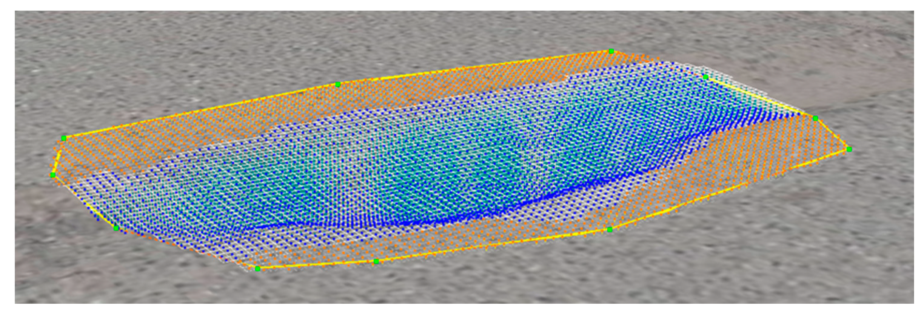
(f)	566	0.7	27	10	1701.04	27.3	Low

, in addition to Figure 13, where the reconstruction of a pothole in the case study can be observed.

The second analysis went to one of 15 [m], the results are shown in

Table 8. Dimensions of potholes measured in model at 15 m and error.

Pothole	Width [mm]	Error [%]	Depth [mm]	Error [%]	Volume [cm3]	Error [%]	Severity
(a)	537	1.5	44	12	4812.26	32.7	Middle
(b)	732	1.1	63	13.7	11,346.65	20.4	High
(c)	864	0.7	64	8.6	7578.54	24	High
(d)	824	1.1	65	12.2	9641.74	36.2	High
(e)	348	2	35	12.5	987.47	20.7	Middle
(f)	564	1.1	27	10	1814.25	22.5	Low

.

It is important to note that potholes were marked for case study planning in order to clearly identify the measured points in the field, in order to minimize the measurement error of the evaluator.

For the analysis at 10 m, the measurements of the height and width were obtained with high accuracy, compared to the other measurement variables, since with the help of the marks, these characteristics could be better determined. However, for depth measurement, the error was greater, with the worst case being 9.9% higher than the value of the recommendation; this can be explained by the irregular shape of the bumpy surface, i.e., the surface is not completely horizontal. However, the measurement error could be obtained with high accuracy (error less than 1 cm). On the other hand, the volume analysis presented a similar error with respect to the value of the recommendation. However, it remains a high error to consider it as a potential variable to be measured with this method.

For the 15 m height analysis, the width measurement was greater than the values obtained at 10 m, although for the pothole (c) a difference of 0.4% was presented. This is probably explained by the variability of measurement in terrain and the sensitivity of the study variable, which for a millimeter error in the measurement results in the error percentage presenting an atypical or unexpected behavior. In the measurement of depth and volume, the error behaved better than expected (according to the results of the study surface) which can be explained by the fact that these potholes have a large surface with respect to their depth; this certainly helps to rebuild the volume and obviously the depth.

As the above results demonstrate, the recommendations allow for a good measure of the geometric characteristics of pavement potholes. The level of error is about one centimeter, which is a promising methodology applied to the regular practice of engineering.

4. Conclusions

The literature review process allowed us to gather a history of the use of UAVs as a tool for data acquisition. This tool is positioned as an economical substitute compared to more sophisticated emerging technologies, such as the terrestrial laser scanner, used for pavement inspection. It also served as the basis for developing a workflow for photo acquisition and further processing using the SfM–MVS technique. It also understands the importance of variables that influence flight planning.

This research focused on developing a practical method for measuring geometric characteristics of potholes, using 3D models generated with photographs acquired with a UAV and processed through software based on the SfM–MVS technique. To develop this methodology, an experiment was conducted to evaluate the accuracy in the reconstruction of 3D models using images obtained from the variation and combination of different parameters of flight planning and data capture (digital photographs). Specifically, variations in the combinations of camera angles (vertical–oblique), image overlaps and flight height.

The experiment concludes that the incorporation of oblique photographs into a set of vertical photographs does not guarantee a significant reduction in error. Therefore, the research focused on error assessment for different combinations of height and overlap with vertical angle of photo acquisition. Within the geometric characteristics of the pavement studied, the width is the characteristic that has the lowest level of error, followed by depth and last by volume.

After the evaluation of the error, both for depth, width and volume, practical recommendations were generated according to the level of severity of potholes. It was obtained that the methodology is applicable for heights of 10 to 15 m, since at higher heights the error levels do not allow to represent well the characteristics sought, while at lower heights the process becomes extremely laborious when having to perform manual flights; additionally, the GPS becomes sensitive and imprecise at these heights. These recommendations were validated in a real case study, demonstrating that they are extrapolatable to the regular practice of engineering, specifically, in the inspection of asphalt pavements.

The future work of this research should focus on improving the accuracy of the models generated by incorporating ground control points (GCPs), mainly to apply it on road pavements that have milestones or benchmarks that are accessible prior to the acquisition of photographs. The GCPs improve accuracy because they are the first mooring points that improve relative accuracy levels while increasing the absolute position of the model. Moreover, another line of research could include the automatic extraction of characteristics of pavement models generated by SfM–MVS in conjunction with photographs acquired based on the recommendations of this research.

References

1. Agnisarman, S.; Lopes, S.; Chalil Madathil, K.; Piratla, K.; Gramopadhye, A. A survey of automation-enabled human-in-the-loop systems for infrastructure visual inspection. Autom. Constr. 2019, 97, 52–76. [Google Scholar] [CrossRef]
2. Okine, A.; Adarkwa, O. Pavement Condition Surveys—Overview of Current Practices; University of Delaware: Newark, DE, USA, 2013. [Google Scholar]
3. Zhang, L.; Xu, W.; Zhu, L.; Yuan, X.; Zhang, C. Study on pavement defect detection based on image processing utilizing UAV. J. Phys. Conf. Ser. 2019, 1168, 042011. [Google Scholar] [CrossRef]
4. Bar-Hillel, A.; Lerner, R.; Levi, D.; Raz, G. Recent progress in road and lane detection: A survey. Mach. Vis. Appl. 2014, 25, 727–745. [Google Scholar] [CrossRef]
5. Liu, P.; Chen, A.; Huang, Y.; Han, J.; Lai, J.; Kang, S.; Wu, T.; Wen, M.; Tsai, M. A review of rotorcraft unmanned aerial vehicle (UAV) developments and applications in civil engineering. Smart Struct. Syst. 2014, 13, 1065–1094. [Google Scholar] [CrossRef]
6. Peffers, K.; Tuunanen, T.; Gengler, C.; Rossi, M.; Hui, W.; Virtanen, V.; Bragge, J. The design science research process: A model for producing and presenting information systems research. In Proceedings of the 1st International Conference on Design Science Research in Information Systems and Technology (DESRIST 2006), Claremont, CA, USA, 24–25 February 2006. [Google Scholar]
7. Peffers, K.; Tuunanen, T.; Rothenberger, M.A.; Chatterjee, S. A design science research methodology for information systems research. J. Manag. Inf. Syst. 2007, 45–77. [Google Scholar] [CrossRef]
8. Walls, J.; Widmeyer, G.; El-Sawy, O. Building an information system design theory for vigilant EIS. Inf. Syst. Res. 1992, 3, 36–59. [Google Scholar] [CrossRef]
9. Hevner, A.; March, S.; Park, J. Design research in information systems research. MIS Q. 2004, 28, 75–105. [Google Scholar] [CrossRef] [Green Version]
10. Branco, L.H.C.; Segantine, P.C.L. MaNIAC-UAV: A methodology for automatic pavement defects detection using images obtained by Unmanned Aerial Vehicles. J. Phys. Conf. Ser. 2015, 633, 012122. [Google Scholar] [CrossRef]
11. Knyaz, V.A.; Chibunichev, A.G. Photogrammetric techniques for road surface analysis. Int. Arch. Photogramm. Remote Sens. Spat. Inf. Sci. 2016, 41, 515–520. [Google Scholar] [CrossRef]
12. Miller, J.; Bellinger, W. Distress Identification Manual for the Long-Term Pavement Performance Program; United States Federal Highway Administration, Office of Infrastructure Research and Development: Washington, DC, USA, 2014; Volume 129.
13. Haas, R.; Hudson, W.R.; Falls, L.C. Pavement Asset Management; Wiley Publisher: Hoboken, NJ, USA, 2015. [Google Scholar]
14. Zhang, S.; Lippitt, C.D.; Bogus, S.M.; Neville, P.R.H. Characterizing pavement surface distress conditions with hyper-spatial resolution natural color aerial photography. Remote Sens. 2016, 8, 392. [Google Scholar] [CrossRef] [Green Version]
15. Cheng, H.D.; Miyojim, M. Automatic pavement distress detection system. J. Comput. Civ. Eng. 1998, 12, 145–152. [Google Scholar] [CrossRef]
16. Zakeri, H.; Nejad, F.M.; Fahimifar, A. Rahbin: A quadcopter unmanned aerial vehicle based on a systematic image processing approach toward an automated asphalt pavement inspection. Autom. Constr. 2016, 72, 211–235. [Google Scholar] [CrossRef]
17. Wang, K.C.P.; Li, X. Use of digital cameras for pavement surface distress survey. Transp. Res. Rec. 1999, 1675, 91–97. [Google Scholar] [CrossRef]
18. Wang, K.C.P.; Smadi, O. Automated Imaging Technologies for Pavement Distress Surveys; Transportation Research Board of Research Academies: Washington, DC, USA, 2011. [Google Scholar]
19. McGhee, K.H. Automated pavement distress collection techniques. Autom. Pavement Distress Collect. Tech. 2004. [Google Scholar] [CrossRef]
20. Wang, K.C.P.; Elliott, R.P. Investigation of Image Archiving for Pavement Surface Distress Survey; University of Arkansas: Fayetteville, NC, USA, 1999. [Google Scholar]
21. Ersoz, A.B.; Pekcan, O.; Teke, T. Crack identification for rigid pavements using unmanned aerial vehicles. Proc. IOP Conf. Ser. Mater. Sci. Eng. 2017, 236. [Google Scholar] [CrossRef]
22. Li, Q.; Zou, Q.; Zhang, D.; Mao, Q. FoSA: F* Seed-growing Approach for crack-line detection from pavement images. Image Vis. Comput. 2011, 29, 861–872. [Google Scholar] [CrossRef]
23. Wang, X.; Feng, X. Pavement distress detection and classification with automated image processing. In Proceedings of the International Conference on Transportation, Mechanical, and Electrical Engineering (TMEE), Changchun, China, 16–18 December 2011; Volume 2006, pp. 1345–1350. [Google Scholar]
24. Xu, B.; Huang, Y. Automatic inspection of pavement cracking distress. Appl. Digit. Image Process. 2005, 5909. [Google Scholar] [CrossRef]
25. Oliveira, H.; Correia, P.L. Automatic road crack detection and characterization. IEEE Trans. Intell. Transp. Syst. 2013, 14, 155–168. [Google Scholar] [CrossRef]
26. Zou, Q.; Cao, Y.; Li, Q.; Mao, Q.; Wang, S. CrackTree: Automatic crack detection from pavement images. Pattern Recognit. Lett. 2012, 33, 227–238. [Google Scholar] [CrossRef]
27. Nguyen, T.S.; Avila, M.; Begot, S. Automatic detection and classification of defect on road pavement using anisotropy measure. In Proceedings of the European Signal Processing Conference, Glasgow, UK, 24–28 August 2009; pp. 617–621. [Google Scholar]
28. Ragnoli, A.; De Blasiis, M.; Di Benedetto, A. Pavement distress detection methods: A review. Infrastructures 2018, 3, 58. [Google Scholar] [CrossRef] [Green Version]
29. Kumar, P.; Angelats, E. An automated road roughness detection from mobile laser scanning data. Int. Arch. Photogramm. Remote Sens. Spat. Inf. Sci. 2017, 42, 91–96. [Google Scholar] [CrossRef] [Green Version]
30. Barbarella, M.; D’Amico, F.; De Blasiis, M.R.; Di Benedetto, A.; Fiani, M. Use of terrestrial laser scanner for rigid airport pavement management. Sensors 2018, 18, 44. [Google Scholar] [CrossRef] [PubMed] [Green Version]
31. Barbarella, M.; De Blasiis, M.R.; Fiani, M. Terrestrial laser scanner for the analysis of airport pavement geometry. Int. J. Pavement Eng. 2019, 20, 466–480. [Google Scholar] [CrossRef]
32. Inzerillo, L.; Di Mino, G.; Roberts, R. Image-based 3D reconstruction using traditional and UAV datasets for analysis of road pavement distress. Autom. Constr. 2018, 96, 457–469. [Google Scholar] [CrossRef]
33. Tan, Y.; Li, Y. UAV Photogrammetry-based 3D road distress detection. ISPRS Int. J. Geo-Inf. 2019, 8, 409. [Google Scholar] [CrossRef] [Green Version]
34. Congress, S.S.C.; Puppala, A.J.; Lundberg, C.L. Total system error analysis of UAV-CRP technology for monitoring transportation infrastructure assets. Eng. Geol. 2018, 247. [Google Scholar] [CrossRef]
35. Díaz-Vilariño, L.; González-Jorge, H.; Martínez-Sánchez, J.; Bueno, M.; Arias, P. Determining the limits of unmanned aerial photogrammetry for the evaluation of road runoff. Meas. J. Int. Meas. Confed. 2016, 85, 132–141. [Google Scholar] [CrossRef]
36. Leonardi, G.; Barrile, V.; Palamara, R.; Suraci, F.; Candela, G. 3D mapping of pavement distresses using an Unmanned Aerial Vehicle (UAV) system. Smart Innov. Syst. Technol. 2019, 101, 164–171. [Google Scholar]
37. Liu, D.; Chen, J.; Hu, D.; Zhang, Z. Dynamic BIM-augmented UAV safety inspection for water diversion project. Comput. Ind. 2019, 108, 163–177. [Google Scholar] [CrossRef]
38. Pan, Y.; Zhang, X.; Cervone, G.; Yang, L. Detection of Asphalt Pavement Potholes and Cracks Based on the Unmanned Aerial Vehicle Multispectral Imagery. IEEE J. Sel. Top. Appl. Earth Obs. Remote Sens. 2018, 11, 3701–3712. [Google Scholar] [CrossRef]
39. Zhang, C.; Elaksher, A. An unmanned aerial vehicle-based imaging system for 3D measurement of unpaved road surface distresses. Comput. Civ. Infrastruct. Eng. 2012, 27, 118–129. [Google Scholar] [CrossRef]
40. Henrickson, J.V.; Rogers, C.; Lu, H.H.; Valasek, J.; Shi, Y. Infrastructure assessment with small unmanned aircraft systems. In Proceedings of the International Conference on Unmanned Aircraft Systems (ICUAS), Arlington, VA, USA, 8 June 2016; pp. 933–942. [Google Scholar]
41. Aldea, E.; Le Hégarat-Mascle, S. Robust crack detection for unmanned aerial vehicles inspection in an a-contrario decision framework. J. Electron. Imaging 2015, 24, 061119. [Google Scholar] [CrossRef] [Green Version]
42. Bemis, S.P.; Micklethwaite, S.; Turner, D.; James, M.; Akciz, S.; Thiele, S.; Bangash, H. Ground-based and UAV-Based photogrammetry: A multi-scale, high-resolution mapping tool for structural geology and paleoseismology. J. Struct. Geol. 2014, 69, 163–178. [Google Scholar] [CrossRef]
43. Lowe, D.G. Distinctive image features from scale-invariant keypoints. Int. J. Comput. Vis. 2004, 60, 91–110. [Google Scholar] [CrossRef]
44. Furukawa, Y.; Ponce, J. Accurate, dense, and robust multiview stereopsis. IEEE Trans. Pattern Anal. Mach. Intell. 2010, 32, 1362–1376. [Google Scholar] [CrossRef]
45. Mikolajczyk, K.; Tuytelaars, T.; Schmid, C.; Zisserman, A.; Matas, J.; Schaffalitzky, F.; Kadir, T.; Van Gool, L. A comparison of affine region detectors. Int. J. Comput. Vis. 2005, 65, 43–72. [Google Scholar] [CrossRef] [Green Version]
46. Szeliski, R. Computer Vision: Algorithms and Applications; Springer: Berlin, Germany, 2004. [Google Scholar]
47. Turner, D.; Lucieer, A.; Wallace, L. Direct georeferencing of ultrahigh-resolution UAV imagery. IEEE Trans. Geosci. Remote Sens. 2014, 52, 2738–2745. [Google Scholar] [CrossRef]
48. Quirós, E. Introducción a la Fotogrametría y Cartografía Aplicadas a la Ingeniería Civil; Universidad de Extremadura: Cáceres, España, 2014. [Google Scholar]
49. Martin, R.A.; Rojas, I.; Franke, K.; Hedengren, J.D. Evolutionary view planning for optimized UAV terrain modeling in a simulated environment. Remote Sens. 2016, 8, 26. [Google Scholar] [CrossRef] [Green Version]
50. James, M.R.; Robson, S. Mitigating systematic error in topographic models derived from UAV and ground-based image networks. Earth Surf. Process. Landf. 2014, 39, 1413–1420. [Google Scholar] [CrossRef] [Green Version]
51. James, M.R.; Robson, S.; d’Oleire-Oltmanns, S.; Niethammer, U. Optimising UAV topographic surveys processed with structure-from-motion: Ground control quality, quantity and bundle adjustment. Geomorphology 2017, 280, 51–66. [Google Scholar] [CrossRef] [Green Version]
52. Nesbit, P.R.; Hugenholtz, C.H. Enhancing UAV-SfM 3D model accuracy in high-relief landscapes by incorporating oblique images. Remote Sens. 2019, 11, 239. [Google Scholar] [CrossRef] [Green Version]
53. Micheletti, N.; Chandler, J.H.; Lane, S.N. Structure-from-motion photogrammetry. GIM Int. 2017, 31, 36–39. [Google Scholar]
54. Pix4D. How to Verify that There is Enough Overlap between the Images. 2019. Available online: https://support.pix4d.com/hc/en-us/articles/203756125-How-to-verify-that-there-is-enough-overlap-between-the-images (accessed on 3 January 2020).
55. Goodbody, T.R.H.; Coops, N.C.; White, J.C. Digital Aerial photogrammetry for updating area-based forest inventories: A review of opportunities, challenges, and future directions. Curr. Rep. 2019, 55–75. [Google Scholar] [CrossRef] [Green Version]
56. Claros, R.; Guevara, A.; Pacas, N. Aplicación de Fotogrametría Aérea en Levantamientos Topográficos Mediante el Uso de Vehiculos Aéreos no Tripulados; Universidad de El Salvador: San Salvador, Salvador, 2016. [Google Scholar]
57. Whitehead, K.; Hugenholtz, C. Remote sensing of the environment with small unmanned aircraft systems (UASs), part 1: A review of progress and challenges. J. Unmanned Veh. Syst. 2014, 2, 86–102. [Google Scholar] [CrossRef] [Green Version]
58. Choi, S.; Kim, T.; Yu, W. Performance evaluation of RANSAC family. In Proceedings of the British Machine Vision Conference, London, UK, 7–10 September 2009. [Google Scholar]
59. Westoby, M.J.; Brasington, J.; Glasser, N.F.; Hambrey, M.J.; Reynolds, J.M. Structure-from-motion photogrammetry: A low-cost, effective tool for geoscience applications. Geomorphology 2012, 179, 300–314. [Google Scholar] [CrossRef] [Green Version]
60. Snavely, K.N. Scene Reconstruction and Visualization from Internet Photo Collections; University of Washington: Washington, DC, USA, 2008. [Google Scholar]
61. Tsai, M.; Chiang, K.; Huang, Y.; Lin, Y.; Tsai, J.; Lo, C.; Wu, C. The Development of a Direct Georeferencing Ready UAV Based Photogrammetry Platform, International Archivies of the Photogrammetry, Remote Sensing and Spatial Information Sciences—ISPRS Archives. 2010, p. 38. Available online: https://www.isprs.org/PROCEEDINGS/XXXVIII/part1/12/12_02_Paper_68.pdf (accessed on 5 May 2020).
62. Rippin, D.M.; Pomfret, A.; King, N. High resolution mapping of supra-glacial drainage pathways reveals link between micro-channel drainage density, surface roughness and surface reflectance. Earth Surf. Process. Landf. 2015, 40, 1279–1290. [Google Scholar] [CrossRef] [Green Version]
63. Furukawa, Y.; Curless, B.; Seitz, S.M.; Szeliski, R. Towards internet-scale multi-view stereo. In Proceedings of the IEEE Conference on Computer Vision and Pattern Recognition, San Francisco, CA, USA, 13–18 June 2010; pp. 1434–1441. [Google Scholar]
Figure 1. Research Methodology.
Applsci 10 04157 g001
Figure 2. Workflow for the acquisition and processing under the SfM–MVS approach.
Applsci 10 04157 g002
Figure 3. Study surface. (a) Reconstructed surface. (b) Real surface.
Applsci 10 04157 g003
Figure 4. Combination of variables that influence the accuracy of the UAV—SfM–MVS model.
Applsci 10 04157 g004
Figure 5. Average relative depth error behavior for different severity levels. (a) Low severity; (b) mean severity; (c) high severity.
Applsci 10 04157 g005aApplsci 10 04157 g005b
Figure 6. Average relative error severity of width for different severity levels. (a) Low severity; (b) mean severity; (c) high severity.
Applsci 10 04157 g006aApplsci 10 04157 g006b
Figure 7. Average relative error behavior of volume for different severity levels. (a) Low severity; (b) mean severity; (c) high severity.
Applsci 10 04157 g007aApplsci 10 04157 g007b
Figure 8. Average relative depth error behavior for different severity levels when varying overlap and height for vertical image acquisition (90°). (a) Low severity; (b) mean severity; (c) high severity.
Applsci 10 04157 g008aApplsci 10 04157 g008b
Figure 9. Average relative error severity behavior for different severity levels when varying overlap and height for vertical image acquisition (90°). (a) Low severity; (b) mean severity; (c) high severity.
Applsci 10 04157 g009aApplsci 10 04157 g009b
Figure 10. Average relative volume error behavior for different severity levels when varying overlap and height for vertical image acquisition (90°). (a) Low severity; (b) mean severity; (c) high severity.
Applsci 10 04157 g010aApplsci 10 04157 g010b
Figure 11. Number of photos covering each area of the pavement, according to color scale.
Applsci 10 04157 g011
Figure 12. Flexible pavement pothole for recommendation validation. (a) Pathole 1; (b) Pathole 2; (c) Pathole 3; (d) Pathole 4; (e) Pathole 5; and (f) Pathole 6.
Applsci 10 04157 g012aApplsci 10 04157 g012b
Figure 13. Volumetric representation of a pothole in 3D reconstruction, based on Context Capture (Bentley) software.
Applsci 10 04157 g013