Abstract
In order to study the effect of initial defects on fatigue crack propagation law, a test method to identify fatigue crack propagation rate and path based on load waveform variation was presented, and a new test device was designed to apply fatigue pulsation loads to multiple wires for bridge cables simultaneously in this paper. To simplify the corrosion defect formation process, a machine-cut notch was used to describe the initial defect on the steel wire surface. Firstly, fatigue crack propagation tests were conducted on the surface notched steel wire specimens. By using crack front marking technique, the “beach-like patterns” visible to the naked eyes on the cross sections of the steel wires were formed, and the process of fatigue crack propagation can be tracked and reproduced. Then Autodesk Computer Aided Design (AutoCAD) software was used to describe the morphology of “beach-like patterns” and accurately measure the depth and width of cracks. Finally, the influence of initial defect morphology on fatigue crack propagation rate was investigated according to the relationship between fatigue cracks depth and cyclic loading numbers. The results show that the test device designed in this paper can effectively realize the synchronous fatigue crack propagation test of multiple wires, and significantly shorten the fatigue test period. By observing and analyzing the change of load waveform, the moment of fatigue crack propagation can be directly and accurately determined. The larger the depth, the smaller the width and the sharper the morphology of initial defect, the faster the crack propagation rate and the shorter the life of notched wire specimens under the combined action of fatigue loads and corrosive medium.
1. Introduction
Due to the coupling effect of corrosive medium and fatigue load during bridge service, corrosion defects tend to appear on the surface of high-strength steel wire used in bridge cables. Studies have shown that defect morphology on steel wire surface under chloride erosion is mainly dominated by uniform corrosion and pit corrosion. The micro-cracks are formed by the continuous evolution of the corrosion pits, and the continuous crack propagation eventually leads to the fracture failure of the wire. In recent years, there have been a number of safety accidents caused by cable fracture, resulting in huge casualties and property losses. Therefore, it is necessary to study the laws of fatigue crack initiation and propagation of cable wire and evaluate the service life of the wire and the whole bridge. At present, some achievements have been made by domestic and foreign scholars in the research of mechanical behavior and fatigue property of corroded steel wire. Barton [1] studied the tensile properties of corroded steel wire and found that the elongation of steel wire was greatly affected by corrosion. Pan [2] pointed out that the influence of corrosion on the elastic modulus and ultimate strength of steel wire was not significant, but the ductility of steel wire would decline due to corrosion pits. Mahmoud [3] analyzed the fracture toughness of the cable wire. Beretta [4] made an in-depth study on the initiation process and threshold value of steel wire surface cracks. Yang [5] studied the crack propagation behavior and section morphology characteristics of the surface cracks of the circular section specimen of 45# Steel under cyclic tensile loading. The results show that there is an obvious relationship between the crack propagation morphology and the initial prefabricated crack depth under uniaxial cyclic tensile load, and the influence of the initial crack depth on the crack morphology gradually weakens with the cracks gradually extending. Carpinteri [6] studied the initiation and propagation of the scythe-shaped surface cracks of the circular section specimen under cyclic tensile and bending loads. McFadyen [7] carried out experimental studies on the propagation of semi-elliptic surface cracks. Nakamura et al. [8,9] compared the mechanical properties of the indented wire and the corroded steel wire and concluded that the notch shape was the main factor to reduce the fatigue strength of steel wire. Li [10] conducted a fatigue property test on the corroded high-strength steel wire used in arch bridge derricks, and pointed out that the fatigue property of the steel wire was first sensitive and then insensitive to the degree of corrosion. Qiao [11] carried out static tensile, fatigue and torsion tests on the steel wire respectively, and obtained the S-N curve of the steel wire. Sih [12,13] studied the influence of the geometric shape and crack size of the leading edge of fatigue crack propagation on the crack propagation in stay-cables. Wang [14] investigated the damage evolution process and corrosion fatigue performance and predicted the service life of steel wire with machine-cut notch via experiments and numerical simulation.
At present, the fatigue crack propagation tests of high-strength steel are mainly aimed at the base material or intact wire specimen, that is, high-strength steel is processed into the standard specimen specified in the specification for testing. It is rare to carry out crack propagation test on high-strength wire with initial defects. Because the diameter of steel wire is relatively small, and the cracks along the depth direction are not easy to measure, it is difficult to study the fracture morphology and crack propagation rate of steel wire. In recent years, scholars at home and abroad have begun to analyze the fatigue crack propagation of steel by using the crack front marking technique [15,16], which can reproduce the whole process of fatigue crack propagation by artificially creating “beach-like pattern”, thus providing a powerful tool for in-depth study of crack propagation rate in depth direction. This technique can make up for the limitations of the commonly used test methods, such as acoustic emission method, potential method, flaw detection method and thermal radiation method, etc. to monitor surface crack propagation [17,18,19]. At present, this technique is mainly used to study the fatigue fracture of steel plate. For example, Truchon [20] and Yang [21] have done experimental studies on the crack propagation performance of steel plates and achieved good results. However, for the high-strength steel wire widely used in long-span bridges, there are few researches on its surface crack fatigue propagation law in China. Therefore, in this paper the fatigue crack propagation tests of defective high-strength steel wire used in bridge cables were carried out to study the influence of initial defects on the fatigue crack propagation rate and path. In order to investigate the influence of the combined action of corrosive medium and fatigue loads on the crack propagation rate and path, a new type of test device was designed to apply pulsating fatigue load and corrosive medium simultaneously to multiple steel wire specimens, which greatly shortens the test period. Based on the crack front marking technique, the “beach-like pattern” visible to the naked eye was obtained, which can be used to determine the time of crack propagation, and track and reproduce the process of fatigue crack propagation. AutoCAD software was used to accurately measure the depth and width of crack propagation. Based on the relationship between fatigue crack depth and cyclic loading numbers, the effects of initial defect depth, width and shape on fatigue crack propagation rate of defective steel wire specimen were quantitatively analyzed.
2. Experimental Study on Fatigue Crack Propagation of High-Strength Steel Wire
2.1. Crack Front Marking Technique and Beach-Like Pattern
Fatigue striations refer to the microscopic traces left at the fracture surface of metal specimen under alternating load. Each stress cycle causes the cracks to extend slightly, and a group of nearly parallel curved lines, shaped like beach lines, can be observed by electron microscopy. That is fatigue striations. It is essentially a curved line left behind during each alternating cycle. Theoretically, if the alternating load is constant, the fracture traces of the specimen are uniform. The appearance of striations needs to be observed with the aid of an electron microscope and cannot be recognized by the naked eye.
However, if the original stress range is reduced to a new stress range , the crack will continue to propagate under . After a certain number of cycles, returns to , and at this moment a curve can be observed on the fracture surface with the naked eye, which is the so-called “beach-like pattern”. The “beach-like pattern” can be seen without the help of a microscope. The progress of crack propagation in depth direction can be easily judged by the “beach-like patterns”, and the crack propagation rate in depth direction can also be studied by the spacing between beach-like patterns.
The “beach-like pattern” visible to the naked eye is created on the sample section by the method of load reduction, which is the so-called crack front marking technique. Through the reasonable design of the fatigue loading sequence, the stress magnitude and stress state of the crack front are changed, resulting in the change of the crack propagation rate, and then the plastic deformation marks are left at the fracture. In this way, the crack propagation morphology at the fatigue fracture can be clearly displayed, and the process of fatigue crack propagation can be tracked and reproduced. Plastic deformation marks are visible to the naked eye as “beach-like patterns”. Through image processing technology, the size of “beach-like pattern” can be measured. The depth and width of the “beach-like pattern” along the section of the specimen are the fatigue crack depth and width under these cyclic numbers.
After producing “beach-like patterns” by crack front marking technique, the previous method is to measure directly the size of the patterns after dyeing the specimen fracture surface, which is easy to cause pollution or damage to the specimen fracture surface, and the measurement error is large. In view of this, we measure the patterns with the aid of AutoCAD software by its powerful mapping and measurement annotation function. First, the picture of steel wire section is drawn in the AutoCAD software according to the ratio of 1:1. Then, according to the actual diameter of the steel wire section and the diameter of the steel wire section measured in AutoCAD software to determine the ratio. For example, if the actual diameter of the steel wire is 7 mm and the distance measured in AutoCAD software is 5 cm, the ratio is 7/50. According to the ratio and the distance between the striations in AutoCAD software, the actual distance between the striations is determined. The crack morphology and propagation rate can be further studied according to the actual distance of the striations.
2.2. Specimen and Load Setting
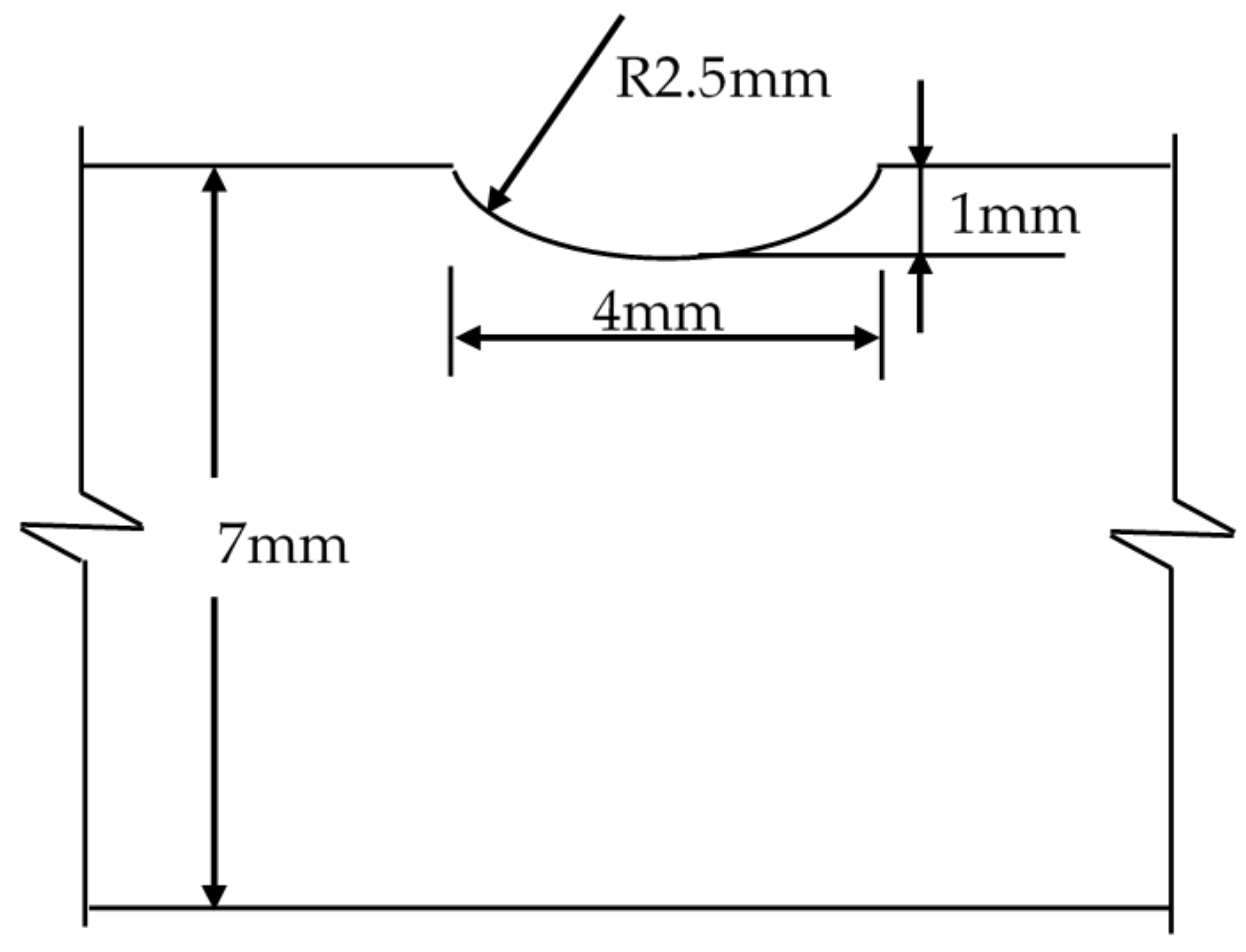
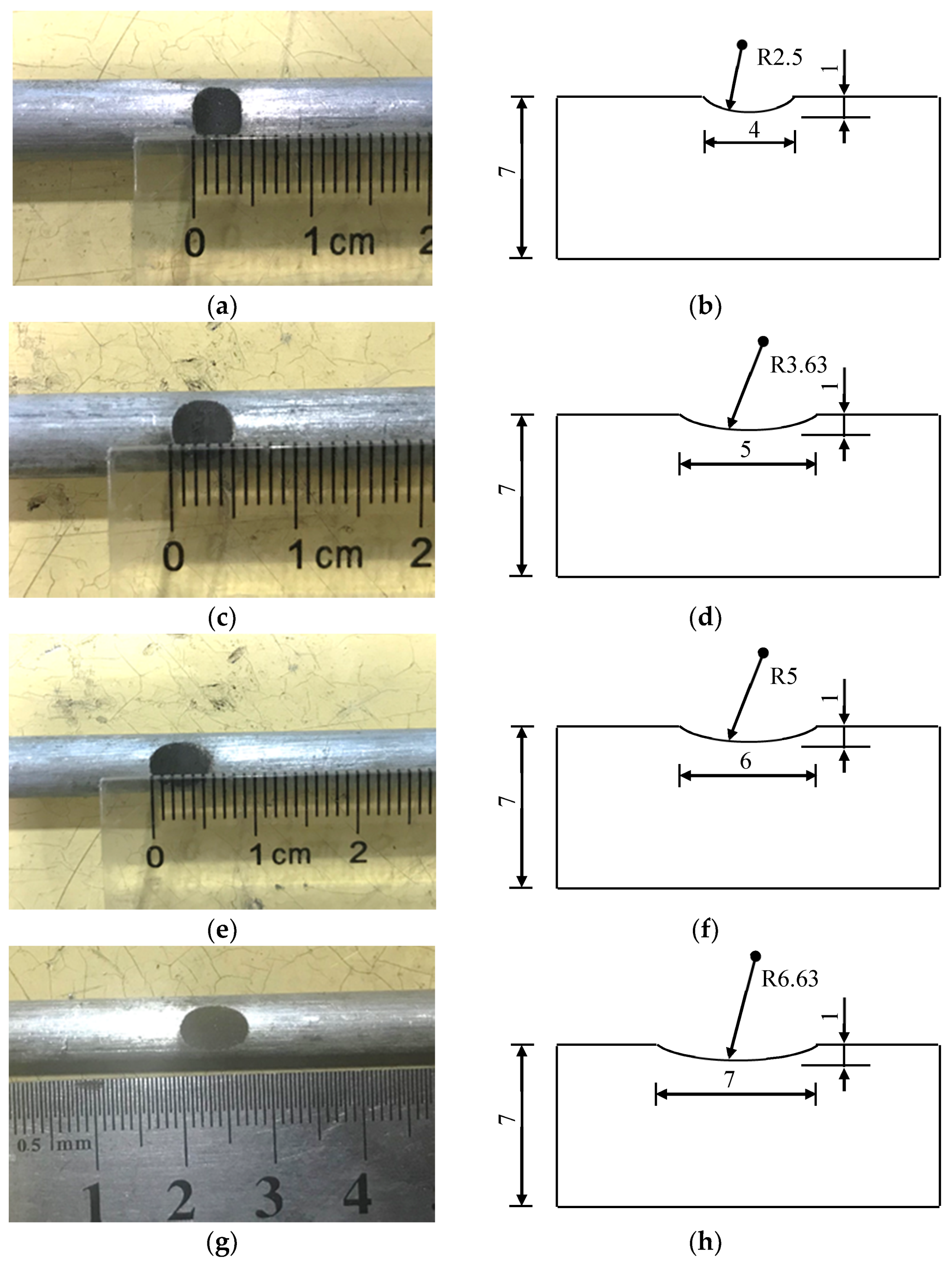
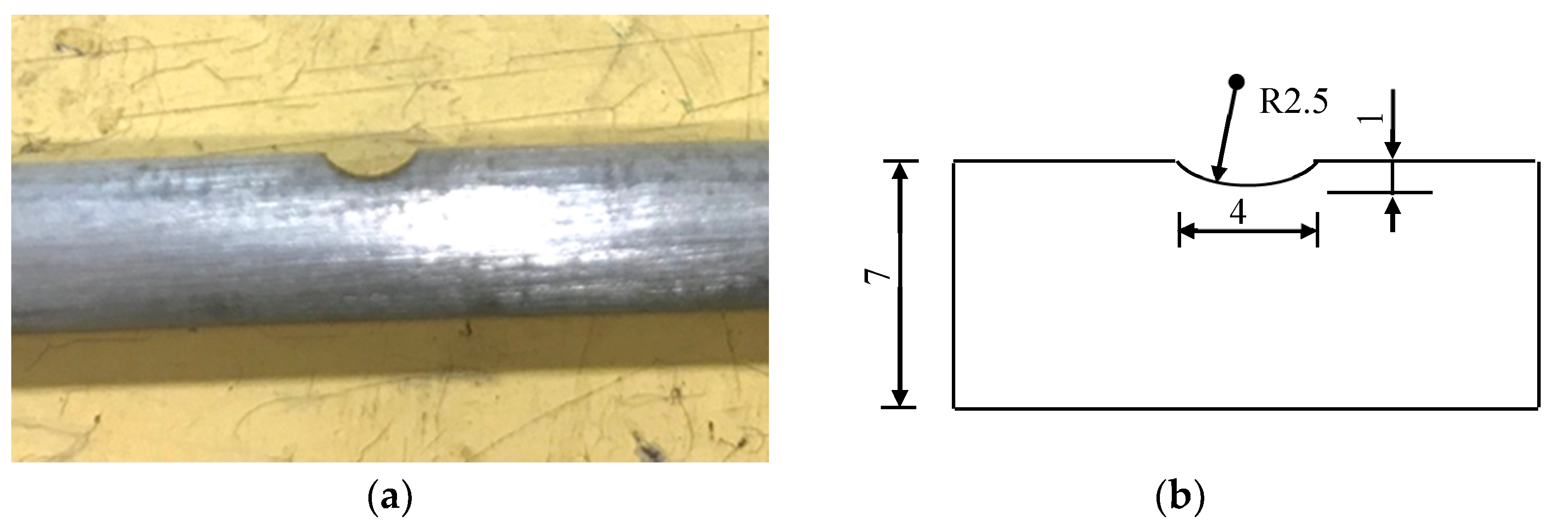
Steel wire for bridge cables in service is subjected to the fatigue loads and environmental corrosion. Corrosive medium is easy to form initial defects on the surface of steel wire. A large number of tests show that the initial defects on the surface of the old bridge cable wire caused by chlorine salt are mostly semi-ellipsoidal pits [22,23], which involves a complex electrochemical reaction process. In order to simplify the forming process of pits on steel wire surface, in this paper machine-cut notches are used to replace the pits caused by electrochemical inhomogeneity, and the effects of different notches size and morphology on fatigue crack propagation law were studied. A standard high-strength steel wire specimen with a diameter of 7 mm and a tensile strength of 1670 MPa specified in Chinese specification-GB/T 17,101 [24] was selected as the test specimen used in this paper, and the length of steel wire was taken to be 1100 mm. The steel grade of high-strength steel wire is S82B, and its chemical composition is shown in Table 1. Zn99.99 is the zinc used in the steel wire galvanized layer, and its chemical composition is shown in Table 2. The fabrication technology processing of steel wire includes pickling, phosphating, drawing, cleaning, hot-dip galvanizing, and stabilization, among which the stabilization process involves the heat treatment process. Domestic Stelmor air-cooled wire rod is used for bridge cables. The hot rolling temperature of austenitization is 950–850 °C, and the quenching temperature of the air-cooled wire used is 620–680 °C. As the heat capacity of air is low, and the thermal stability is weak, the transformation rate of pearlite is not stable during quenching. GB/T 17,101 is the specification of hot-dip galvanized steel wire for bridge cables in China, and all information about the chemical composition and fabrication technology processing of steel wire is contained in Section 7.1 of this specification. This specification is generally in line with the requirements of BS ISO 19203:2018, and a description of the steel grade and chemical composition can be obtained from Section 7 of BS ISO 19203:2018. The schematic diagram of defects on the surface of steel wire is shown in Figure 1, and the photo of the steel wire specimen is shown in Figure 2.

Table 1.
Chemical composition of S82B.
Table 2.
Chemical composition of Zn99.99.
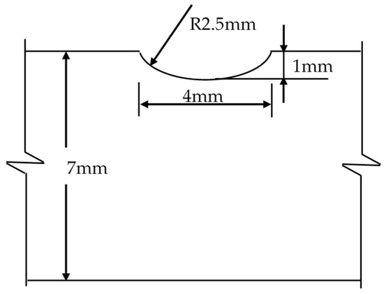
Figure 1.
Schematic diagram of machine-cut notch.
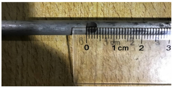
Figure 2.
Photo of steel wire specimen with machine-cut notch.
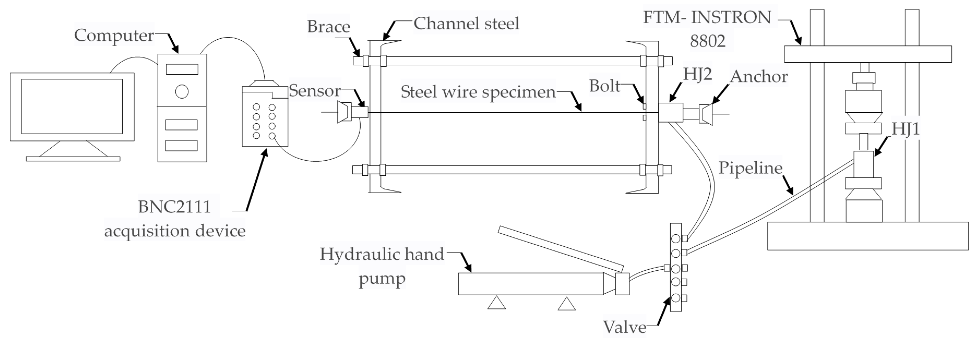
In the traditional fatigue test, the fatigue test machine (FTM) is directly used to apply the fatigue load to one specimen at a time. When the number of test specimens is large, the test will take a lot of time. In addition, due to the size limitation between the two clamps of the FTM and the vertical placement of the specimen, the corrosive medium is not easy to act on the steel wire, so the corrosion fatigue test is difficult to be realized. In view of the above reasons, a new test device is designed in this paper. The schematic diagram of the device is shown in Figure 3, consisting of two main parts. One is composed of the FTM and the hydraulic jack with large range, HJ1 for short, which are responsible for providing the total fatigue loads. HJ1 is placed between two clamps of FTM, and the oil amount of HJ1 is provided by hydraulic hand pump with oil storage capacity of 2700cc. The FTM adopted in this test is INSTRON 8802, which is shown in Figure 4. The other part is the fatigue loading device for wire specimens, as shown in Figure 5, including 40#C channel steel, braces with diameter of 20 mm, bolts, multiple hydraulic jacks with small range, HJ2s for short, anchors. HJ1 drives a series of HJ2s through tubing and diverter valve to apply fatigue loads to multiple steel wires. Data acquisition is carried out through data acquisition equipment—National Instruments BNC-2111, hollow shaft type annular force sensor and computer.
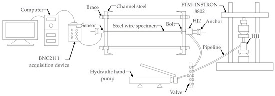
Figure 3.
Schematic diagram of loading device.
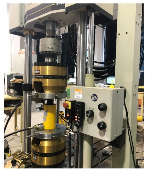
Figure 4.
Fatigue testing machine—INSTRON 8802.
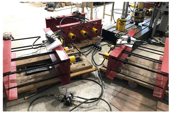
Figure 5.
Diagram of synchronous pulsation fatigue loading device.
The total oil pressure in the oil circuit can be obtained by dividing the fatigue loads applied to HJ1 by the cross section area of HJ1. This oil pressure is equally distributed to each HJ2 through the diverter valve, and the fatigue load applied to each HJ2 is equal to this oil pressure multiplied by the cross section area of the HJ2, which is also the fatigue load applied to the wire specimen connected to this HJ2. For example, the fatigue load amplitude of HJ1 applied by the FTM is 500 kN, and the cross-sectional area of HJ1 is 500 mm2, then the oil pressure amplitude is 100 MPa. This oil is equal assigned to each HJ2. If the sectional areas of three HJ2s are 100 mm2, 200 mm2 and 300 mm2 respectively, the fatigue loads of each steel wire connected to each HJ2 are 10 kN, 20 kN and 30 kN, respectively. If the diameters of the wires connected with the three HJ2s is taken as 5 mm, 6 mm, 7 mm respectively, the stress amplitude of the wire can be obtained by dividing the three load amplitudes, namely 20 kN, 40 kN and 60 kN by the cross section area of the wire, that is 509 MPa, 707 MPa and 813 MPa, respectively.
In order to investigate the influence of the combined action of the corrosive medium and fatigue loads on the crack propagation law, gauze or cotton is used to wrap the middle of notched wire specimen, and the corrosive solution is then dropped on the surface of gauze or cotton, and rapidly diffuses in the gauze or cotton to ensure full contact with the wire. Gauze or cotton not only can absorb the corrosive solution and then act on the steel wire, but also can ensure the entry of a certain amount of oxygen and reduce the volatility of the corrosive solution. It is an effective method for corrosion fatigue test. Through preliminary experiments, it was found that one hour after each drop, the surface humidity of the gauze began to change significantly an hour, and the moisture in the gauze nearly evaporated after about eight hours. Therefore, in order to ensure that the concentration of corrosive solution on the surface of the steel wire is constant, dropping is carried out every 10 min in the test. This interval is the same for all samples. The corrosion solution is selected as NaCl solution with PH of 7 and concentration of 3.5 wt%.
First, start the FTM and adjust the height of the clamp to determine the position of HJ1. Then open Valve 1 of the diverter valve and pump oil into the tubing. When filled, close Valve 1. In this way an oil circuit is formed between HJ1 and HJ2 so that the fatigue load applied to HJ1 can be transferred to HJ2 through the tubing and the diverter valve. Finally, the fatigue load amplitude, frequency and other parameters of the FTM are set, and the fatigue load applied to the HJ1 is realized by the reciprocating movement of the piston. The oil pressure applied to HJ1 is equal to the fatigue load provided by the FTM divided by the cross-sectional area of oil cylinder of the HJ1. The oil pressure of the HJ1 is transmitted to each HJ2 through each oil channel, so the force exerted on each HJ2 is equal to the oil pressure multiplied by the cross-sectional area of oil cylinder of the HJ2. This force is divided by the cross-sectional area of the steel wire to obtain the fatigue stress on the wire.
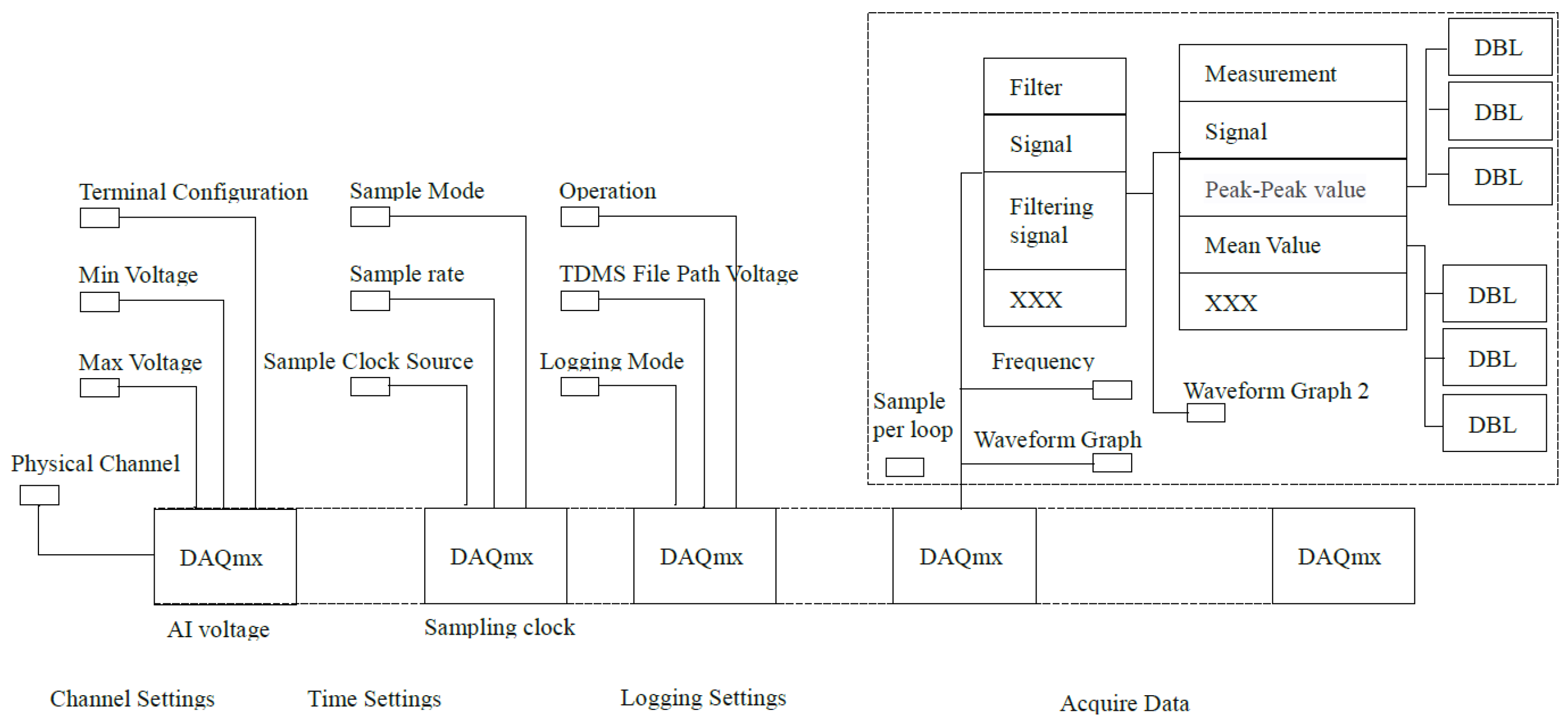
When the hydraulic system is working, the internal particles of the hydraulic oil collide with each other and produce violent friction. Hydraulic oil is also subject to friction resistance when passing through local obstacles. These will cause the loss of oil in the oil circuit and the reduction of oil pressure, ultimately consuming the energy of the whole system. Because of the resistance in the oil circuit, there is an error between the load acting on steel wire and that provided by FTM. A force sensor is used to monitor the actual load acting on steel wire and adjust it to the value set by FTM. Considering that the wire is circular, a hollow shaft type annular force sensor is selected to monitor the fatigue loads, as shown in Figure 6. The working principle of this sensor is to convert the force received by the steel wire into voltage signal. A data acquisition device, named National Instruments BNC-2111, is used to collect the voltage signal output from the sensor as shown in Figure 7. The force sensor is connected to the BNC-2111 by transmission data line. The BNC-2111 is connected to the computer. The computer can record and read the tension in each wire during fatigue loading. The Laborary Virtual Instrument Engineering Workbench (LabVIEW) software is used to calibrate the collected signal, so as to realize the conversion of voltage signal to force signal and perform the monitoring and recording of fatigue load. Figure 8 demonstrates the process and working principle of data collection by LabVIEW software, through which force loads acting on each steel wire can be collected synchronously. LabVIEW uses the graphical editing language G to write the program in block diagram form. Figure 9 shows the fatigue loads recorded by LabVIEW software, that is, the real-time forces applied to multiple steel wires and one of the wires respectively.
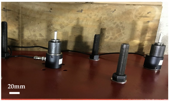
Figure 6.
Hollow shaft type annular force sensor.

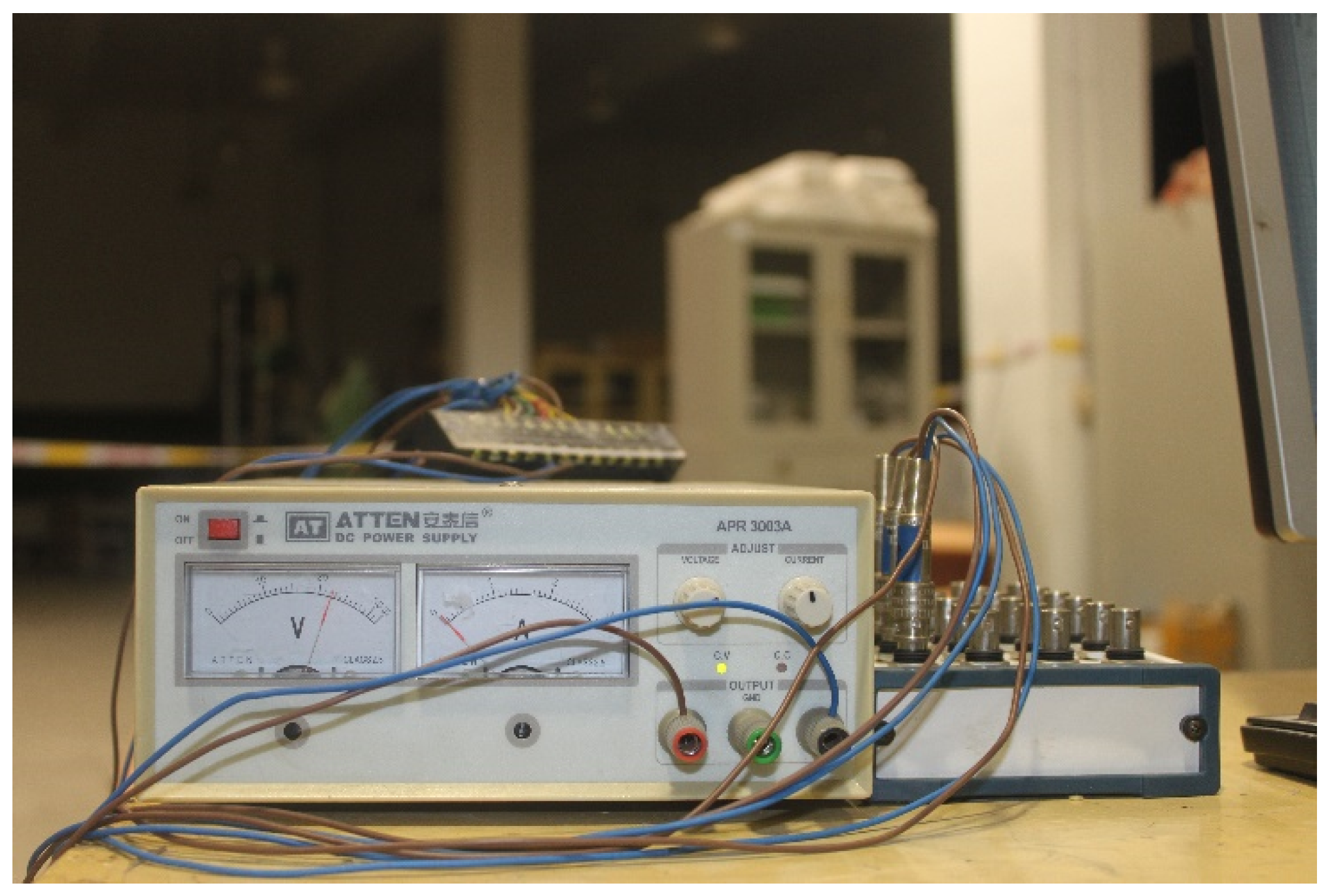
Figure 7.
Acquisition device—National Instruments BNC-2111.
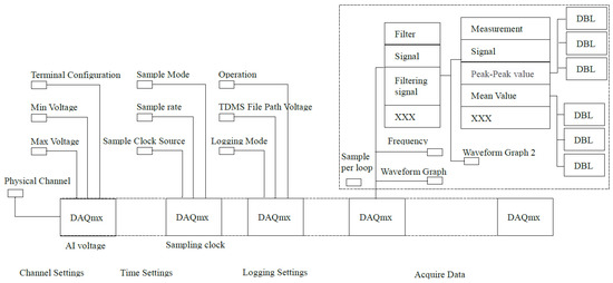
Figure 8.
Process and work principle of data collection by LabVIEW.
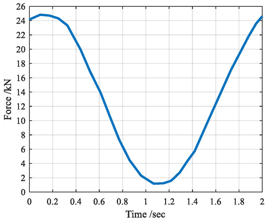
Figure 9.
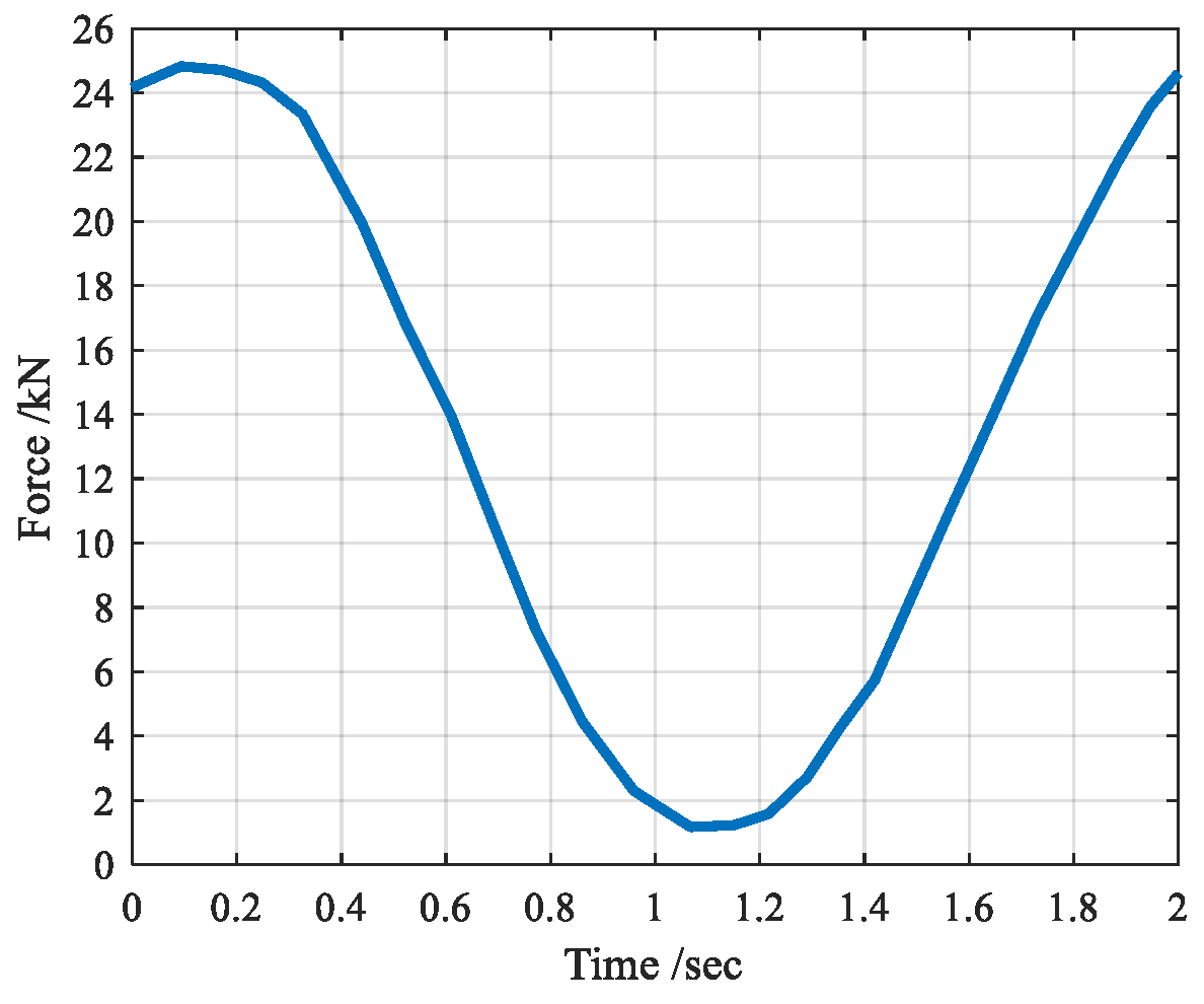
Fatigue load applied to one wire recorded by LabVIEW.
When crack propagation occurs, the plastic zone near crack tip increases, and the deformation of steel wire under maximum fatigue load increases compared with that without crack propagation, resulting in the change of the peak of loading waveform. After many tests, it is found that the peak of the loading waveform will change from single peak to short platform when the crack expands.
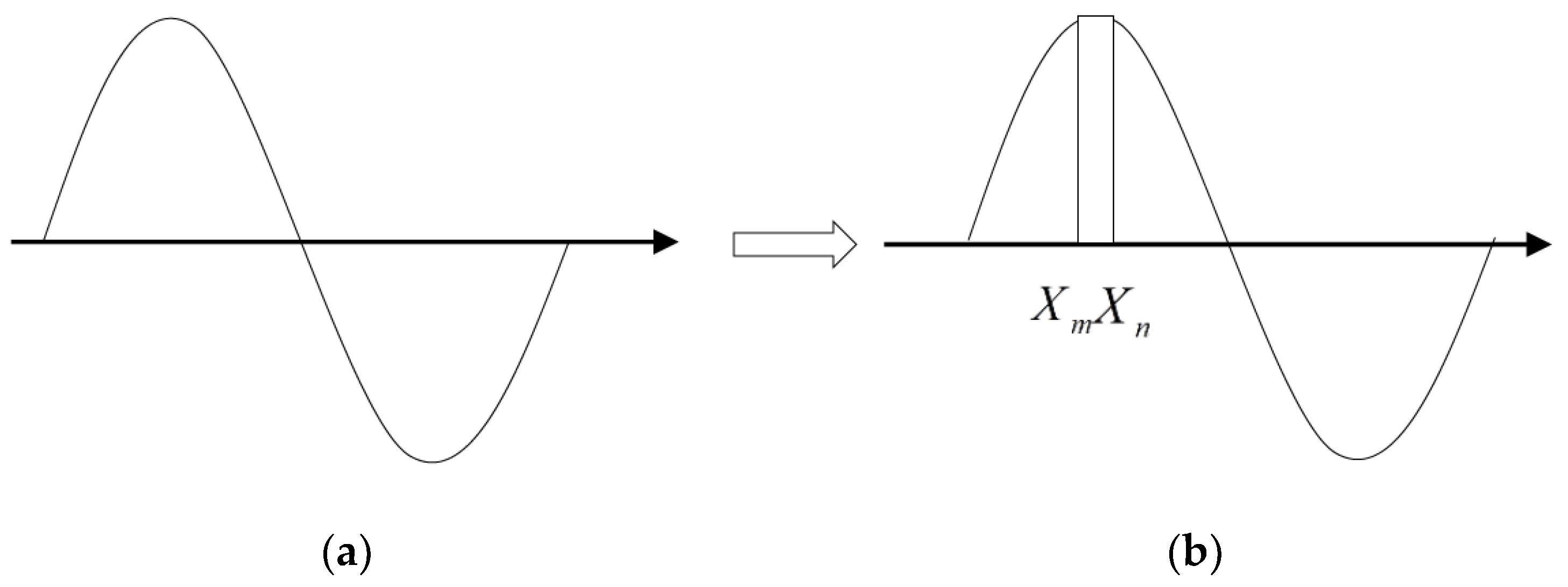
During the loading process, pay attention to the fatigue load waveform and the change of crest in the user interface of LabVIEW, as shown in Figure 10. When the crest changes from a single peak to a short platform, the change of the crest can be measured by the software measurement tool, the values of and are recorded, and the values of are defined. When it changes, the fatigue load is downloaded and the loading numbers are recorded.
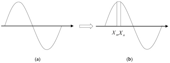
Figure 10.
The fatigue load waveform recorded by LabVIEW. (a) Waveform without crack propagation; (b) waveform with crack propagation.
After the load drops, the peak of the fatigue loading waveform is restored to a single peak. Under the action of the new fatigue load, when the crack grows again, the peak will have the same change as before, that is, from a single peak to a short platform. Similarly, the loading numbers will be recorded and the load will be lifted.
This is repeated until the steel wire breaks. The change of the crest after each load drop or load rise means that the fatigue crack has been expanded. The fatigue crack propagation process was analyzed by the recorded loading numbers and the “beach-like pattern” left by the steel wire section.
The test was conducted at room temperature, and the loading waveform was sinusoidal wave. Here, σmax is defined as the maximum stress, σmin is the minimum stress, σa is the stress range, which can be expressed as σa = σmax − σmin, R is the stress ratio, which can be expressed as R = σmin/σmax, f is the loading frequency. The parameters of the original fatigue load are set as follows: σmax = 643 MPa, σmin = 283 MPa, σa = 360 MPa, f = 0.5 Hz, R = 0.44. The parameters of the fatigue loads after downloading are set as follows: σmax = 322 MPa, σmin = 142 MPa, σa = 180 MPa, f = 0.5 Hz. R = 0.44.
3. Analysis of Macroscopic and Microcosmic Morphologies of Fatigue Fracture of Notched Wire
The analysis of fatigue fracture morphology is an important method to study the fatigue process and analyze the reasons of fatigue failure. The corrosion fatigue damage of high-strength steel wire is similar to the fracture mode of other metal materials. The fracture retains the traces of the whole fracture process and records many information occurred during the fracture process, which has obvious morphological characteristics. Therefore, macroscopic and microcosmic analysis of fatigue fracture of steel wire can accurately predict its fatigue fracture mechanism and understand its fatigue crack propagation.
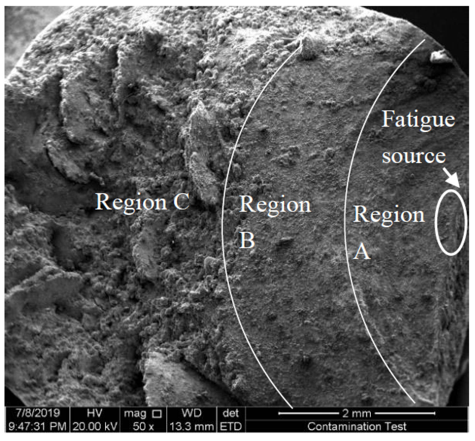
Figure 11 shows the macroscopic morphology of typical corrosion fatigue fracture of high-strength steel wire used in bridge cables. It can be seen that fatigue cracks generally start at a certain surface defect or stress concentration and slowly extend into the steel wire in a semi-circular until the steel wire suddenly breaks. The whole fatigue fracture surface can be roughly divided into three regions: slow extending region (Region A), fast extending region (Region B) and instantaneous fracture region (Region C). From Figure 11, it can be seen that slow extending region is relatively smooth, fatigue cracks extend inward in circular arc. This is mainly because the stress intensity factor (SIF) at the crack tip is relatively small at the initial crack propagation stage. Each time the steel wire undergoes a cyclic load, the crack tip advances a tiny distance, so the law of crack propagation at this stage is relatively stable. Thus, this stage is commonly referred to as the steady-state extension stage. With the continuous application of cyclic load, the stress intensity factor at the crack tip increases as the crack grows into the material, and the crack propagation rate changes from slow to fast, so the cracks enter the fast extending region. At this stage, the crack propagation depth under each cyclic load is greater than that in the steady-state region, which is the transition region between the steady-state region and the instantaneous fracture region. When the cracks grow to a certain depth, the effective cross-sectional area of the steel wire will be reduced to a critical value. At this time, the fracture toughness cannot resist the stress intensity at the crack tip, so the cracks enter the unsteady-state extension stage, and the steel wire breaks instantly. As can be seen from the macroscopic morphology of the steel wire fracture surface, the instantaneous fracture region is relatively rough with obvious radial fibers.
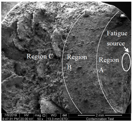
Figure 11.
Macroscopic morphology of fatigue crack propagation.
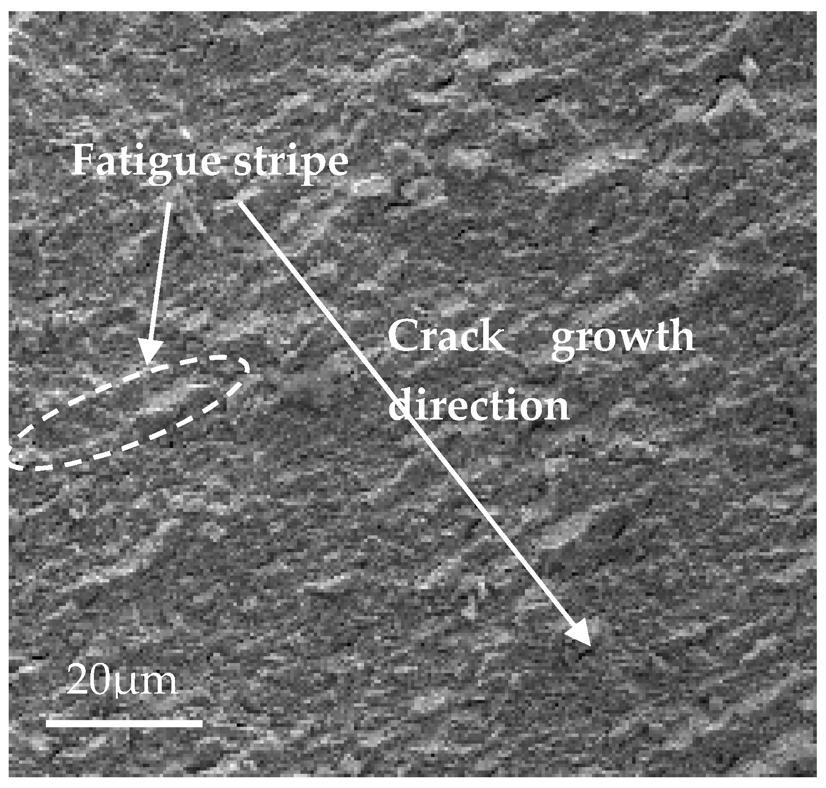
Figure 12 show the microcosmic morphology of the fatigue fracture of steel wire with slow extending region. Under the continuous application of cyclic load, cracks begin to form at a certain defect position or stress concentration point of the steel wire, which become the origin points of fatigue cracks. As the load increases, the cracks extend into the material. When the cracks are in the slow extending region, the speed of extension is relatively slow, and the fatigue stripes can be seen, which is perpendicular to the crack propagation direction, as shown in Figure 12. The crack propagation of the steel wire in the slow extending region is transgranular fracture, as shown in Figure 13. When the cracks enter the fast extending region, the speed of fatigue crack propagation is relatively fast and transgranular fracture (same as the slow extending region). The crack propagation morphology showed circular arcs along the crack propagation direction. The microcosmic morphology of this stage shows that the cross section is relatively rough. As the fatigue cracks extend further, the bearing capacity of the specimen continues to decrease. Because the area of the effective bearing surface decreases constantly, the stress of the crack front increases. When the stress reaches the critical fracture strength, the specimen will be fractured in an instant. The fracture morphology of the instantaneous fracture region is similar to that of the static load tensile specimen, both of which are typical dimple features, as shown in Figure 14.
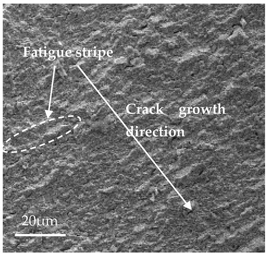
Figure 12.
Mesoscopic morphology of Region A—slow extending region.
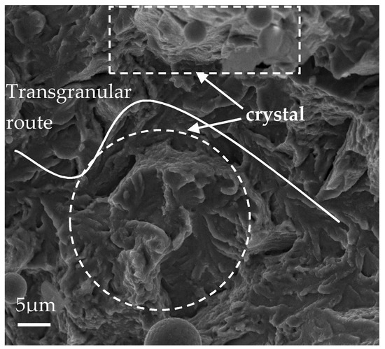
Figure 13.
Mesoscopic morphology of transgranular fracture.
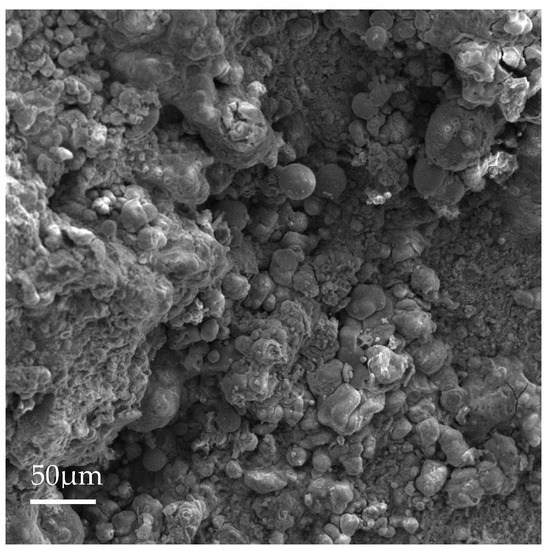
Figure 14.
Mesoscopic morphology of Region C—instantaneous fracture region.
4. Analysis of Fatigue Crack Propagation Test Results
4.1. Effect of Semi-Ellipsoidal Notch Depth on Crack Propagation Rate
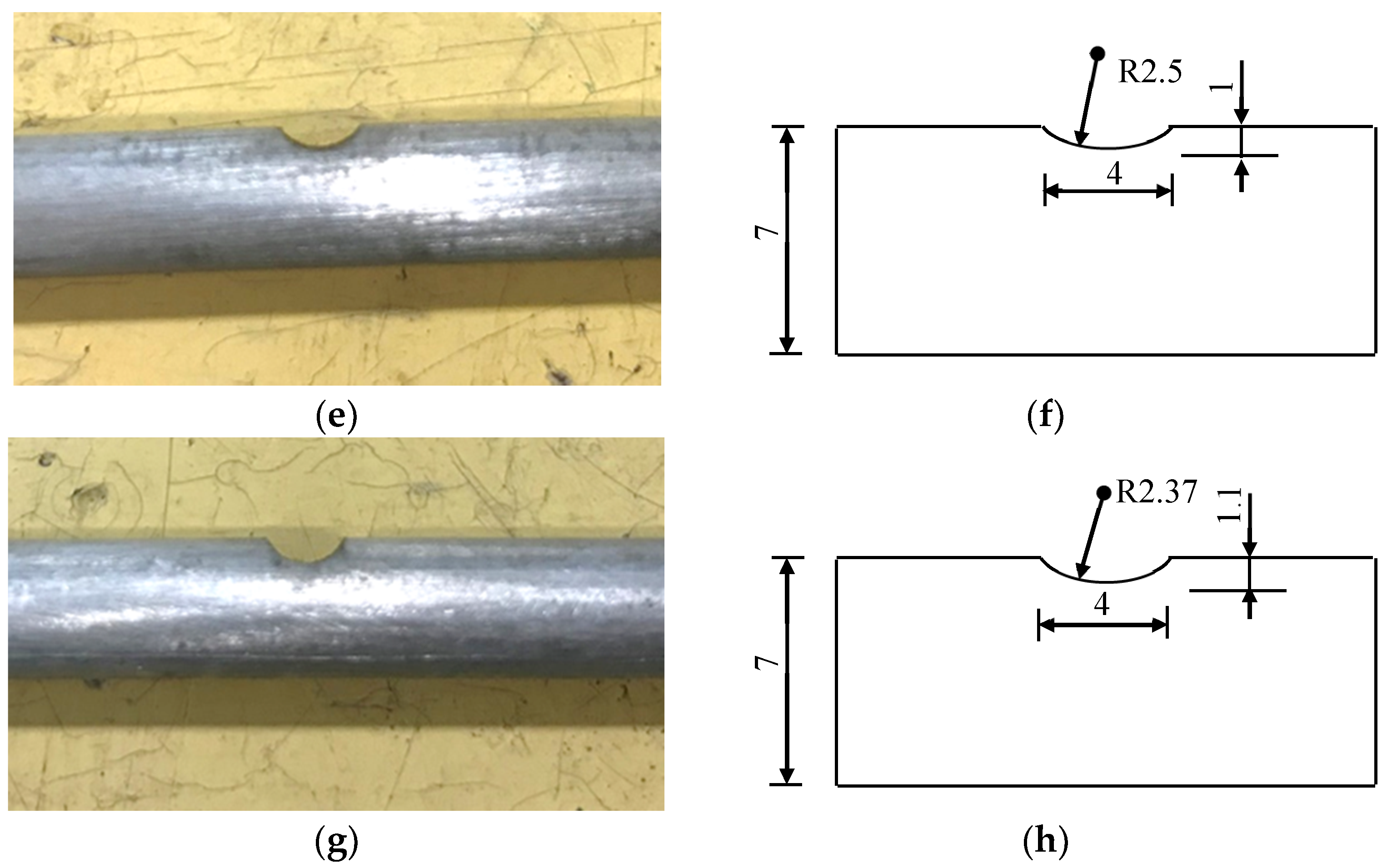
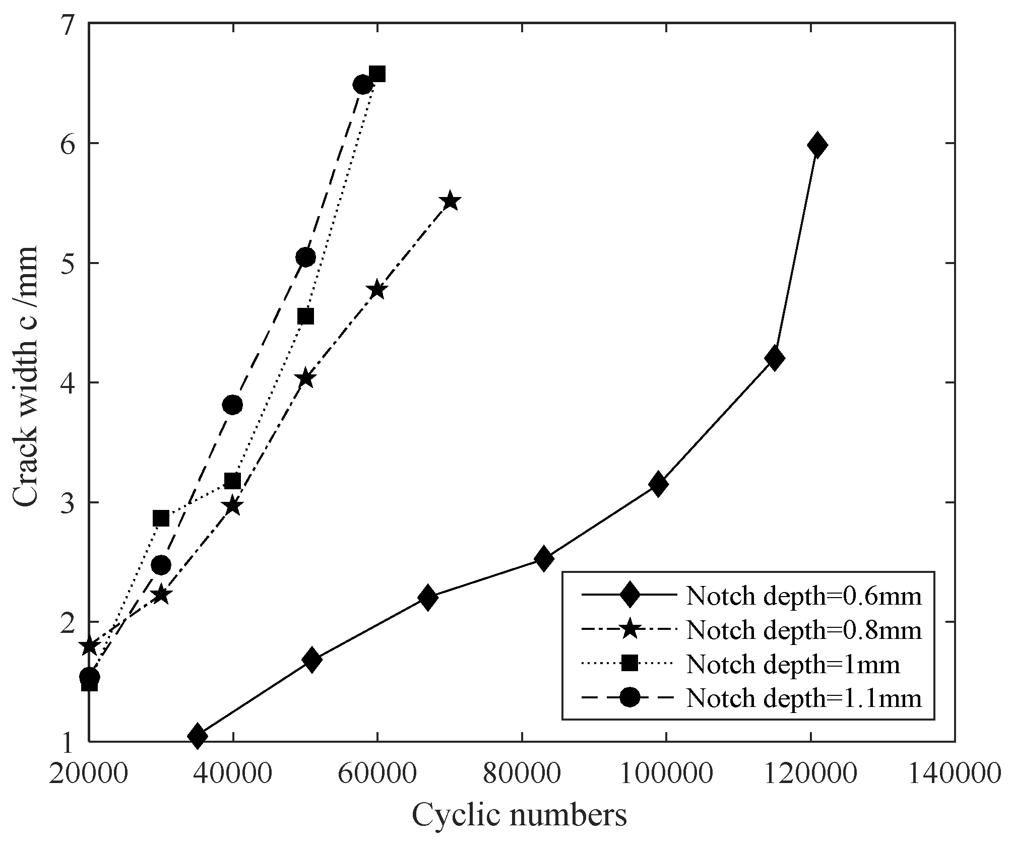
In order to investigate the influence of depth of machine-cut notches on the fatigue crack propagation of steel wire, semi-ellipsoidal notches with different depths are used for the test in this paper. The depths are taken as 0.6 mm, 0.8 mm, 1.0 mm and 1.1 mm, respectively. The widths of semi-ellipsoidal notches are all 4 mm. The schematic diagram of steel wire and corresponding wire specimen with semi-ellipsoidal notches of different depths are shown in Figure 15.
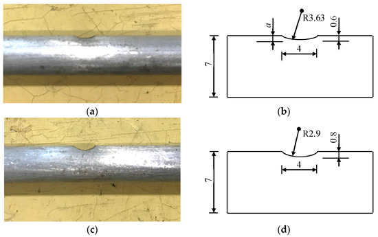
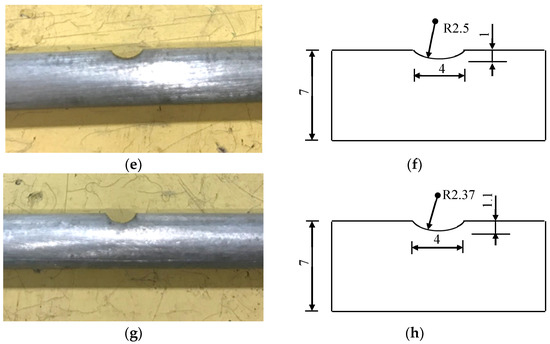
Figure 15.
Wire specimens with different semi-ellipsoidal notches of different depths. (a) No. D-1 Steel wire specimen; (b) dimension of No. D-1 steel wire; (c) No. D-2 steel wire specimen; (d) dimension of No. D-2 steel wire; (e) No. D-3 steel wire specimen; (f) dimension of No. D-3 steel wire; (g) No. D-4 steel wire specimen; and (h) dimension of No. D-4 steel wire.
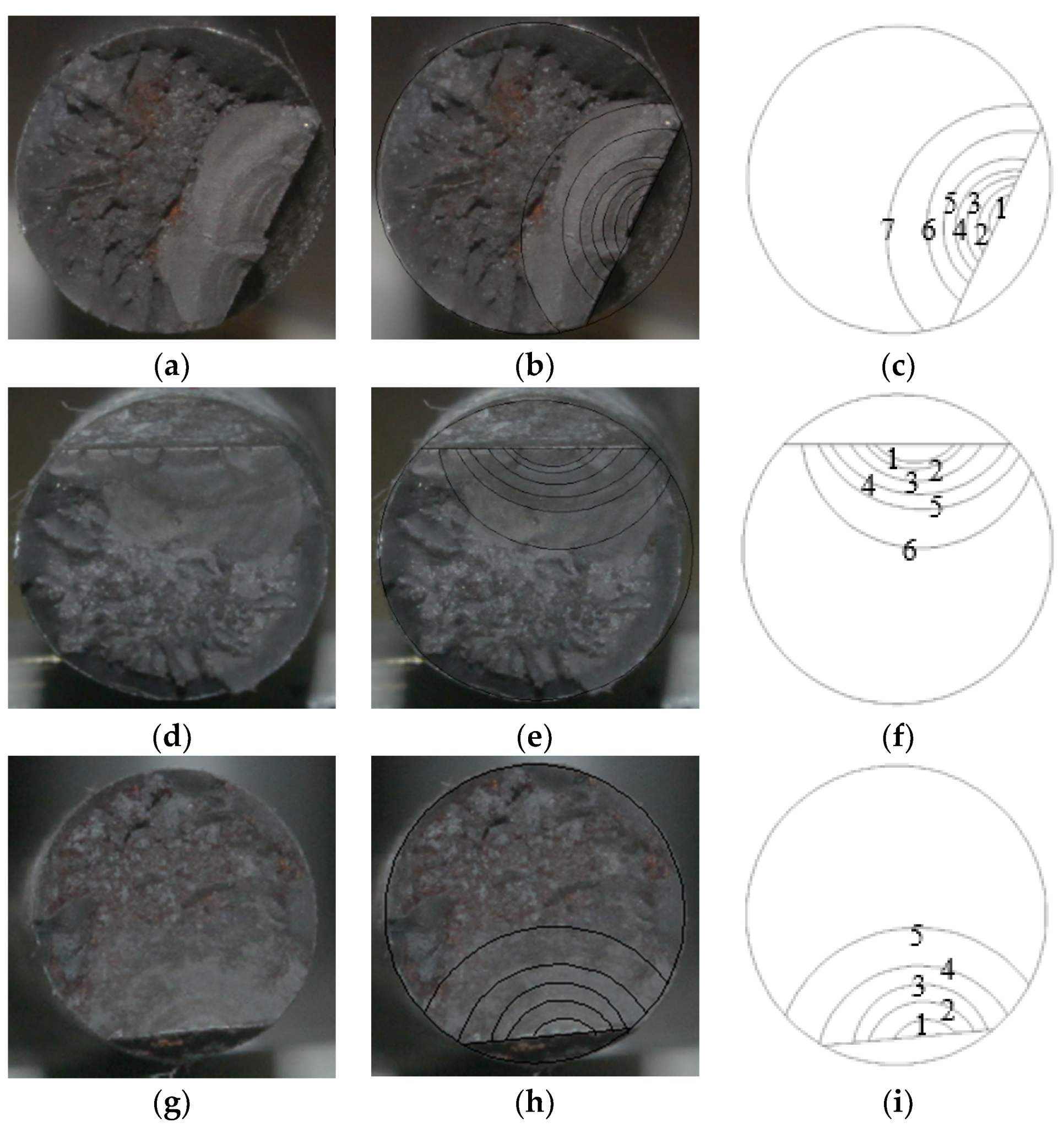
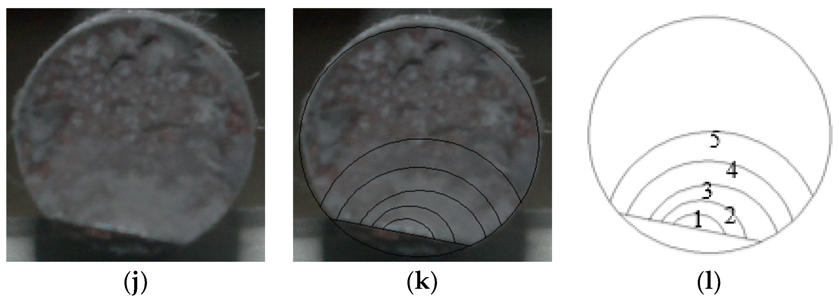
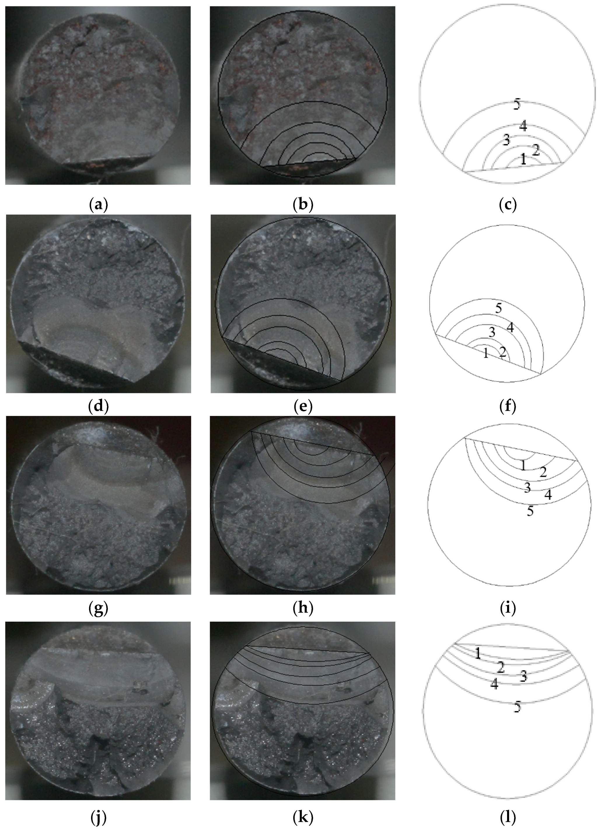
Figure 16 shows the section morphologies of the four specimens without the hooking, the section morphologies with the hooking and the schematic diagrams of the hooking. It can be seen that with the increase of loading numbers, the four specimens all have different beach-like load shedding lines at the cross section.
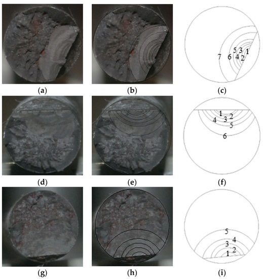
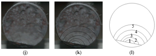
Figure 16.
Steel wire sections with notches at different depths. (a) D-1 without “bench-like pattern” hooking; (b) D-1 with “bench-like pattern”; (c) schematic diagram of D-1 wire specimen; (d) D-2 without “bench-like pattern”; (e) D-2 with“bench-like pattern”; (f) schematic diagram of D-2 wire specimen; (g) D-3 without“bench-like pattern”; (h) D-3 with “bench-like pattern”; (i) schematic diagram of D-3 wire specimen; (j) D-4 without “bench-like pattern”; (k) D-4 with “bench-like pattern”; (l) schematic diagram of D-4 wire specimen.
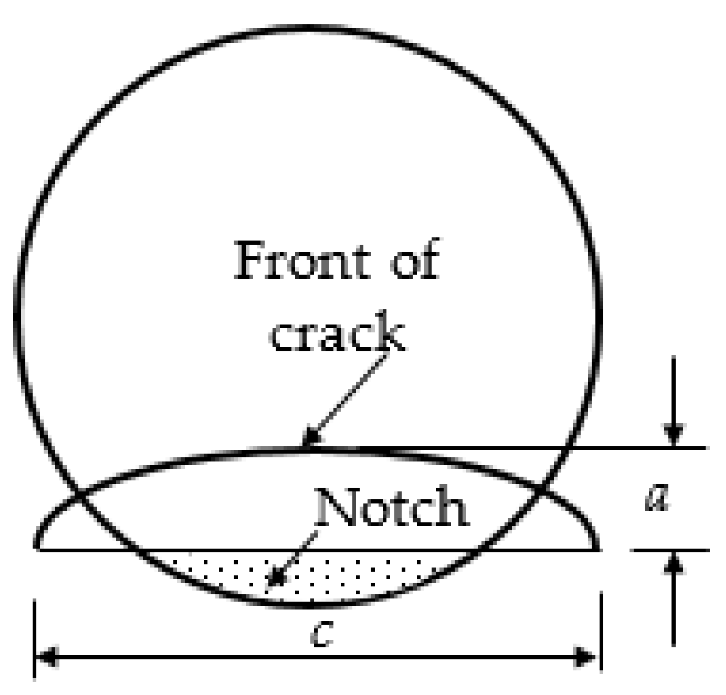
Figure 17 shows the schematic diagram of crack depth and width, a is the depth of the crack, which is the length of the beach-like pattern camber from the surface of the prefabricated notch. c is the width of the crack, which is the distance between two points where the beach-like pattern intersects the straight line of the prefabricated notch section.
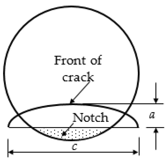
Figure 17.
Schematic diagram of crack depth a and width c.
Table 3 shows the change of the crack depth and width of the four groups of steel wires with the loading numbers. a is the crack depth, c is the crack width, and N is the cyclic loading numbers.
Table 3.
Test data of steel wire crack propagation with notches of different depths.
Figure 18 and Figure 19 show the change of crack depth and width with fatigue loading numbers obtained according to the data in Table 1. It can be seen that the crack propagation rate is slow at first, but gradually accelerates. The deeper the initial depth of the notch, the faster the rate of crack propagation.
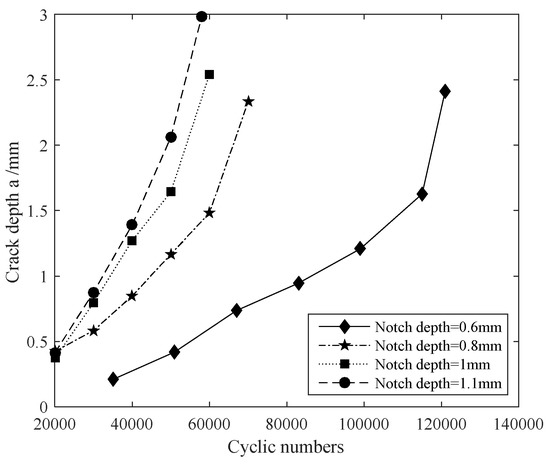
Figure 18.
Variation of crack depth with cyclic numbers.
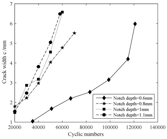
Figure 19.
Variation of crack width with cyclic numbers.
It can also be seen from Figure 18 and Figure 19 that both crack depth and crack width show a law which are similar to linear propagation with the change of fatigue loading numbers. In order to distinguish the influence of initial notch depth on crack propagation, the a-N curve and c-N curve were linear fitted, , . The specific results are shown in Table 4. It can be seen that the slope of the fitting line corresponding to the specimen with a larger notch depth is higher. That is, the deeper the notch depth is, the higher the crack propagation rate is.
Table 4.
Coefficient table.
4.2. Effect of Semi-Ellipsoidal Notch Width on Crack Propagation Rate
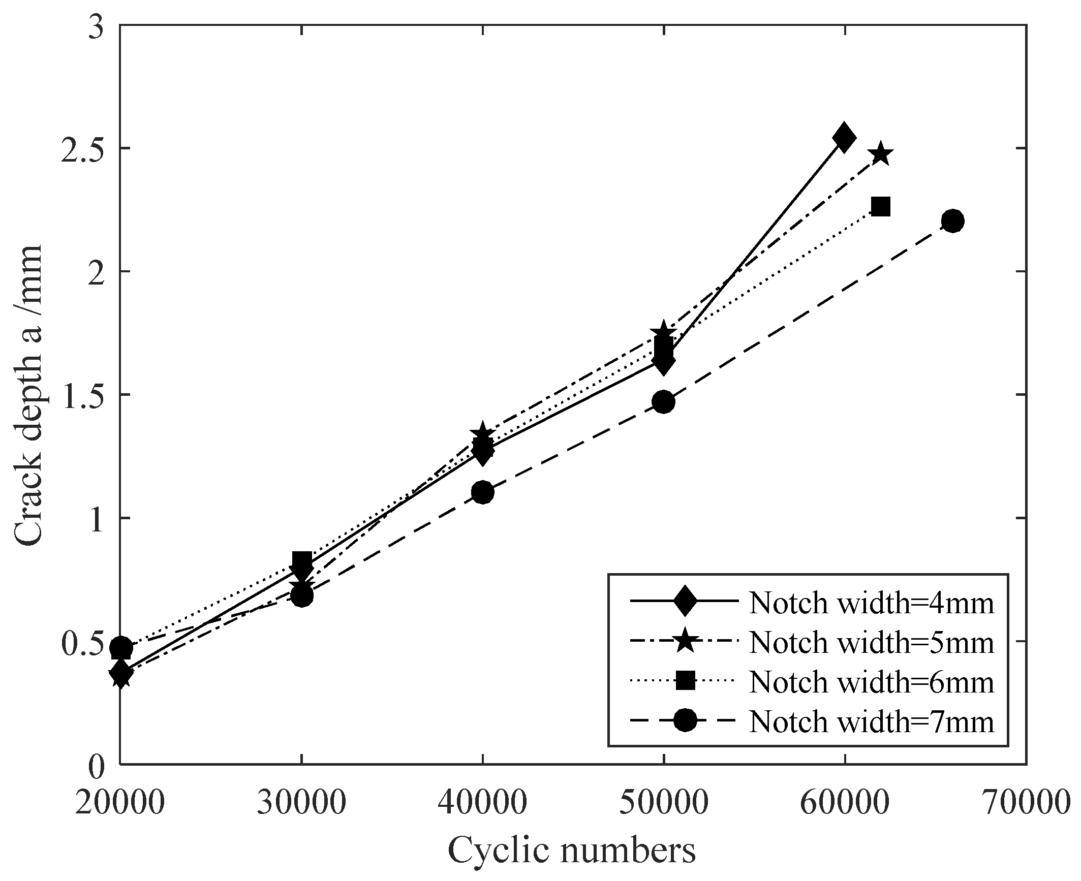
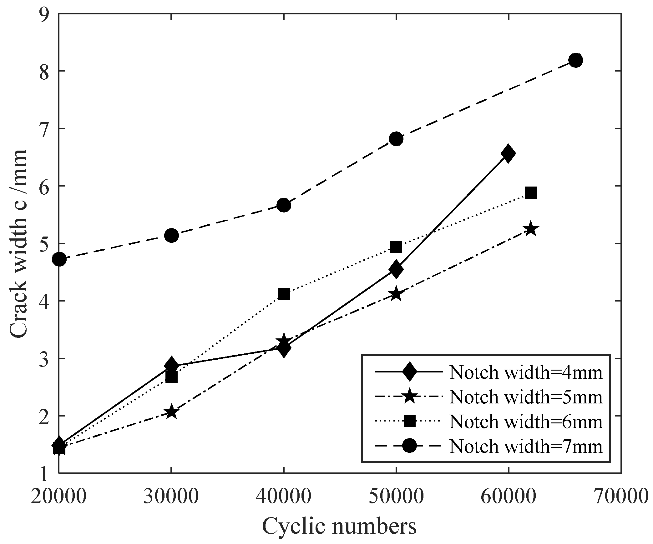
In order to investigate the influence of width of machine-cut notches on the fatigue crack propagation of steel wire, semi-ellipsoidal notches with different widths are used for the test in this paper. The widths are taken as 4 mm, 5 mm, 6 mm and 7 mm respectively. The depths of semi-ellipsoidal notches are all 1 mm. The schematic diagram of steel wire and corresponding wire specimen with semi-ellipsoidal notches of different widths are shown in Figure 20.

Figure 20.
Wire specimens with semi-ellipsoidal notches of different widths. (a) No. L-1 steel wire specimen; (b) dimension of No. L-1 steel wire; (c) No. L-2 steel wire specimen; (d) dimension of No. L-2 steel wire; (e) No. L-3 steel wire specimen; (f) dimension of No. L-3 steel wire; (g) No. L-4 steel wire specimen; and (h) dimension of No. L-4 steel wire.
Figure 21 shows the section morphologies of the four specimens without the hooking, the section morphologies with the hooking and the schematic diagrams of the hooking. It can be seen that with the increase of loading numbers, the four specimens all have different beach-like load shedding lines at the cross section.
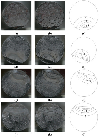
Figure 21.
Steel wire sections with notches at different widths. (a) L-1 without “bench-like pattern”; (b) L-1 with “bench-like pattern”; (c) schematic diagram of L-1 wire specimen; (d) L-2 without “bench-like pattern”; (e) L-2 with“bench-like pattern”; (f) schematic diagram of L-2 wire specimen; (g) L-3 without “bench-like pattern”; (h) L-3 with “bench-like pattern”; (i) schematic diagram of L-3 wire specimen; (j) L-4 without “bench-like pattern”; (k) L-4 with “bench-like pattern”; and (l) schematic diagram of L-4 wire specimen.
Table 5 show the change of crack depth and width of four groups of steel wires with the loading numbers during the test. In the table, a is the depth of crack, c is the width of crack, and N is cyclic loading numbers.
Table 5.
Test data of steel wire crack propagation with notches of different widths.
Figure 22 and Figure 23 show the change of crack depth and width with fatigue loading numbers obtained according to the data in Table 3. It can be seen that the rate of crack propagation presents a uniform trend. The smaller the initial width of the notch, the faster the rate of crack propagation.
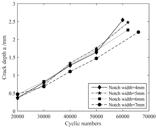
Figure 22.
Variation of crack depth with cyclic numbers.
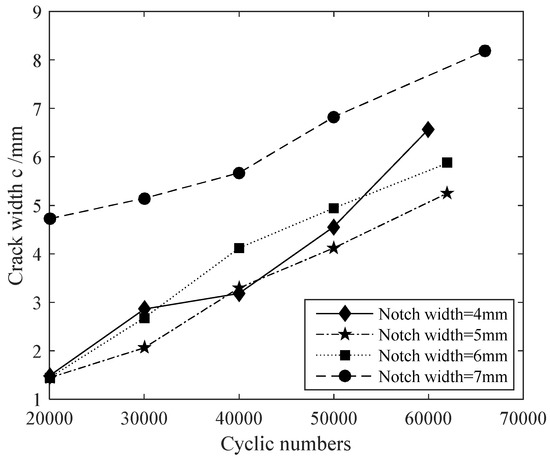
Figure 23.
Variation of crack width with cyclic numbers.
It can also be seen from Figure 22 and Figure 23 that both crack depth and crack width show a law which are similar to linear propagation with the change of fatigue loading numbers. In order to distinguish the influence of initial notch width on crack propagation, the a-N curve and c-N curve were linear fitted, , . The specific results are shown in Table 6. It can be seen that the slope of the fitting line corresponding to the specimen with a smaller notch width is higher. That is, the smaller the notch width is, the higher the crack propagation rate is.
Table 6.
Coefficient table.
4.3. Effect of Notch Shape on Crack Propagation Rate
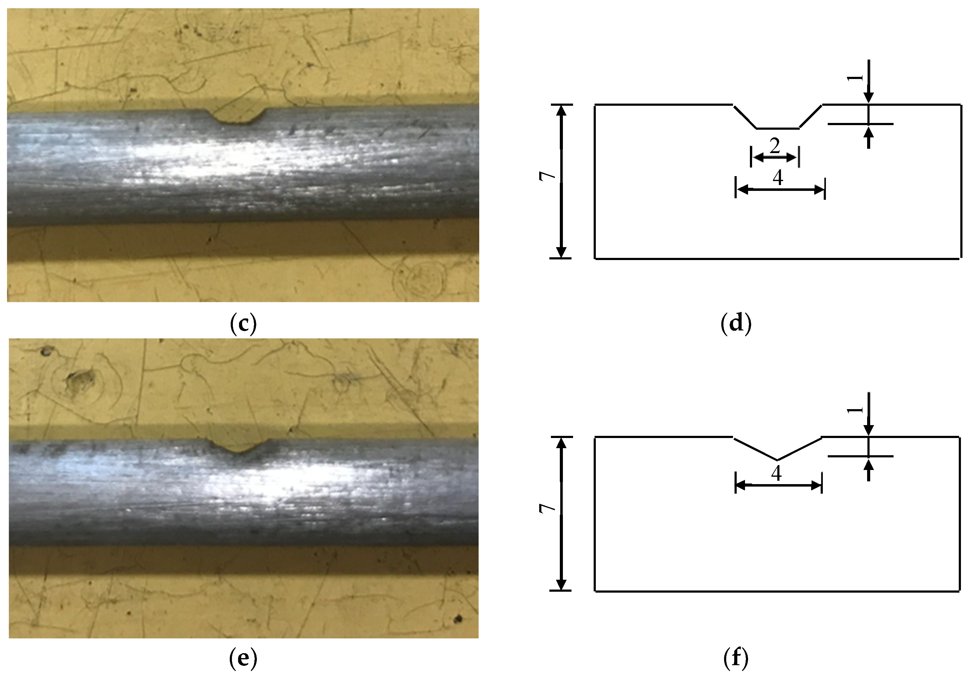
In order to investigate the influence of shape of machine-cut notches on the fatigue crack propagation of steel wire, notches with different shapes are used for the test in this paper. S-1, S-2 and S-3 represent the specimens with semi-ellipsoidal notch, trapezoidal notch and v-shaped notch, respectively. The schematic diagram of steel wire and corresponding wire specimen with notches of different shapes are shown in Figure 24.
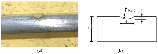
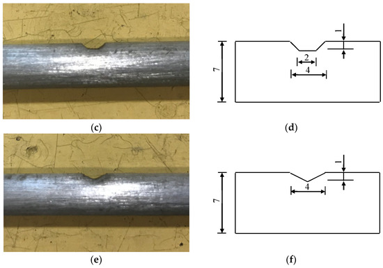
Figure 24.
Wire specimens with machine-cut notches of different shapes. (a) No. S-1 steel wire specimen; (b) dimension of No. S-1 steel wire; (c) No. S-2 steel wire specimen; (d) dimension of No. S-2 steel wire; (e) No. S-3 steel wire specimen; and (f) dimension of No. S-3 steel wire.
Figure 25 shows the section morphologies of the three specimens without the hooking, the section morphologies with the hooking and the schematic diagrams of the hooking. It can be seen that with the increase of loading numbers, the three specimens all have different beach-like load shedding lines at the cross section.
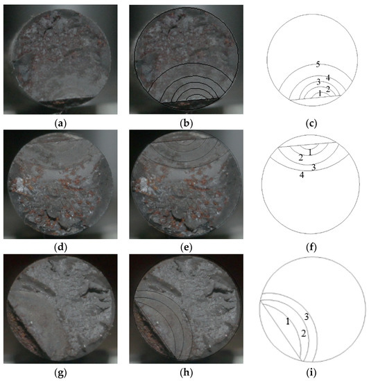
Figure 25.
Steel wire sections with notches at different shapes. (a) S-1 without “bench-like pattern”; (b) S-1 with “bench-like pattern”; (c) schematic diagram of S-1 wire specimen; (d) S-2 without “bench-like pattern”; (e) S-2 with “bench-like pattern”; (f) schematic diagram of S-2 wire specimen; (g) S-3 without “bench-like pattern”; (h) S-3 with “bench-like pattern”; and (i) schematic diagram of S-3 wire specimen.
Table 7 shows the change of crack depth and width of three groups of steel wires with the cyclic loading numbers. Here, a is the depth of crack; c is the width of crack, and N is cyclic loading numbers.
Table 7.
Test data of steel wire crack propagation with notches of different shapes.
Figure 26 shows the variation of crack depth with cyclic numbers according to the data in Table 7. It can be seen that the rate of crack propagation presents a uniform trend. The sharper the shape of the notch, the faster the rate of crack propagation.
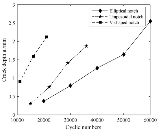
Figure 26.
Variation of crack depth with cyclic numbers.
It can also be seen from Figure 26 that the crack depth shows a linear correlation with the cyclic loading numbers. In order to distinguish the influence of notch shape on crack propagation, linear fit is used for the a-N and c-N curves. , . The fitting coefficients are shown in Table 8. It can be seen that the sharper the notch shape, the larger the coefficient A, and the higher the crack propagation rate.
Table 8.
Coefficient table.
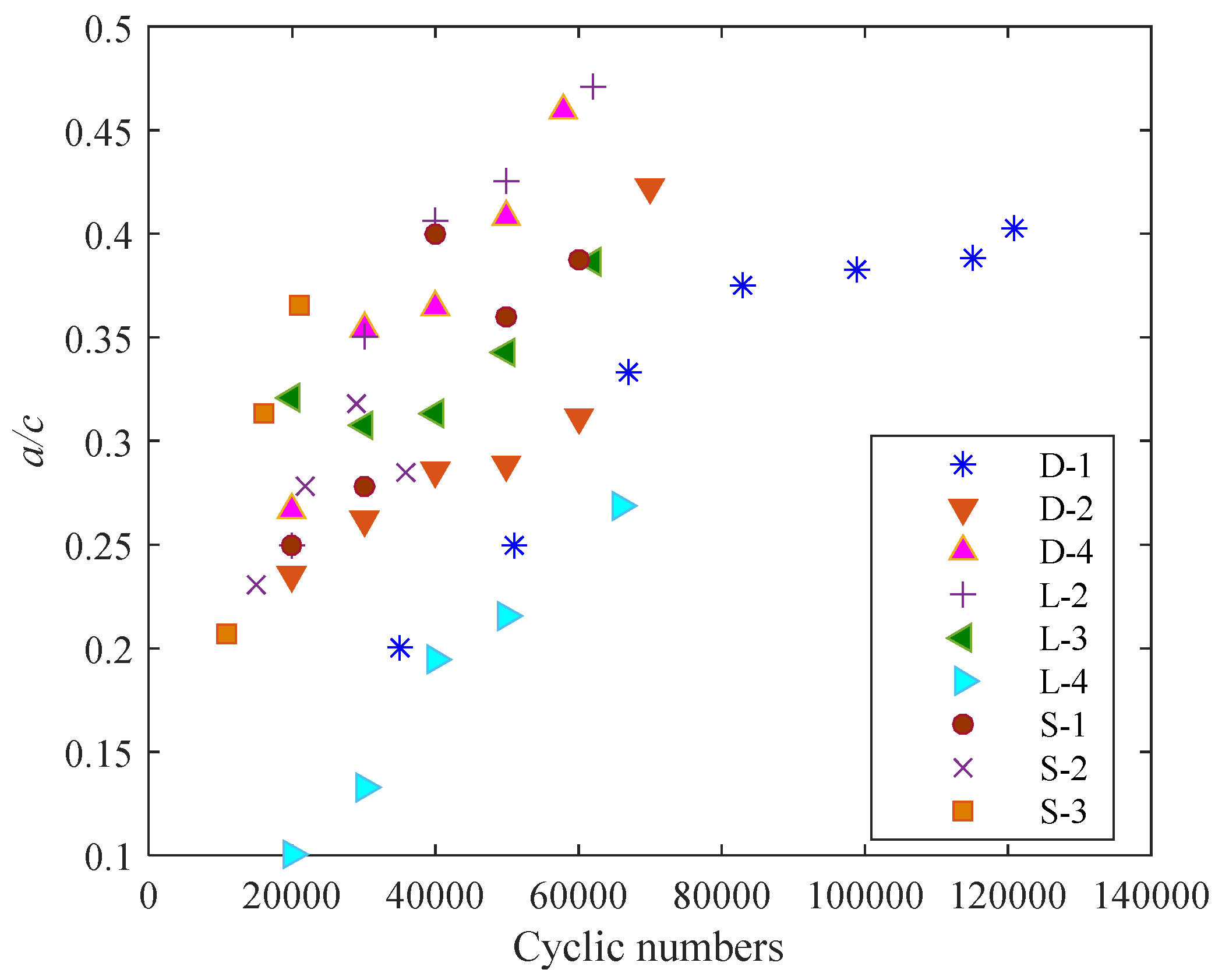
Figure 27 shows the scatter diagram of a/c varying with the cyclic loading numbers during the crack propagation of each group of steel wires. It can be seen that the ratio of a to c of each specimen is between 0.2 and 0.4, which indicates that in the case of uniaxial tension, the surface crack usually remains semi-elliptic during the propagation process. With the increase of cyclic numbers, the ratio of a to c gradually increases, which indicates that the crack propagation rate along the depth direction is higher than that along the width direction, but the shape of the crack front remains semi-elliptic during the crack propagation.
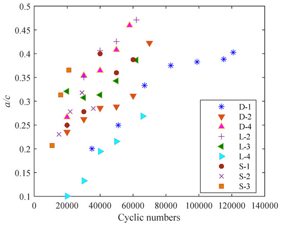
Figure 27.
Variation of a/c with cyclic numbers.
5. Conclusions
In this paper, the fatigue crack propagation tests of high-strength steel wire used in bridge cables with machine-cut notches were carried out by combining crack front marking technique and AutoCAD software. The influence of depth, width and shape of initial defects on fatigue crack propagation rate of steel wire specimen was quantitatively analyzed through the relationship between fatigue crack length and cyclic loading numbers. Major conclusions from this study can be summarized as follows:
- (1)
- The test device designed in this paper can effectively realize the synchronous pulsation fatigue loading, and simultaneously apply different fatigue stress ranges to multiple steel wires, which greatly reduces the test period.
- (2)
- The method to identify fatigue crack propagation based on load waveform variation in this paper can directly and accurately judge the moment of fatigue crack propagation, and the limitation of previous empirical method can be solved.
- (3)
- The fatigue fracture of the steel wire was analyzed macroscopically and microcosmically, and three regions of fatigue fracture were found: slow extending region (Region A), fast extending region (Region B) and instantaneous fracture region (Region C), and the behavior of fatigue crack propagation in each region was investigated.
- (4)
- The fatigue crack propagation tests of high-strength steel wire used in bridge cables with different prefabricated defects were carried out in this paper. The influence of depth, width and shape of initial defects on fatigue crack propagation rate of steel wire specimen was quantitatively analyzed through the relationship between fatigue crack length and cyclic loading numbers. The results show that the larger the depth, the smaller the width and the sharper the shape of initial defect, the faster the crack propagation rate and the lower fatigue life of steel wire.
Author Contributions
Conceptualization, Y.W.; methodology, Y.W.; writing—original draft preparation, W.Z.; writing—review and editing, X.P.; supervision, Y.Z.; project administration, Y.W.; funding acquisition, Y.W. All authors have read and agreed to the published version of the manuscript.
Funding
This research was funded by the grant from National Natural Science Foundation of China (Grant No. 51678135); Natural Science Foundation of Jiangsu Province (No. BK20171350); Six Talent Peak Projects in Jiangsu Province (JNHB-007), and the China Scholarship Council (No.201906090261), which are gratefully acknowledged.
Conflicts of Interest
The authors declare that they have no known competing financial interests or personal relationships that could have appeared to influence the work reported in this paper.
References
- Barton, S.C.; Vermaas, G.W.; Duby, P.F. Accelerated corrosion and embrittlement of High-Strength bridge wire. J. Mater. Civ. Eng. 2000, 12, 33–38. [Google Scholar] [CrossRef]
- Pan, X.; Xie, X.; Li, X. Mechanical properties and grading method of corroded high-tensile steel wires. J. Zhejiang Univ. (Eng. Sci.) 2014, 48, 1917–1924. [Google Scholar]
- Mahmoud, K.M. Fracture behavior and strength assessment of bridge cable wire. In Proceedings of the International Conference on Fatigue & Fracture in the Infrastructure: Bridges & Structures of Century, Philadelphia, PA, USA, 6–9 August 2006. [Google Scholar]
- Beretta, S.; Matteazzi, S. Short crack propagation in eutectoid steel wires. Int. J. Fatigue 1996, 18, 451–456. [Google Scholar] [CrossRef]
- Yang, F.P.; Kuang, Z.B.; Shlyannikov, V.N. Fatigue crack propagation for Straight-Fronted edge crack in a round bar. Int. J. Fatigue 2006, 28, 431–437. [Google Scholar] [CrossRef]
- Andrea, C. Shape change of surface cracks in round bars under cyclic axial loading. Int. J. Fatigue 1993, 15, 21–26. [Google Scholar]
- McFadyen, N.B.; Bell, R.; Vosikovsky, O. Fatigue crack propagation of semielliptical surface cracks. Int. J. Fatigue 1990, 12, 43–50. [Google Scholar] [CrossRef]
- Nakamura, S.-I.; Suzumura, K.; Tarui, T. Mechanical properties and remaining strength of corroded bridge wires. Struct. Eng. Int. 2004, 14, 50–54. [Google Scholar] [CrossRef]
- Miyachi, K.; Nakamura, S. Experimental and analytical study on fatigue strength and stress concentration of corroded bridge wires. Bridge Struct. 2016, 12, 21–31. [Google Scholar] [CrossRef]
- Li, X.Z.; Xie, X.; Pan, X.Y. Experimental study on fatigue performance of corroded high tensile steel wires of arch bridge hangers. China Civ. Eng. J. 2015, 48, 68–76. [Google Scholar]
- Qiao, Y.; Li, A.Q.; Miao, C.Q. Study on mechanical property degradation of corroded sling wire. J. China Foreign Highw. 2016, 36, 134–138. [Google Scholar]
- Sih, G.C.; Tang, X.S.; Mahmoud, K.M. Effect of crack shape and size on estimating the fracture strength and crack propagation fatigue life of bridge cable steel wires. Bridge Struct. 2008, 4, 3–13. [Google Scholar] [CrossRef]
- Sih, G.C.; Tang, X.S.; Li, Z.X. Fatigue crack propagation behavior of cables and steel wires for the Cable-Stayed portion of Runyang bridge: Disproportionate loosening and/or tightening of cables. Appl. Fract. Mech. 2008, 49, 1–25. [Google Scholar] [CrossRef]
- Wang, Y.; Zheng, Y.Q.; Zhang, W.H. Research on the corrosion fatigue property of corroded High-Strength steel wire for bridge cable: Experiment and numerical simulation. Appl. Fract. Mech. 2020, 107, 102571. [Google Scholar] [CrossRef]
- Schuve, J. Fatigue of Structures and Materials; Springer Science Business Media: Berlin, Germany, 2009; pp. 51–54. [Google Scholar]
- Verreman, Y.; Nie, B. Early development of fatigue cracking at manual fillet welds. Fatigue Fract. Eng. Mater. Struct. 2010, 19, 669–681. [Google Scholar] [CrossRef]
- Nima, E.; Gorji, N.E.; Saxena, P.; Corfield, M.R. A new method for assessing the recyclability of powders within powder bed fusion process. Mater. Charact. 2020, 161, 110167. [Google Scholar]
- Yang, X.L.; Xie, X.R.; Jiang, T. Fatigue crack testing of infrared imaging by vibration thermography. Laser Infrared 2007, 37, 442–444. [Google Scholar]
- Zhang, L.J.; Zhang, Y.J.; Gao, L.Q. Review on Measurement Methods of Surface Crack Length. Dev. Appl. Mater. 2009, 24, 75–79. [Google Scholar]
- Bignonnet, A.; Namdarirani, R.; Truchon, M. The influence of test frequency on fatigue Crack-Propagation in air, and crack surface oxide formation. Scr. Met. 1982, 16, 795–798. [Google Scholar]
- Huo, H.J.; Qin, H.; Yang, F.Y. A research on the fatigue crack propagation behavior of a surface crack in 40Mn2A steel plate under tension load. J. Dalian Inst. Technol. 1981, 20, 107–114. (In Chinese) [Google Scholar]
- Zeng, H. Study on Fatigue and Fracture Properties of Corroded Steel Bar. Master’s Thesis, Central South University, Changsha, China, 2014. (In Chinese). [Google Scholar]
- Yu, J. The Research of the Fatigue Reliability of Bridge Cables under Corrosive Environment. Master’s Thesis, Southeast University, Nanjing, China, 2016. (In Chinese). [Google Scholar]
- The State General Administration of Quality Supervision, Inspection and Quarantine of China. Hot-dip Galvanized Steel Wires for Bridge Cable; GB/T 17101-2008; State General Administration of Quality Supervision, Inspection and Quarantine of China: Beijing, China, 2008. (In Chinese) [Google Scholar]


© 2020 by the authors. Licensee MDPI, Basel, Switzerland. This article is an open access article distributed under the terms and conditions of the Creative Commons Attribution (CC BY) license (http://creativecommons.org/licenses/by/4.0/).