1. Introduction
In smart manufacturing, enormous amounts of data are acquired from sensors. The complexity of data poses challenges when processing these data, such as a high computational time. Deep learning, which achieves remarkable performance for various applications, provides advanced analytical tools to overcome such issues in smart manufacturing [
1]. This technique has been progressing because of many factors such as the developing graphics processing units and the increasing amounts of data that need to be processed. Therefore, studies investigating deep learning as data-driven artificial intelligence techniques are rapidly increasing. It is applied in various domains, such as optimization, control and troubleshooting, and manufacturing. Specifically, deep learning is used in applications such as visual inspection processes, fault diagnoses of induction motors and boiler tubes, crack detection, and monitoring of tool condition [
2,
3,
4,
5,
6,
7,
8].
Deep learning stands out in the research domains that are related to visual systems. Since 2010, the ImageNet Large Scale Visual Recognition Challenge has been organized every year [
9]. Several object recognition, object detection, and object classification algorithms are evaluated in this challenge. In 2012, a deep learning algorithm based on convolutional neural networks was developed for object recognition, which showed significant improvements in object recognition. AlexNet won the challenge in the same year, i.e., 2012, with a top five test error rate of 15.3% for 1000 different object categories [
10]. VGGNet and GoogLeNet were proposed in 2014, whereas ResNet was proposed in 2015; as time progressed, these deep learning algorithms proved to be more efficient in performing object classification than humans [
11,
12,
13].
In deep learning, features are extracted via self-learning. Training the network begins with preparing the training data. We must collect enormous amounts of data to train the deep learning network and apply it to object recognition, as the classification accuracy is related to the amount of training data. One method of collecting training data involves downloading images from the Internet using image-crawling tools or by manually saving each image individually. In addition, we can utilize the existing image databases such as ImageNet and Microsoft CoCo [
14,
15]. However, collecting numerous image data for image classification of the assembly of electrical components or picking and placing these components is challenging. As the images of such components for assembly or picking are generally uncommon, it is difficult to obtain numerous component images in existing databases or websites. Furthermore, it is significantly difficult to capture the parts manually to create a sufficient amount of training data. As another example, it is also challenging to collect the training images in visual inspection processes such as discriminating defective products and crack or defect detection. Because the defective rate is meager in manufacturing domains, sample images of defects are few. However, generally, to enhance the performance of deep learning, we must collect numerous training datasets. This is because the classification result is influenced by the number of training images.
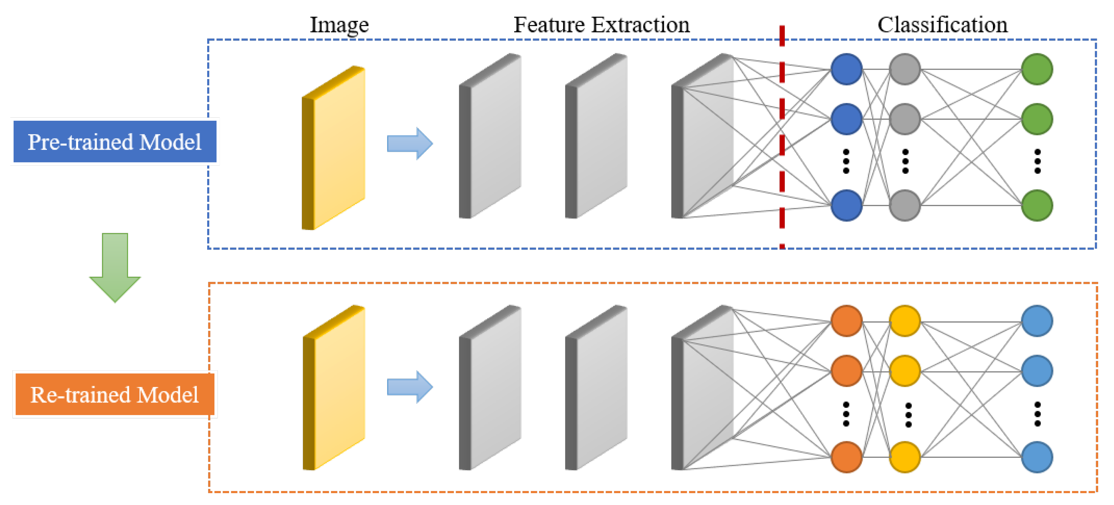
To compensate for the data deficiency, a pre-trained model can be retrained using the available training data. This is because the pre-trained model already contains the information of the extracted features favorably in the weights of the feature extraction layers. However, this method is limited in terms of increasing the classification accuracy, as eventually, it needs to augment the training data to improve its classification performance.
Collecting extensive training datasets is another solution for overcoming the problem of data deficiency. Many researches demonstrated the relationship between the amount of the training dataset and classification accuracy. There are many data augmentation techniques to increase the number of training images. Geometric transformation is usually applied for image data augmentation. However, there are limitations to augmenting the training data via geometric transformation, such as the linearization and standardization of data.
The overall research objective is to recognize and classify ten components for picking, placing, and assembling work. However, this yields data deficiency when training the deep learning network to recognize and classify components because these components are uncommon, as previously mentioned. Therefore, we propose a method for effectively improving the object classification accuracy of the deep learning network in the case of a small dataset in various manufacturing domains. To accomplish the goal of object recognition, even if there are few images, we focus on a method generating the massive training data from image data augmentation methods. Our study makes three main contributions:
the extraction of the target object from the background while maintaining the original image ratio;
color perturbation based on the predefined similarity between the original and generated images because of the decision of the reasonable perturbation range;
data augmentation by combining color perturbation and geometric transformation.
We eliminate the background, extract the target object, generate the image by tuning pixel values, and transform to implement this concept. Mainly, the background is eliminated by considering the characteristics of the CIE L*a*b* color space. Besides, an object in an image is extracted such that it is proportional to the ratio of the object in the original image. Next, we change the image by determining the reasonable range for color perturbation and tuning the pixel values based on color space, following which, we combine the tuned images with the geometric transformations. This is unlike the traditional method, which arbitrarily adds the pixel values to the RGB color space. Subsequently, we train the pre-trained network by using the generated images. This step is called transfer learning. To verify the proposed method, we compare and analyze the experiments with one another in terms of the color perturbation of three color spaces and two geometric transformations. We compare the classification result of the trained networks by using test images.
The rest of this paper is organized as follows. In
Section 2, we introduce works related to data augmentation, color spaces, similarity calculation, and transfer learning. In
Section 3, we discuss the performance of the proposed method that applies deep learning to perform object recognition on a small dataset. In
Section 4, we present the experimental results of the proposed method. Finally, in
Section 5, we provide the conclusions.
3. Proposed Method
As previously mentioned, it is difficult to collect a sufficient amount of training data to apply deep learning because the target object of the manufacturing domain is not generally an uncommon item. This results in a trained classifier that is vulnerable. Therefore, in this study, we propose a method of augmenting the training data to counter data deficiency.
To compensate for the training data deficiency in the manufacturing domain, in this study, we propose a method of augmenting the data using a small dataset by changing the pixel value with respect to color spaces and transforming the image via rotation and flipping. The reason why we selected color perturbation is that the image is closely connected with luminance in the environment, and luminance has an influence on the color of the object in the image. The reason why we selected geometric transformation is that our experiments were conducted on a conveyor.
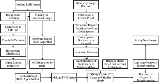
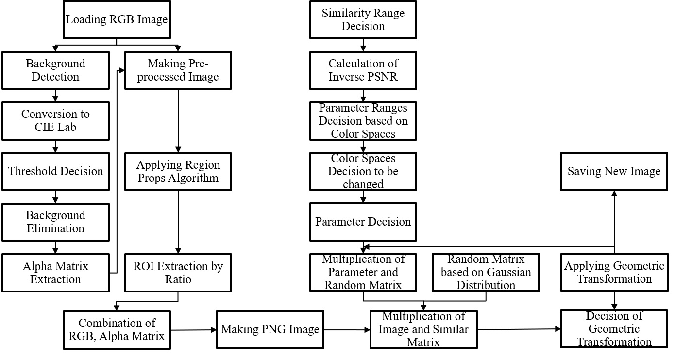
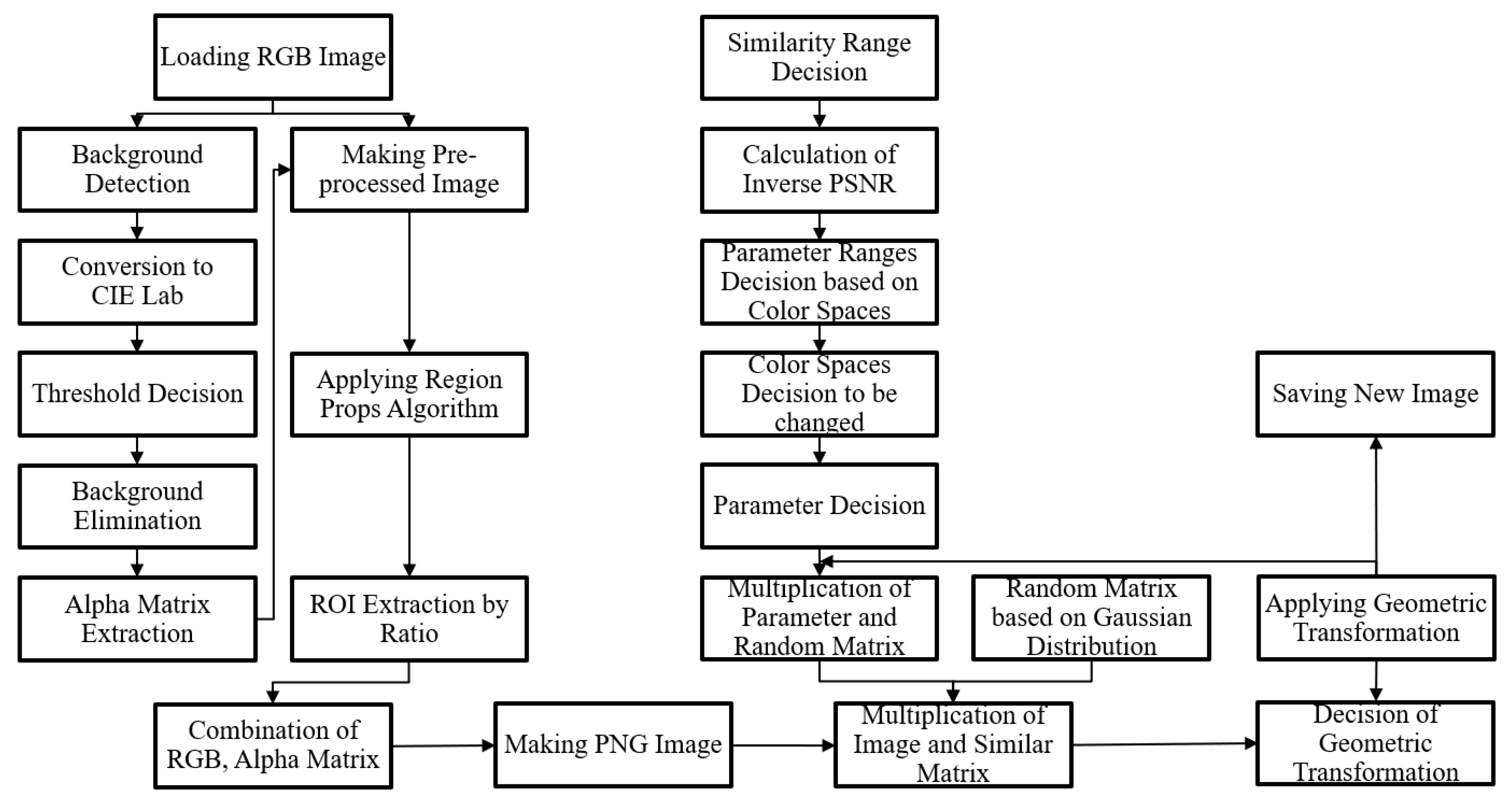
Unlike the traditional method, which randomly adds the values to apply the color perturbation, the proposed method applies the color perturbation based on the decision of a reasonable range, which is determined by the inverse PSNR equation. Furthermore, in case of the traditional method, the input size of the training image for training the deep learning network is just resized by the input size of the network applied for the transfer learning. Therefore, the ratio of the image is distorted, and it results in decreasing the image classification accuracy. Therefore, the proposed method crops and resizes the image by maintaining the ratio of the object size in the original image. To implement this, the center point of the object in the image is calculated. Furthermore, to analyze the effect of the number of training images, the combination of the color perturbation with respect to each color space and the combination of the geometric transformation are conducted. The overview of the proposed method is depicted in
Figure 2. The proposed method is divided into three parts: image pre-processing (background elimination; ROI extraction while maintaining the ratio of the original image size), color perturbation via a random Gaussian distribution based on the inverse PSNR, and geometric transformations.
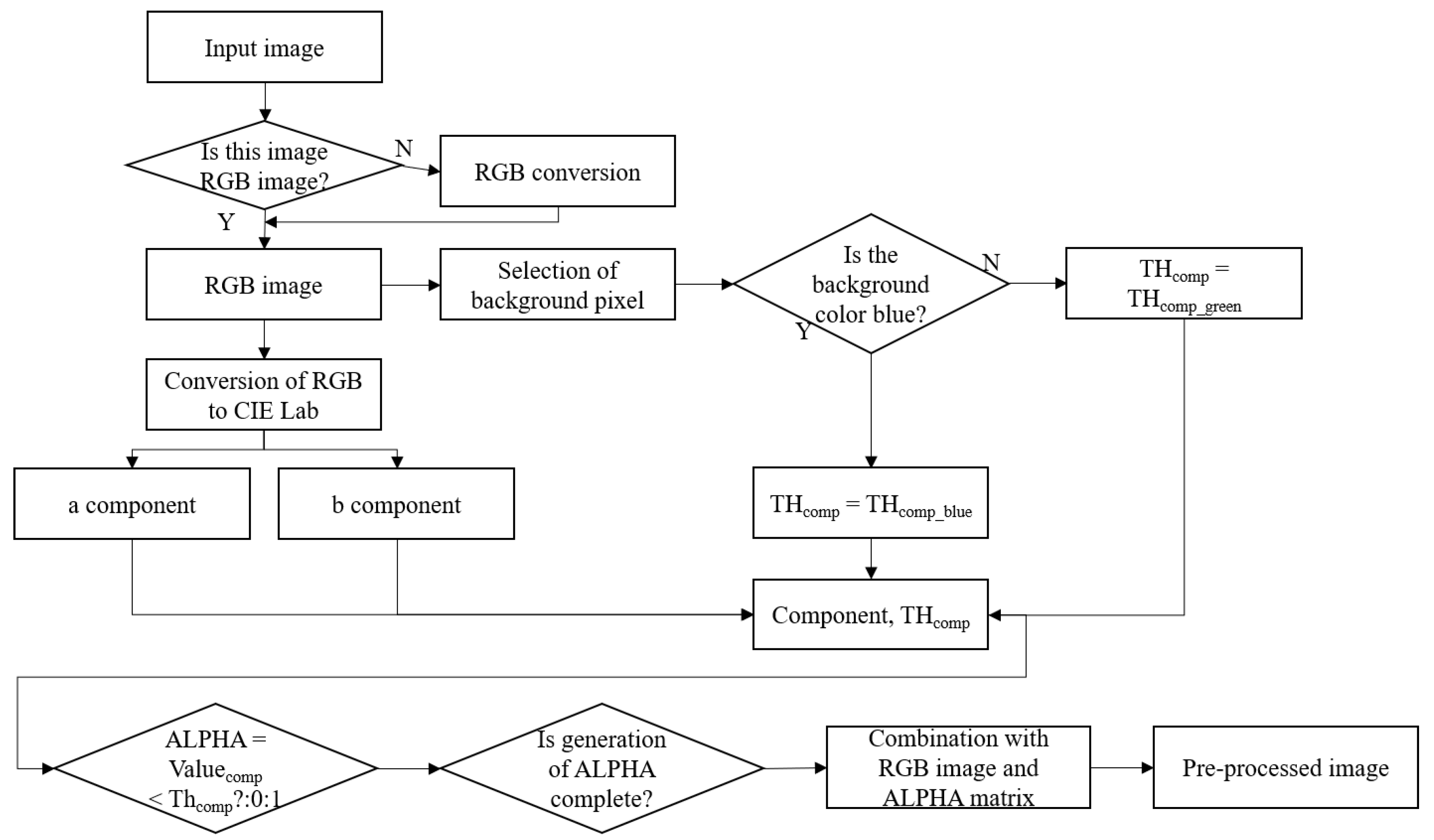
First, we capture the target objects that should be recognized by the deep learning network by using a vision sensor. In this study, the object images were comprised of 32 images for each category. Next, the background is eliminated to improve the classification accuracy by reducing the elements that have an influence on training the object. The objects for the image classification are laid on a color board. An object should be extracted from the image, without the color board as the background image. This step is shown in
Figure 3.
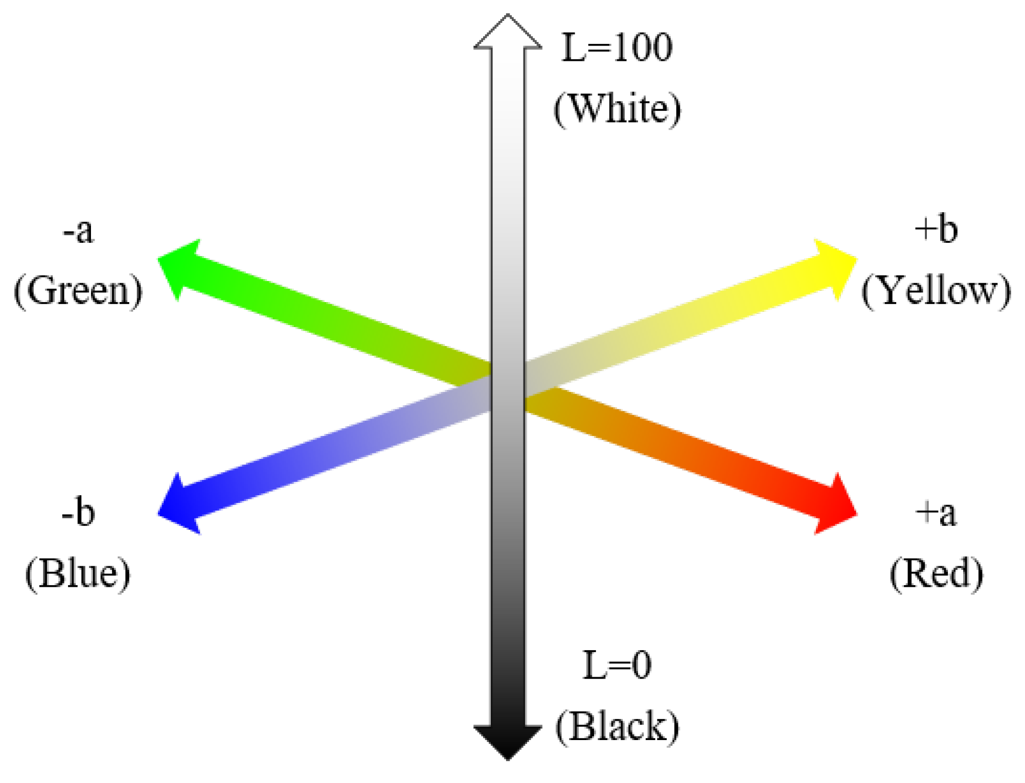
To eliminate the background color, the characteristics of the CIE L*a*b* color space are used. If the background color is white, shadows hinder the background removal process. Therefore, a background with a different color is considered. As previously mentioned, the CIE L*a*b* color space is comprised of the red–green axis and blue–yellow axis, as depicted in
Figure 4.
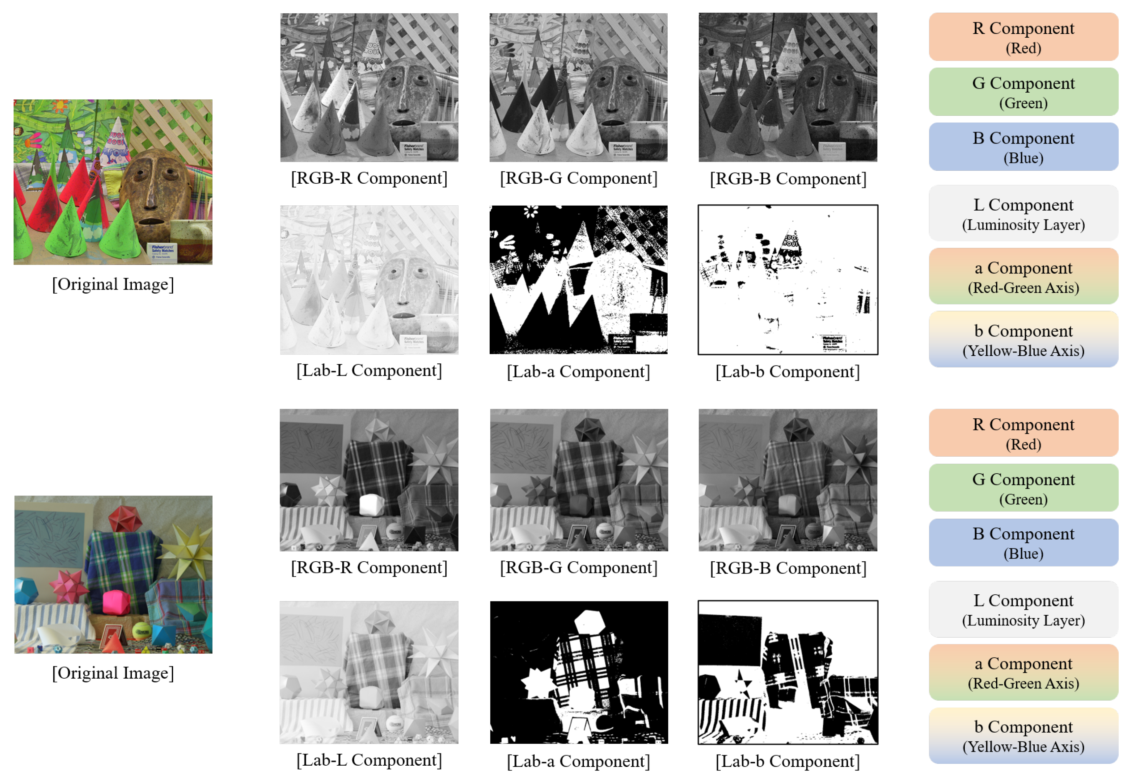
Figure 5 depicts each component of each color space. Red, green, blue, and yellow are more distinct in each component in the CIE L*a*b* color space than the RGB color space [
35,
36]. Using this characteristic, we can easily extract the object from the background color. Because the colors of the object used for image classification are varied, such as red, green, blue, and black, the background colors of the board are determined as green and blue. The green and blue colors can be effectively extracted, as they have convenient values in the CIE L*a*b* color space that help distinguish the colors. The green color is located at the bottom of the a component, which is related to the red–green axis. In addition, the blue value is located at the bottom of the b component, which is related to the blue–yellow axis. Therefore, we selected green and blue colors as the background color. The process for eliminating the background is as follows:
denotes the alpha matrix of the PNG image file. This matrix is related to the transparency of an image. The region that we consider as the background is removed and transparentized using the alpha matrix. The term
denotes a pixel value in each component layer. The component layer is determined as the a component if the background is green color or the b component if the background is blue color. The term
denotes each threshold value with respect to the a or b component layer for extracting the green or blue color. In addition,
is determined according to the characteristic depicted in
Figure 4.
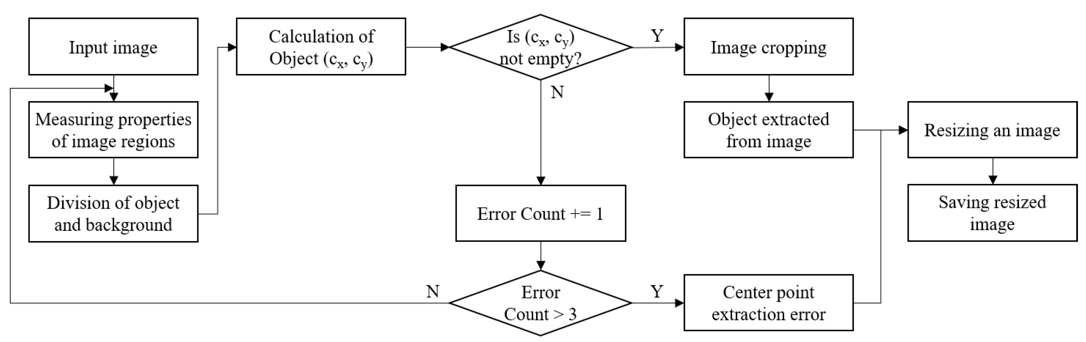
After background elimination, the image is cropped as the original image ratio is maintained as depicted in
Figure 6. The image ratio is important because the distortion affects the classification accuracy during the training of the deep learning network. However, the training images are just resized according to the input size of the network that is used for transfer learning. In this case, the ratio of the image size of the training images is not maintained, and it may result in low classification accuracy. Therefore, we crop and resize the image while maintaining the ratio when extracting the target object from the image. For this procedure, a division algorithm is applied for extracting the object from the background by measuring the properties of the image regions [
37,
38]. The center of an object in an image is calculated by the region propsalgorithm. Then, the image is cropped and resized as the square shape. Its size is determined as the input size of the deep learning network used for training.
Next, the data augmentation is performed after image pre-processing. The main concept of the proposed method is to generate similar images to build an enormous amount of training data from a small amount of original image data. Because the number of training images affects the performance of the image classification that is based on a deep learning network, we must prepare a massive training dataset for training the deep learning network. Although the training data generated using the proposed method should be similar to the original data, they should be nonlinear to ensure the diversity required to train the network effectively. The reason behind considering similarity is that the similarity of training images in the same category should be guaranteed to a certain degree for the satisfactory performance of the classifier. Therefore, we proposed a data augmentation method by generating an image that is similar to the original one on the basis of a similarity calculation. In addition, we focused on color perturbation because color is affected by lighting and can be changed to another color. Therefore, to generate new images reasonably based on the color perturbation for training the network, we attempted to specify the range of transformation. To implement this concept, we considered the method of calculating the similarity between the original image and the generated image. Therefore, we applied the concept of PSNR for data augmentation.
By using (
16) derived from (
13), the similarity between two images can be calculated. Therefore, we induce the method for generating similar images by inversely considering the PSNR equation. First, the range of the PSNR result value is set. Subsequently, by inversely calculating the PSNR equation, the perturbation range of pixel values is determined. Accordingly, a new image dataset that will contain the training data is generated. An image that is similar to the original image should be generated for augmenting the training data. In addition, the pixel values are generally changed because of the lighting in the environment. Therefore, the proposed method considers color perturbation. The inverse PSNR equation is used to realize a reasonable transformation.
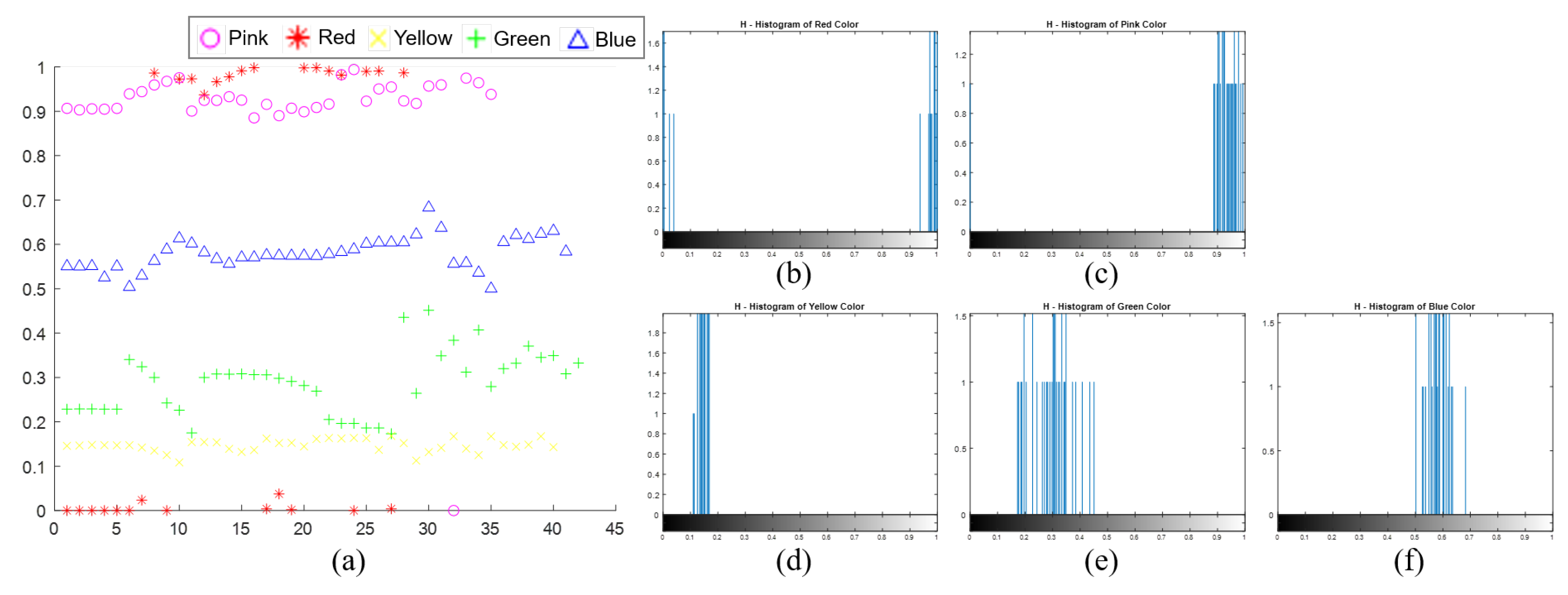
The inverse PSNR can be used to determine the range of the transformation with respect to the color perturbation. To generate a new image while considering its similarity with the original image, the characteristics of the color space are concretely specified. Using the proposed method, the pixel values are tuned over one color space. For reference, the RGB and CIE L*a*b* color spaces have three and two chromaticity layers, respectively, while the HSV color space has only one layer, which is directly related to the chromaticity layer. In the case of HSV color space, it is difficult to distinguish the colors on the boundary as depicted in
Figure 7 [
39]. As depicted in the above figure, although the H value of the pixel is changed slightly, the red color can be shown as pink or otherwise. Furthermore, H values are similar in the case of yellow and green. Therefore, other color spaces for color perturbation should be considered. In the case of the CIE L*a*b* color space, the parts in which the pixels denote red color are distinct in the a-component layer unlike in the L- and b-component layers. The parts in which the pixels denote yellow color are distinct in the b-component layer. Owing to these characteristics of the CIE L*a*b* color space, we applied the RGB, CIE L*a*b*, and HSV color space to perform data augmentation for diverse transformation.
Color perturbation was performed on the basis of inverse PSNR and the characteristics of one, two, and three color spaces. After calculating the inverse PSNR, the matrix of the color perturbation was generated by adding values via the random Gaussian distribution. By determining the range of the perturbation, the interrelated images were generated to be similar to the original images. This affected the classification accuracy by reducing the generation of images as the outlier. Finally, we combined two geometric transformations for augmenting the training data. Because the experimental environment was related to a conveyor, rotation and flipping were applied after the procedure of color perturbation on the basis of the similarity of the generated images with the original images.
Transfer learning was applied to improve the training efficiency. Among the pre-trained networks, the VGGNet network was re-trained using new training images that were generated using the proposed method. We chose VGGNet because, in our previously conducted work, it showed better performance than those of other pre-trained networks.
4. Experimental Results and Discussion
In this study, we proposed a method to improve the image classification accuracy for small datasets. We applied transfer learning because a method that updates the weights of fully connected layers is more effective than one that updates the weights of all the layers of the network [
34].
The aim of the experiment was to classify the objects of 10 categories. Identifying images from these categories is difficult because they are uncommon and not general items, whereas general items are contained in well-known and existing image datasets. Therefore, the training images should be collected first, although significantly few images were manually collected as the training data. The original images were acquired as the training data using the vision sensor. The number of original images was 32 in each category. In addition, the test data were collected in the same manner as before. The test data were not contained in the training dataset. All experimental results were verified with test data, which was not generated arbitrarily and just captured from the vision sensor. Classification accuracy in the tables indicates the results classifying the object of test data.
To verify the proposed method, first we compared the traditional method with the proposed one. Especially, to demonstrate the color perturbation with respect to the characteristic of color spaces and the geometric transformations, we compared and analyzed the experiments of each color space and each geometric transformation.
Table 1 presents the results of image classification by comparing the traditional methods with the methods that apply color perturbation based on the inverse PSNR with respect to three color spaces based on the proposed method.
The traditional methods work by adding random values in the color channels. Traditional Methods #1 and #2 arbitrarily transform the pixel values in terms of the RGB color space. Traditional Method #1 adds positive values, whereas Traditional Method #2 adds positive or negative values. As presented in this table, the case of adding only positive values had better performance compared with the case of adding positive or negative values. RGB PSNR indicates the generated training data by applying color perturbation based on the inverse PSNR with respect to the RGB color space. Lab PSNR represents the generated training data by applying color perturbation based on the inverse PSNR with respect to CIE L*a*b* color space. HSV PSNR denotes the generated training data by applying color perturbation based on the inverse PSNR with respect to HSV color space.
In addition, the methods that apply color perturbation based on the inverse PSNR had better classification accuracy than that of the traditional methods. To conduct the experiments in the same condition, we arbitrarily extracted an equal number of training images with respect to the methods listed in
Table 1. The classification results are presented in
Table 2.
In addition,
Table 2 shows that the methods that applied color perturbation based on inverse PSNR could improve the classification accuracy better compared with the traditional methods. The combination of extracted images was reflected in the classification results. Next, another experiment was performed to compare the cases of joining the training data generated via the inverse PSNR together with respect to each color space. The results are presented in
Table 3.
From
Table 3, it was evident that increasing the number of training images did not always guarantee an improvement to the classifier performance. This was because the classification result obtained upon joining the training data via inverse PSNR in terms of RGB, Lab, and HSV color spaces was 54.0%, while the classification results obtained upon joining two training datasets among the dataset generated via the inverse PSNR in terms of RGB, Lab, and HSV color space had higher performance than 54.0%.
In a previously conducted research, we generated the training dataset by applying Lab PSNR after applying RGB PSNR [
40]. This was because the number of training images was critical for improving the classification accuracy. In addition, in this study, the classification result of combining RGB PSNR + Lab PSNR showed better performance when two training datasets were combined, as presented in
Table 3. Therefore, we performed additional experiments regarding overlapping the inverse PSNR method on two color spaces: the first one (RGB-Lab PSNR) was applying Lab PSNR after applying RGB PSNR; the other one (Lab-RGB PSNR) was applying RGB PSNR after applying Lab PSNR. The reason behind considering the processing order was to ascertain whether the processing order was influential or not. The experimental results are presented in
Table 4.
Comparing
Table 1 and
Table 4, the result obtained upon overlapping the inverse PSNR method on two color spaces was better than that obtained by adding up the three training datasets generated using the inverse PSNR method in terms of each color space. Therefore, we performed the experiment considering the following three categories: the case of the inverse PSNR method on only one color space, the case of adding up the training datasets, and the case of overlapping the inverse PSNR method on two color spaces. As previously mentioned, two geometric transformations, namely flipping and rotation, were applied to each training dataset performed using the inverse PSNR method, as the target experiment was related to the conveyor. First, we applied the flipping method after applying the color perturbation based on the inverse PSNR method. The results are presented in
Table 5.
The experimental results showed that Experiment #4 yielded better performance than the other experiments. The training data were composed by adding the two training datasets generated using the inverse PSNR method with respect to the RGB color space and CIE L*a*b* color space, respectively, and then performing the flipping method (horizontal, vertical, and horizontal–vertical). Although Experiments #5, #6, #7 had more training data than that of Experiment #4, they showed lower performance regarding test data. This meant that the number of training datasets was not the only reason for the improvements in the classification results. With a sufficient amount of training data, the data should be effectively augmented to train the network. Next, we applied the rotation method as another geometric transformation to the training dataset. The results are presented in
Table 6.
From
Table 6, it is evident that applying the rotation method could significantly improve the classification accuracy. Because the objects were randomly laid down with respect to the rotation angle of the object in the conveyor environment, the rotation method was more influential than the flipping method. In this case, Experiment #6, which was related to overlapping the inverse PSNR method about two color spaces, had higher performance. In addition, we applied the flipping and rotation methods together, and the results are presented in
Table 7.
In the case of applying the flipping and rotation methods together, the performances of the trained networks slightly increased. In this case, the trained network of Experiment #4 by the training dataset adding up the two training data generated by the inverse PSNR method with respect to the RGB color space and CIE L*a*b* color space and performing the flipping method (horizontal, vertical, horizontal-vertical) had higher performance than those of others, as in
Table 3 and
Table 5.
Finally, we performed additional experiments by using an equal amount of training data. The smallest number of the generated training images was 1152 in the case of applying the color perturbation based on the inverse PSNR method with respect to the RGB color space and flipping transformation. Therefore, one-thousand training images were arbitrarily extracted in each category and used for training the network in the same manner as before. The experimental results are presented in
Table 8.
Because the amount of training data was reduced, the results of the classification accuracy tended to be slightly different than before. The experiment with the best performance with respect to average classification accuracy, as shown in
Table 8, was the one in which the inverse PSNR method was applied in terms of overlapping CIE L*a*b* and RGB color space and rotation. The average classification accuracy was 92.0%, and the variance of the classification accuracy calculated using (
17) was four. The experiment in which the inverse PSNR method was applied in terms of RGB and CIE L*a*b* color spaces and rotation achieved the second best performance. The average classification accuracy was 91.7%, and the variance of the classification accuracy calculated using (
17) was 2.3.
For the experimental results, we generally considered the best case wherein rotation and flipping were applied after the color perturbation with RGB and CIE L*a*b* color spaces by using the inverse PSNR. In addition, the results obtained using the proposed method applied to
Table 7, which showed higher accuracy, tended to be similar to or lower than those of the proposed method applied to
Table 6. In the case of applying the inverse PSNR method in terms of the RGB and CIE L*a*b* color spaces and two geometric transformations, the variance of the classification accuracy was 14.3. This meant that the classification accuracy was heavily influenced by the randomly extracted training data. In addition, the figure below shows that, as mentioned earlier, a sufficient amount of training dataset increased the classification accuracy.
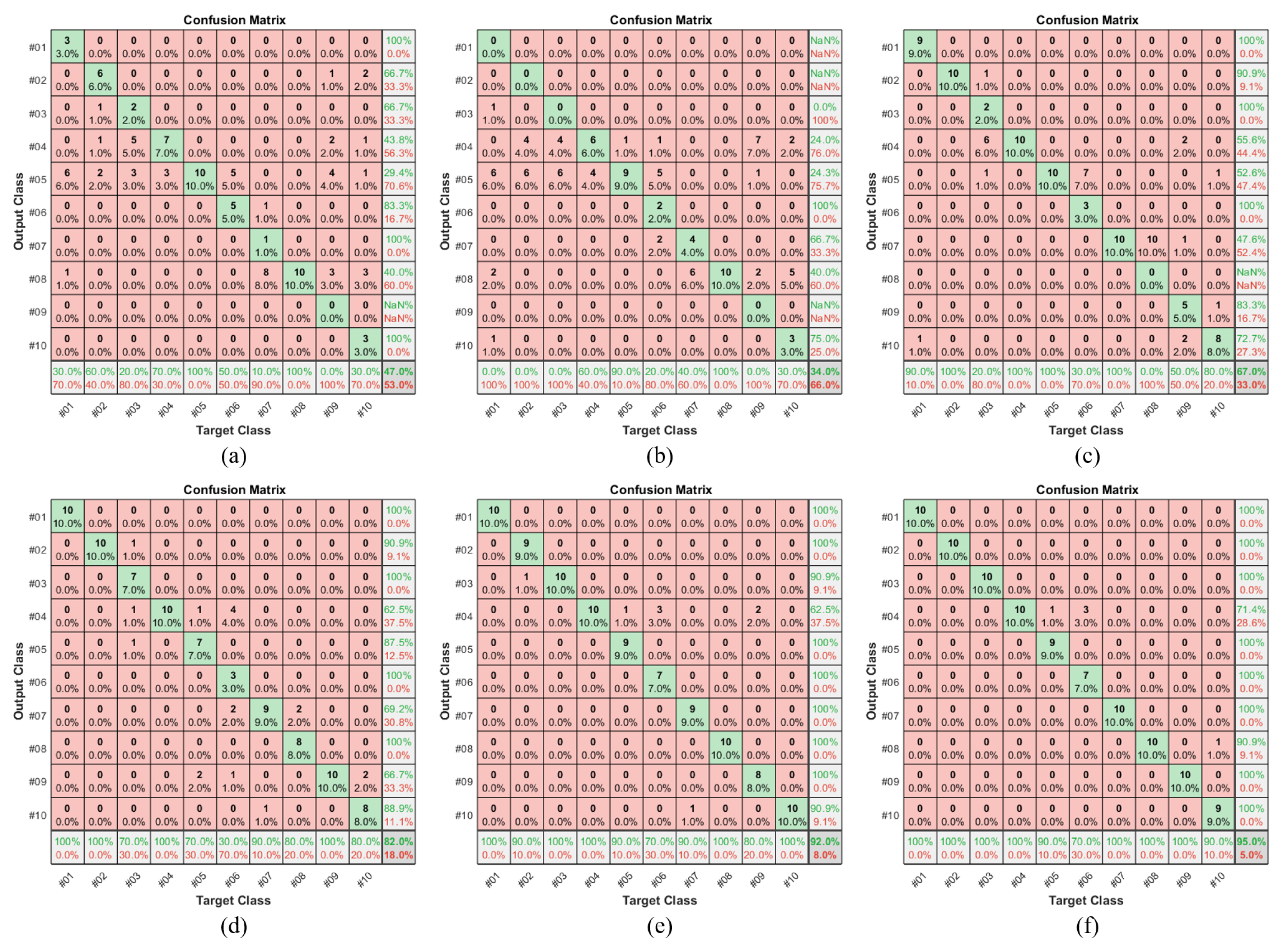
In
Figure 8, we compare the cases of using the traditional methods and the case of applying geometric transformation based on RGB PSNR + Lab PSNR training data, which was mostly the best case among the training data generated by the proposed method. The classification accuracy for Object #3 gradually increased in sequence. From
Figure 8a,b, it was evident that the classification results were mostly misclassified to be of some output class. In the case of
Figure 8c, Object #3 was mostly classified as Object #4. Their shapes were similar to a rectangle. By applying geometric transformations, the amount of the training data and the classification accuracy increased. Finally, Object #3 could be classified 100% using the re-trained classifier. In addition, Object #6 was mostly classified as Object #5, as depicted in
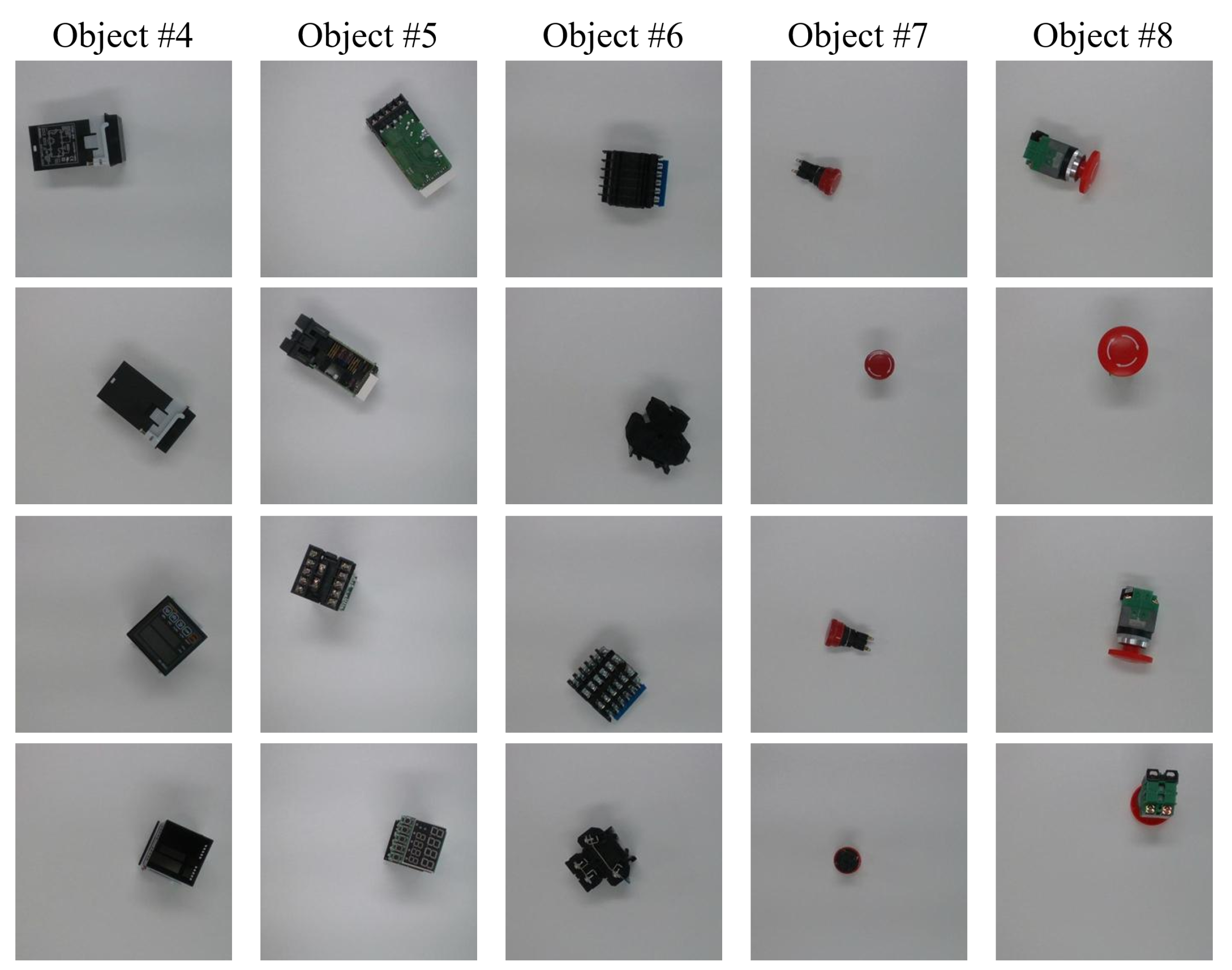
Figure 8c. As depicted in
Figure 9, Objects #4, #5, and #6 were significantly similar, especially when they were laid down in a standing position. However, using the proposed method, the classification accuracy for Object #6 could be improved. Because Object #8 was significantly similar to Object #7, as depicted in
Figure 9, Object #8 was classified as Object #7, as depicted in
Figure 8c. However, Object #8 could be classified 100.0% using the proposed method. Similarly, Object #9 was misclassified as Object #10, which was similar to Object #9. However, the proposed method could classify Object #9 with 100.0% accuracy.
5. Conclusions
In this study, we proposed a method to overcome data deficiency and improve classification accuracy. Accordingly, we eliminated the background color and extracted the object while maintaining the original image ratio. In addition, new training images were generated via color perturbation based on the inverse PSNR with respect to color spaces and geometric transformations.
Experiments were performed to demonstrate the reasonable combination by considering color spaces and geometric transformations and their combinations, respectively. First, we composed 11 training datasets to verify the validity of range determination for color perturbation: Traditional Method #1, Traditional Method #2, RGB PSNR, Lab PSNR, HSV PSNR, RGB PSNR + Lab PSNR, Lab PSNR + HSV PSNR, RGB PSNR + HSV PSNR, RGB PSNR + Lab PSNR + HSV PSNR, RGB-Lab PSNR, Lab-RGB PSNR. Traditional Methods #1 and #2 were related to adding the pixel values of the RGB color space arbitrarily. The other datasets were related to the proposed method. The experimental results showed that the classification accuracy could be improved by the proposed method as compared with the traditional methods, and the RGB PSNR + Lab PSNR training dataset showed better performance than the others.
Second, we composed 21 training datasets to verify the effectiveness of geometric transformations: flipping with RGB PSNR, flipping with Lab PSNR, flipping with HSV PSNR, flipping with RGB PSNR + Lab PSNR, flipping with RGB PSNR + Lab PSNR + HSV PSNR, flipping with RGB-Lab PSNR, flipping with Lab-RGB PSNR, rotation with RGB PSNR, rotation with Lab PSNR, rotation with HSV PSNR, rotation with RGB PSNR + Lab PSNR, rotation with RGB PSNR + Lab PSNR + HSV PSNR, rotation with RGB-Lab PSNR, rotation with Lab-RGB PSNR, flipping and rotation with RGB PSNR, flipping and rotation with Lab PSNR, flipping and rotation with HSV PSNR, flipping and rotation with RGB PSNR + Lab PSNR, flipping and rotation with RGB PSNR + Lab PSNR + HSV PSNR, flipping and rotation with RGB-Lab PSNR, flipping and rotation with Lab-RGB PSNR. The experimental results showed that the RGB PSNR + Lab PSNR with rotation and flipping method showed better performance in the training data generated by the proposed method.
The classification accuracy of the network trained using the generated dataset by color perturbation based on the similarity calculation, which was related to our contribution, showed better performance than the arbitrary color perturbation like the traditional methods. In general, the numerous image data showed a better performance of the classification accuracy. However, it was not absolute. Therefore, we plan to study effective data augmentation methods by evaluating the appropriate numerical value for improving the performance of the classification accuracy.
The experimental results showed that the proposed method could improve the classification accuracy by classifying similar objects, which were easy to misclassify. This indicated that color perturbation based on similarity was effective at improving the classification accuracy. In future work, we plan to develop other reasonable data augmentation methods to overcome data deficiency, including in the manufacturing domain.


