Robust Space Time Adaptive Processing Methods for Synthetic Aperture Radar

Abstract

This paper proposes two modified space time adaptive processing (STAP) methods based on piecewise sub-apertures and data constraints for non-stationary interference cancellation in synthetic aperture radar (SAR) applications. In these methods, the entire synthetic aperture time is divided into several sub-apertures so that the interference can be considered as stationary in each sub-aperture. At the same time, the consistency of the echo phase in the slow time domain is preserved by the data constraint to ensure the null depth of the antenna pattern for non-stationary interference cancellation and the performance of azimuth focusing in SAR. The proposed algorithms are validated through the model simulation and measured data.

1. Introduction

Synthetic aperture radar (SAR) has been more and more widely used in civilian and military fields [1,2,3]. Along with growing crowdedness of the electromagnetic spectrum and rapid development of SAR interference technology [4,5,6,7], SAR is now faced with increasingly serious unintentional or intentional interference, and the algorithm of interference cancellation in SAR has received growing attention in recent years.

The common methods of interference cancellation in SAR can be divided into two categories. One is to utilize the difference between the interference and radar echo in the time domain or frequency domain so that the interference cancellation can be realized through filters in the time or frequency domain. This includes the classical frequency notch method and the time-frequency filtering method [8,9]. Some advanced methods based on short-time Fourier transform, wavelet transform, empirical mode decomposition, eigen subspace filtering and independent component analysis (ICA) [10,11,12,13,14] have also been proposed. These methods not only cause certain loss to the echo signal itself, but also cannot effectively suppress intentional interference from jammers such as wide-band noise jamming or dense repeater jamming. Another kind of method is based on digital array processing with multi-channels, using adaptive digital beam forming (ADBF) or the space time adaptive process (STAP) algorithm for interference cancellation [15,16,17]. Multi-channels in the SAR can be used to form a beam in the direction of the desired ground returns and to steer a null in the direction of the interference simultaneously. With the rapid development of the multi-channel SAR system and the improvement of digital signal processing, these methods have shown more and more advantages with regards to excellent performance, wide application and high flexibility.

Moving target indication (MTI) is a common radar mission involving the detection of airborne or surface moving targets. To detect moving targets in the background of clutter and interference, it is necessary to suppress clutter and interference by various methods. Single-channel techniques that exploit the Doppler spectrum or the short time Fourier transform are used in general for static clutter discrimination from moving targets. In multi-channel systems, STAP is an advanced multi-channel adaptive processing technique used for clutter mitigation and interference cancellation purposes and has been widely treated for general airborne radar [18,19]. Furthermore, the STAP technique has also been introduced into the SAR system for both clutter suppression and high resolution imaging of moving targets [20,21]. The typical application of STAP in airborne radar is the ground moving target indication (GMTI) mode, and the coherent processing interval (CPI) of the GMTI mode is only tens of milliseconds. It can be considered that the direction of arrival (DOA) from the jammer is constant in the CPI, which means the interference is stationary. Since the CPI in SAR is usually more than a few seconds, due to the high speed motion of the platform, the DOA of the jammer is time-varying, which means the interference is non-stationary in the CPI. There are two main kinds of methods for non-stationary interference cancellation. One is to widen the null width near the interference’s DOA in the adapted beam pattern by digital array processing [22], but this may lead to a loss in the depth of the nulls. The other method for non-stationary interference cancellation is time-varying STAP [23,24], which means using different adaptive weight vectors for each pulse. However, due to the deformation of the beam pattern from pulse to pulse, the SAR echo would be modulated in the slow time domain, resulting in the degradation of the azimuth focusing performance.

In this paper, we propose two STAP methods for SAR with piecewise sub-apertures and data constraints for non-stationary interference cancellation based on element space processing and the generalized sidelobe canceller (GSC), respectively. In these methods, the entire synthetic aperture time is divided into several sub-apertures so that the interference can be considered as stationary in each sub-aperture. At the same time, the consistency of the echo phase in the slow time domain is preserved by the data constraint to ensure the null depth of the antenna pattern for non-stationary interference cancellation in the entire synthetic aperture time and the performance of azimuth focusing in SAR. The proposed algorithms are validated through the model simulation and measured data.

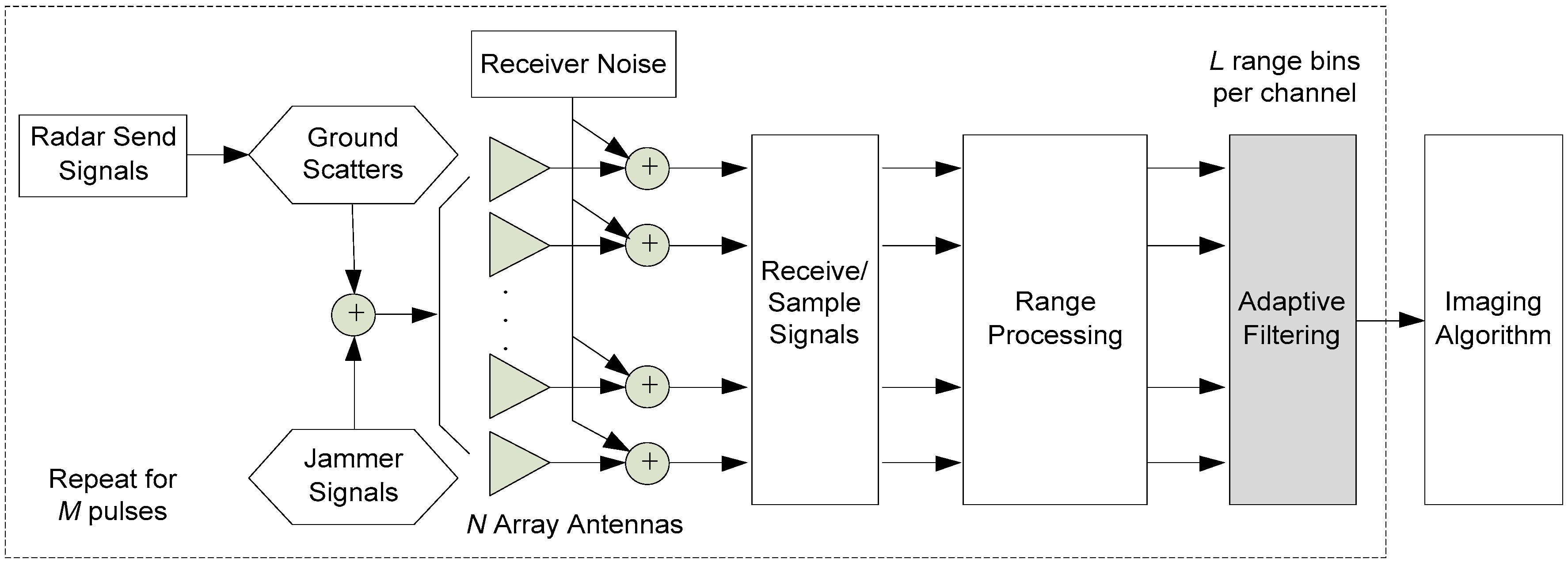
2. SAR Simulation Models

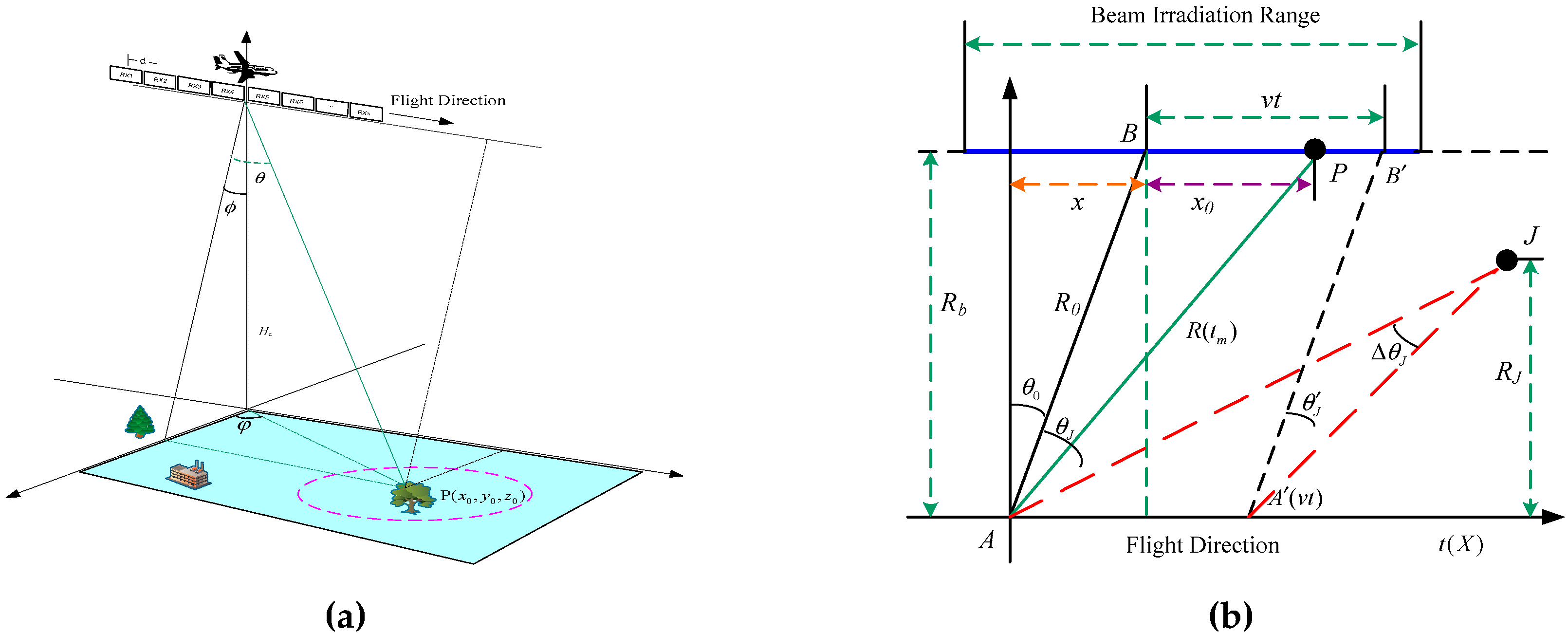
2.1. SAR Signal Model

Consider a multi-channel SAR system of a linear antenna array with N equi-spaced receiver channels along the azimuth direction. Figure 1 is the geometric diagram of the multi-channel SAR. Suppose all the channels and targets are located in the three-dimensional (3D) Descartes coordinate system. The radar platform travels along the X-axis at v m/s. Figure 1a shows the 3D geometric model, where H_c represents the height of the platform, the φ represents the azimuth angle, the ϕ represents the elevation angle, and the θ is the squint angle. Figure 1b shows the diagram of the geometry relationship in the slant plane, where the blue lines show the beam irradiation range when the radar is at point A, and point B is the position of the beam center. When the point target is located at the center of the beam, R₀ is the distance between the target and the receiver channel, and θ₀ represents the cone angle corresponding to the beam center. When the radar moves to the point A′, the point B′ is the center of the beam.

The radar transmits a linear frequency modulated (LFM) signal and the received echo of the nth channel is base-banded and sampled, which can be written as:

$$s(n,\widehat{t},t_m)=\exp \left[j2\pi \frac{(n-1)d\sin {\theta }_0}{\lambda }\right]\cdot A\mathrm{rect}\left(\widehat{t}-\frac{2R(t_m)}{c}\right)\exp \left[j\pi \gamma {\left(\widehat{t}-\frac{2R(t_m)}{c}\right)}^2\right]\exp \left[-j\frac{4\pi }{\lambda }R(t_m)\right]$$

(1)

where A is the amplitude of the target echo, c is the velocity of light, λ is the wavelength, $\widehat{t}$ is fast-time corresponding to the sample in the range domain of a single pulse, $t_m$ is slow-time used to mark different pulses during the pulse string process with the interval of the pulse repetition interval (PRI), T_p is the pulse width, γ is the frequency rate of the LFM signal, B = γT_p is the signal bandwidth, and n refers to the nth channel of the multi-channel receiver. The first exponential term represents the phase difference of the echo between the receiver channel N and channel 1. According to the geometric relation in Figure 2, the instantaneous slant distance between the carrier and the point target P can be obtained:

$$R(t_m)=\sqrt{{(v{t}_m-X_n)}^2+R_b^2-2R_b(v{t}_m-X_n)\sin \theta }\hspace{1em}{X}_n-\frac{L}{2v}\le t_m\le X_n+\frac{L}{2v}$$

(2)

where $v$ is the velocity of the SAR platform, $X_n$ is the azimuth coordinates of a scattering point on the ground, L is the synthetic aperture length, R_b represents the shortest distance between the target and the trajectory of the radar.

After the pulse compression processing in the range domain, and the envelope difference of the echo is neglected, so the echo signal can be expressed as:

$$s(n,\widehat{t},t_m)=\exp \left[j2\pi \frac{(n-1)d\sin {\theta }_0}{\lambda }\right]\cdot \sin \mathrm{c}\left[B(\widehat{t}-\frac{2R(t_m)}{c})\right]\exp \left[-j\frac{4\pi }{\lambda }R(t_m)\right]$$

(3)

2.2. Jammer and Noise Models

For simplicity, consider that the jammer is located at position J in Figure 2b with the cone angle theta θ_J, and the minimum distance from the platform flight trajectory to the jammer is R_J. Assuming the interference signal received by channel 1 of the radar is I₀, the total return for the SAR can be written in matrix form as follows:

$$X(t)=s(t)\cdot a({\theta }_0)+I_0(t)\cdot a({\theta }_J)+N(t)$$

(4)

$$a({\theta }_0)=\left\{1,\exp \left[j2\pi \frac{(2-1)d\sin {\theta }_0}{\lambda }\right],\dots ,\exp \left[j2\pi \frac{(N-1)d\sin {\theta }_0}{\lambda }\right]\right\}$$

(5)

$$a({\theta }_J)=\left\{1,\exp \left[j2\pi \frac{(2-1)d\sin {\theta }_J}{\lambda }\right],\dots ,\exp \left[j2\pi \frac{(N-1)d\sin {\theta }_J}{\lambda }\right]\right\}$$

(6)

where a(θ₀) is the steering vector of the signal echo, a(θ_J) is the steering vector of interference, and N(t) is the receiver noise matrix.

2.3. Basic STAP Method

The covariance matrix of the array received signal is estimated through finite snapshots [25], assuming the snapshot number is L, then the estimator of the covariance matrix from the received signal:

$$\widehat{R}=\frac{1}{L}{\displaystyle \sum _{i=1}^{L}X(i)X^H(i)}$$

(7)

Here, H denotes the Hermitian transpose operator. Then the adaptive filtering is based on the minimum variance distortionless response (MVDR) criterion as follows:

$$\{\begin{array}{c}\min (w^H{R}_{1}w)\begin{array}{cc}& \end{array}\\ \begin{array}{cc}s.t& w^{H}a({\theta }_0)=1\end{array}\end{array}$$

(8)

The equation aims to get the adaptive weight vector w for the minimum output power of the array under the constraint of keeping the output constant and can be solved using Lagrange multipliers [25]. The entire signal process flow of the multi-channel SAR is shown in Figure 2.

2.4. Influence of Platform Motion

Consider a jammer is located at point J when the radar is located at point A, and the relative angle between the jammer and the beam center of the radar is ${\theta }_J$. When the radar moves to point A′, the relative angle between the jammer and the beam center of the radar is ${{\theta }^{\prime }}_J$. According to the geometric relationship in Figure 2b, the difference of the angles is $\mathsf{\Delta }{\theta }_J$, which can be approximated as:

$$\mathsf{\Delta }{\theta }_J\approx \frac{V_{c}t\cos {\theta }_J}{R_J}$$

(9)

For the conventional mode in airborne radar, the CPI is only about tens of milliseconds, so $\mathsf{\Delta }{\theta }_J$ is very small and can be ignored. However, the synthetic aperture time of SAR is usually a few seconds. Consider the situation with the flight speed 150 m/s, synthetic aperture time of 5 s, oblique distance R₀ = 40 Km, and the azimuth angle of jammer 45° as an example. It can be calculated that the direction of interference relative to the platform changes up to 1.5° in the synthetic aperture time, which cannot be ignored for the STAP process. In other words, the interference is time-varying and non-stationary in the synthetic aperture time.

Some different methods for non-stationary interference cancellation have been proposed in the literature. The first method is to select interference samples in the whole synthetic aperture time to get the adaptive weight vector with widen null by STAP directly. Higher spatial freedom of the system is needed in this method, and STAP processing cannot be carried out pulse by pulse, which greatly improves the resources of storage and consumption in the system. The second way is to form a wide null in the beam pattern in the STAP process through the null broadening algorithm [22]. A common problem is that the null depth would be usually reduced or form wide nulls that would raise the sidelobe level or broaden the main beam at the same time. The third method is to suppress the non-stationary interference by dividing the coherent integration time into several batches and using different adaptive weight vectors for each batch [23,24]. In STAP processing, although the mainlobe can be maintained by imposing a single constraint in the desired direction, this may still cause some variations in the beam pattern depending on the differences in the strength or direction of the interference from pulse to pulse, especially for strong interference near the mainlobe, thereby undermining the consistency of the echo phase between batches and leading to degradation of azimuth focusing in the SAR image. To solve these problems, two modified STAP methods for SAR with piecewise sub-apertures and data constraints for non-stationary interference cancellation are proposed in Section 3 and Section 4.

3. The Piecewise Constrained STAP Based on Sub-Apertures Framework

The synthetic aperture time may be partitioned into M sub-apertures containing Q pulses (M = P / Q) and the adaptive weight vectors w_m for m = 1,2,···,M can be updated in each sub-aperture. The essence of the algorithm is to update the adaptive weight vector by subdividing the aperture to adapt to the changes of interference spatial non-stationarity, considering the DOA is stationary in the non-overlapping sub-apertures.

In conventional sub-aperture processing, the adaptive weight vector of each sub-aperture is calculated according to (8):

$$w_m={[v^H(\theta )R_m^{-1}v(\theta )]}^{-1}{R}_m^{-1}v(\theta )$$

(10)

where R_m is the covariance matrix obtained from the interference samples in sub-apertures, w_m is the adaptive weight vector of each sub-aperture and is used to beamform the multi-channel echo data of each sub-aperture respectively. It should be noted that the training data used to estimate the covariance matrix must be target-free in order to avoid the self-cancellation of the target itself [26,27]. A low repetition frequency waveform is usually used in SAR, which means that the range is not ambiguous, so the training data can be sampled before the effective echo reaches the radar receiver in the fast time domain to obtain the target-free samples. Moreover, in order to estimate the covariance matrix accurately, it is necessary to have an adequate number of training data. In SAR, the sampling rate is relatively high. Therefore, it is easy to obtain enough interference samples to estimate the covariance matrix.

The disadvantage of this method is discussed in Section 2. With different adaptive weight vectors in each sub-aperture, although the beam center of the mainlobe can be maintained by the constraint in the look direction, there are still variations in the other parts of the patterns in the mainlobe. The deformation of the antenna patterns would lead to the undermining of phase consistency in the slow time domain between the sub-apertures, which affect the azimuth resolution of the SAR images.

Therefore, a sub-aperture STAP algorithm with data constraint is proposed. In this method, the adaptive weight vectors are calculated in each sub-aperture respectively, and the phase consistency in the slow time domain can be maintained by data constraints, so the azimuth resolution of SAR can be ensured while effectively suppressing the time-varying interference.

In the first sub-aperture, the adaptive weight vector is obtained by the conventional method according to (10), and then the weight vector w₁ can be used to beamform the array echo in the first sub-aperture.

$$w_1={[v^H(\theta )R_1^{-1}v(\theta )]}^{-1}{R}_1^{-1}v(\theta )$$

(11)

In the second sub-aperture, the data constraint condition is added, which permits the vector to change for interference cancellation while guaranteeing that it would not affect the beamform output of the target echo in the second sub-aperture. In order to reduce the amount of computational complexity, in practice, only L pulses at the junction of two sub-apertures need to be selected to constrain the consistency of the echo. Then the constrain can be described as follows [23]:

$$w_1^{H}x(t)=w_2^{H}x(t),t=Q-L/2+1\cdot \cdot \cdot Q+L/2$$

(12)

It can be approximately considered that $w_1^{H}x(t)\approx w_1^H\mathrm{s}(t),w_2^{H}x(t)\approx w_2^H\mathrm{s}(t).$ Because the range bin numbers of each pulse are more than thousands in SAR, only range bins containing strong feature points need to be selected as constraints to reduce the computational complexity. The detection of range bins containing strong feature points can be performed in the fast time domain after the pulse compression process.

The calculation of w₂ is formulated as:

$$\min w_2^H{R}_2{w}_2\hspace{1em}subject to\hspace{1em}{w}_2^H{C}_2=f_2$$

(13)

$$C_2=[v(\theta ),x(Q-L/2+1),\cdot \cdot \cdot x(Q+L/2)]$$

(14)

$$f_2=[1,w_1^{H}x(Q-L/2+1),\cdot \cdot \cdot w_1^{H}x(Q+L/2)]$$

(15)

The solution of (13) is:

$$w_2=R_2^{-1}{C}_2{[C_2^H{R}_2^{-1}{C}_2]}^{-1}{f}_2$$

(16)

The adaptive weight vectors in the remaining sub-apertures can be obtained similarly:

$$w_m=R_m^{-1}{C}_m{[C_m^H{R}_m^{-1}{C}_m]}^{-1}{f}_m$$

(17)

$$C_m=[v(\theta ),x(Q(m-1)-L/2+1),\cdot \cdot \cdot x(Q(m-1)+L/2)]$$

(18)

$$f_m=[1,w_{m-1}^{H}x(Q(m-1)-L/2+1),\cdot \cdot \cdot w_{m-1}^{H}x(Q(m-1)+L/2)]$$

(19)

Then the SAR image can be obtained by two-dimensional processing of the entire aperture data containing all sub-apertures with classical SAR algorithms.

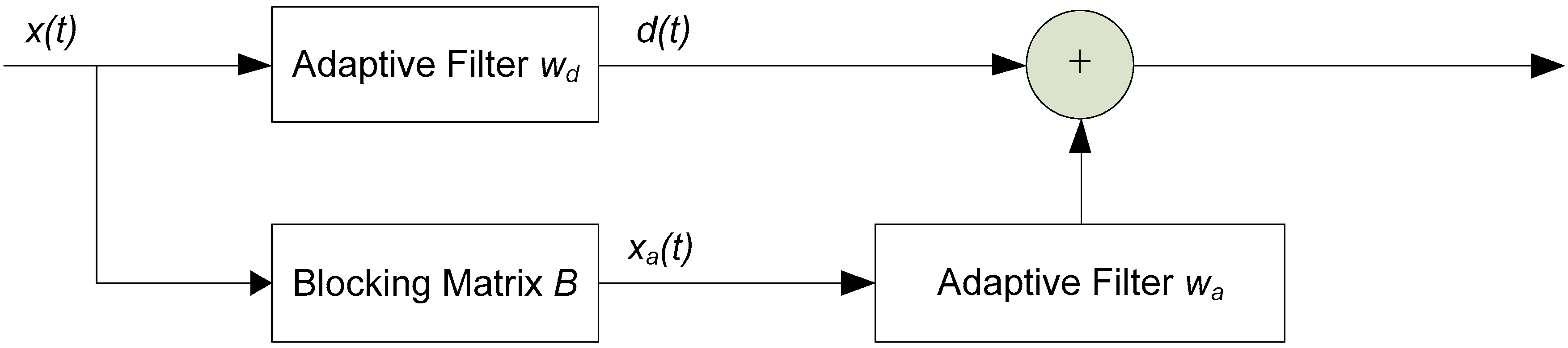
4. The Piecewise Constrained Generalized Sidelobe Canceller

Element space processing is a method of implementing STAP in the spatial frequency domain, and STAP can also be implemented as a generalized sidelobe canceller (GSC), which is equivalent to what element space approaches under ideal conditions [28]. This section presents a modified method of applying piecewise constraints to the GSC (PC-GSC) based on the same idea as Section 3.

The processing flow of the GSC is shown in Figure 3, two processing paths are formed with the main beam d(t) in the desired direction and the reference beam x_a(t) formed by a transformation of the main beam with a blocking matrix B to remove the desired signal from the original echo data. The fixed weight vector of the upper processing path is given by w_s = a(θ₀), where θ₀ is the DOA of the desired target direction.

The signal x_a(t) in the lower processing path then goes through an adaptive filter w_a to minimize the total output power, and is then subtracted from the main beam d(t). To mitigate the spatially nonstationary interference in SAR, piecewise adaptive processing is employed. If the aperture time is partitioned into M data sub-apertures, each of which consists of Q pulses (M = P / Q), the adaptive weight vectors w_a (m), m = 1,2,···,M for the lower processing path in the GSC can be updated in each sub-aperture. The adaptive weight vectors w_a(m) are designed to minimize the scalar mean square error (MSE) of the difference between the upper and the lower processing path, which is given by the following formulation [24].

$$\min E({\left|d(t)-w_a^H(m)x_a(t)\right|}^2)$$

(20)

t = (m − 1)Q + 1,...,mQ and m = 1,2,···,M. d(t) is the output of the upper processing path of the GSC and x_a(t) is the N_a-dimensional data vector for the lower processing path of the GSC.

The weight vector of the upper processing path of the GSC structure is fixed. The adaptive weight vector w_a (m) in the lower processing path needs to be changed in each sub-aperture. To alleviate the temporal modulation introduced by the varying w_a (m), constraints on the adaptive weight vectors w_a (m), m = 1,2,···,M are required. Similar to (18), we define the vector as:

$$C_m={[x(Q(m-1)-L/2+1),\cdot \cdot \cdot x(Q(m-1)+L/2)]}^H$$

(21)

Then the following constraints on the adaptive weight vector are used:

$$w_a^H(m)C_m=w_a^H(m-1)C_m\hspace{1em}m=2,3,\cdot \cdot \cdot ,M$$

(22)

The adaptive weight vector w_a (1) in the first sub-aperture is calculated using (11) without any constraint. The solution to (20) is

$$w_a(m)=R_{xx}^{-1}(m)r_{xd}(m)-{(C_m^H{R}_{xx}^{-1}(m)C_m)}^{-1}[R_{xx}^{-1}(m)r_{xd}(m)-w_a(m-1)]$$

(23)

R_xx(m) is the spatial covariance matrix of the lower processing path of the GSC, and r_xd (m) is the cross-correlation vector between the lower and the upper processing path of the GSC.

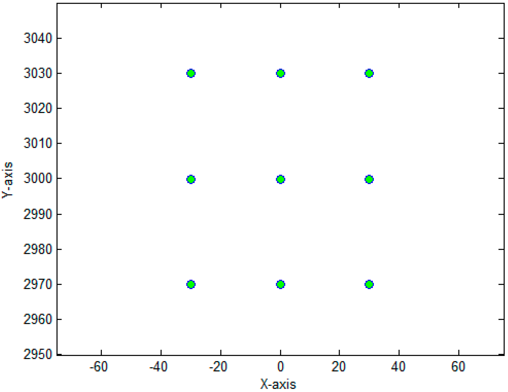
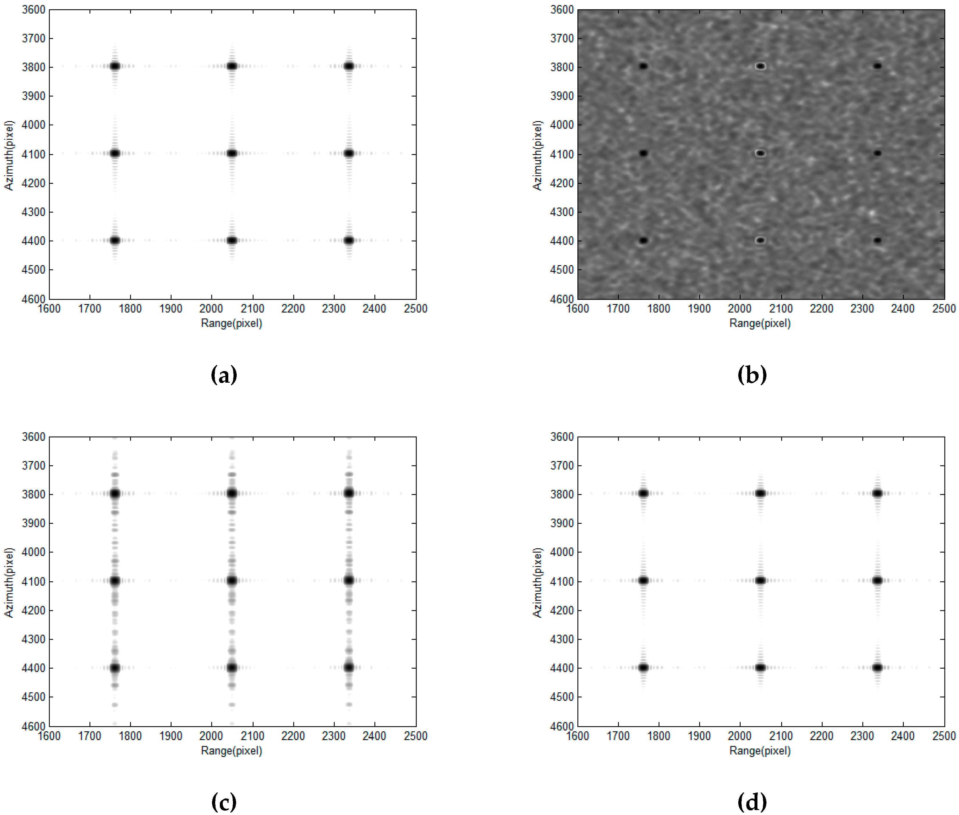
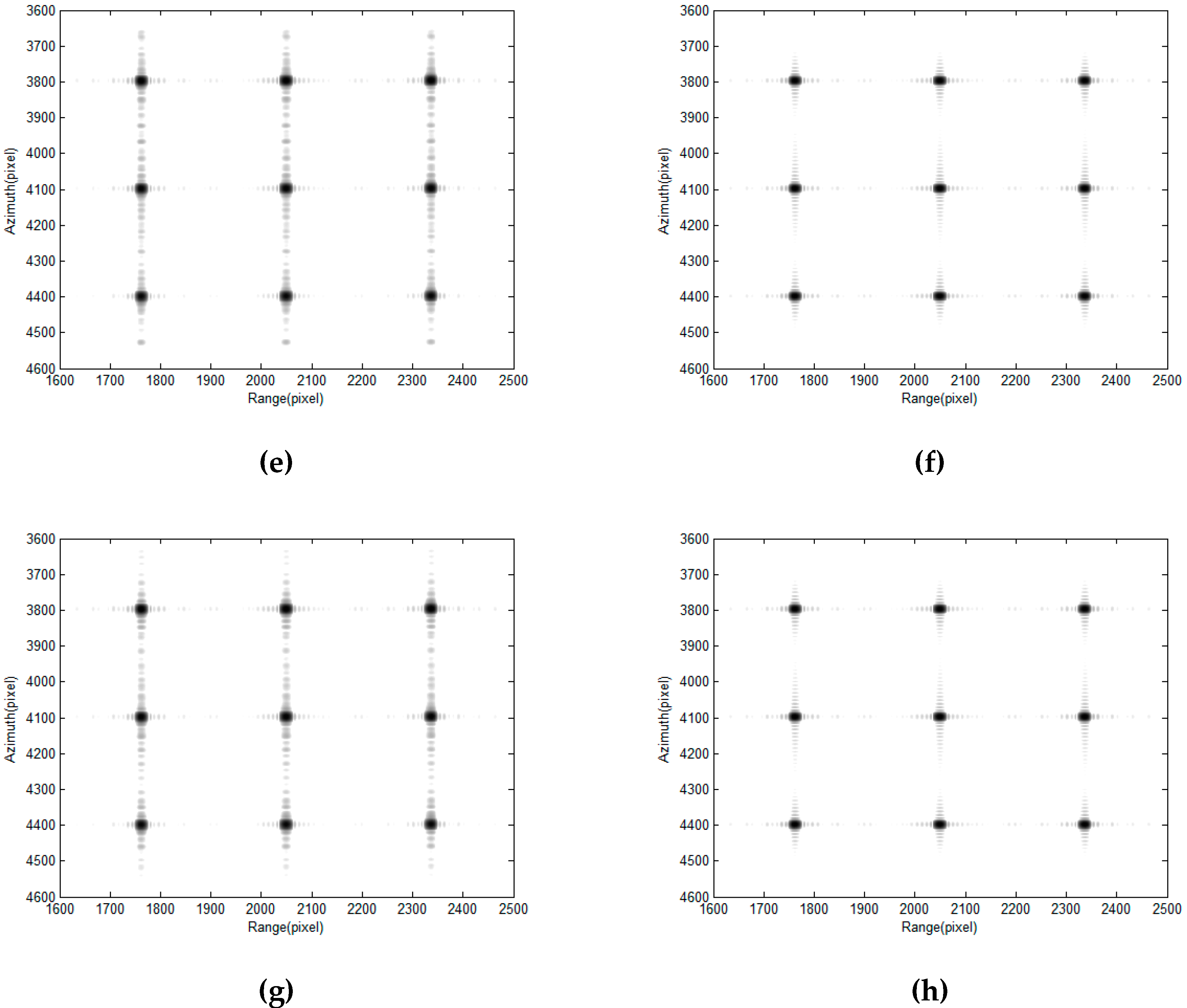
5. Simulation Result

A multi-channel SAR simulation was implemented using the parameters given in

Table 1. Simulation parameters.

Parameters	Value
Carrier frequency (fc)	10 GHz
Bandwidth (B)	200 MHz
Number of pulses (M)	1024 / 512
Range bins (Mr)	2048
Number of receive channel (N)	16
Element spacing	0.5 λ
Range resolution	1 m
Azimuth resolution	1 m
Velocity (vc)	150 m/s
Height of platform (Hc)	3000 m
SAR Squint angle (θ0)	15°
Range center	40 km
Jammer offset/ Direction of jammer(θJ)	35 km/ 10°
Jam noise ratio/Signal noise ratio	20 dB/ 15 dB

. The synthetic aperture time is about 4.4 s, and the number of received pulses is 1024. The range bin number used in simulation is less than that used in practice but sufficient to demonstrate the adaptive algorithm. At 40 km, the width of the SAR receiving beam is about 7° and the azimuth range of the SAR receiving beam is 5000 m.

The distribution maps of simulation points are given in Figure 4. The 3 × 3 individual scatters are distributed in this area, and the space between each scatter is 30 m. The jammer with noise interference was set to near the mainlobe direction of the antenna, 10 km away from the radar platform. The DOA of interference varied about 2° in the synthetic aperture time. The images were formed using a typical Range-Doppler algorithm for stripmap SAR.

The simulation results are illustrated in Figure 5. Figure 5a is the ideal image without any interference and Figure 5b is the image affected by interference, which clearly shows the large amount of degradation. Figure 5c,e,g show the image suppressed by conventional piecewise STAP processing where the numbers of sub-apertures are 16, 32 and 64, respectively.

It can be seen that the interference is effectively suppressed, but the azimuth focusing of the image is reduced to a certain extent compared with the original image, as the variation of adaptive weight vectors modulates the SAR waveform resulting in the image defocus. Figure 5d,f,h show the images suppressed by the piecewise constrained STAP method proposed in this paper. While effectively suppressing interference, the focusing performance is greatly improved. The processing result based on the piecewise constrained GSC algorithm is almost the same as the piecewise constrained STAP, which are not presented here. The target response characteristics are shown in Figure 6.

A Hamming window is used in the SAR process in order to reduce the sidelobe levels. It can be seen that the azimuth focusing performance of the conventional piecewise STAP processing is obviously degraded due to the destruction of the echo phase continuity between sub-apertures, and the sidelobes also increase to a certain extent. The result where the numbers of sub-apertures are 32 and 64 is similar to that in Figure 6. The specific quantitative analysis including peak side lobe ratio (PSLR), integral side lobe ratio (ISLR), and spatial resolution (3 dB width) of point targets are shown in

Table 2. Evaluation results of point targets simulation.

Theoretical Azimuth Resolution		1.19 m
Item	Number of Sub-Apertures	Conventional Method	Proposed Method
Simulation Azimuth Resolution	M = 16	1.48 m	1.27 m
	M = 32	1.49 m	1.27 m
	M = 64	1.47 m	1.27 m
Simulation Azimuth PSLR/ISLR	M = 16	−21.9 dB / −16.4 dB	−25.2 dB / −22.3 dB
	M = 32	−22.2 dB / −17.7 dB	−25.2 dB / −22.3 dB
	M = 64	−22.8 dB / −17.9 dB	−25.2 dB / −22.3 dB

.

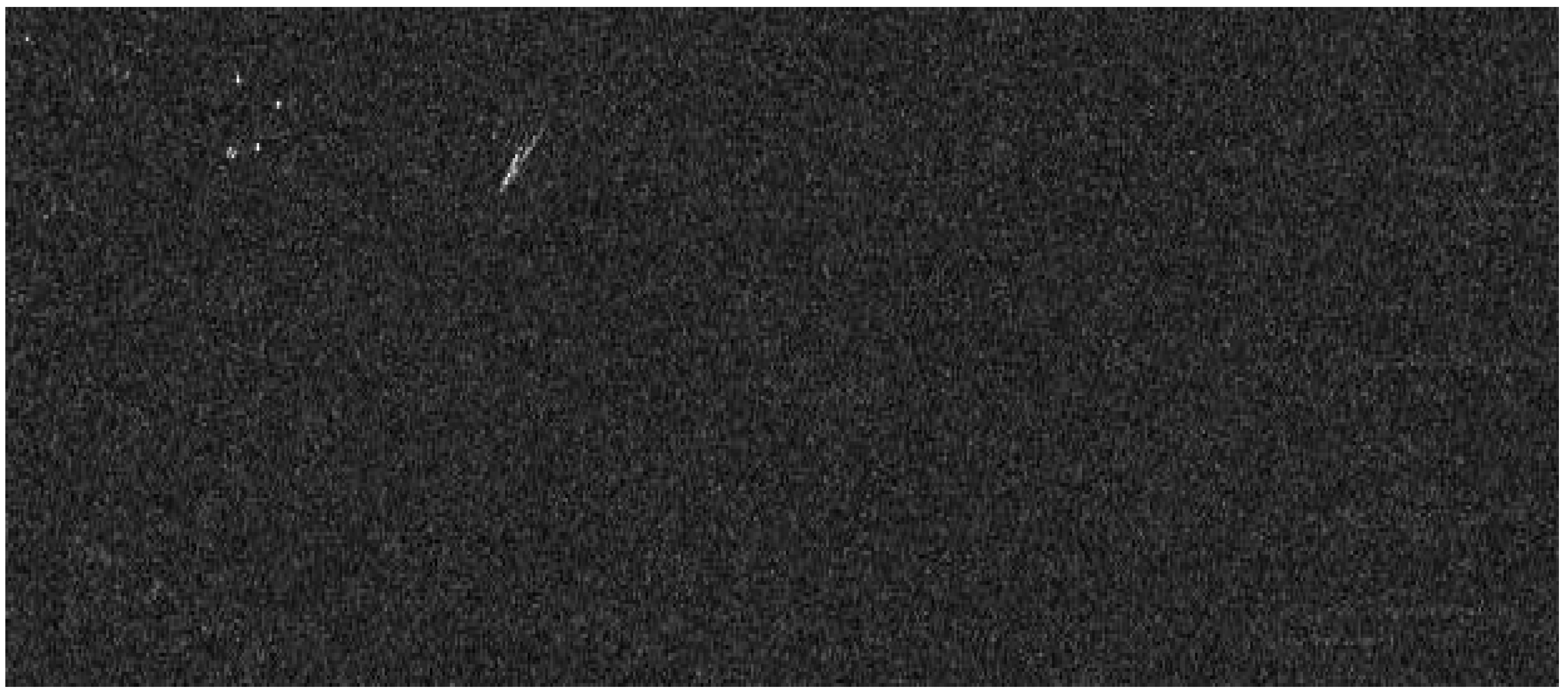
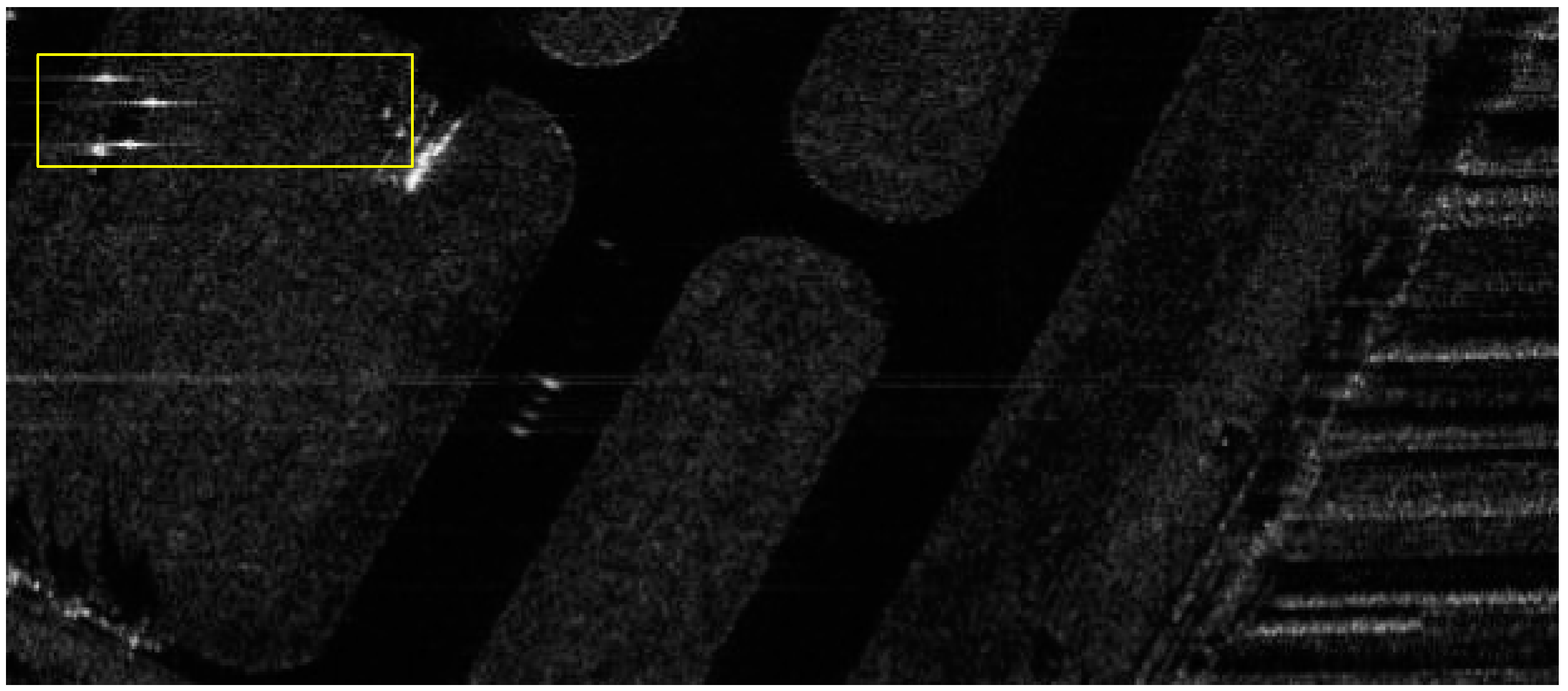
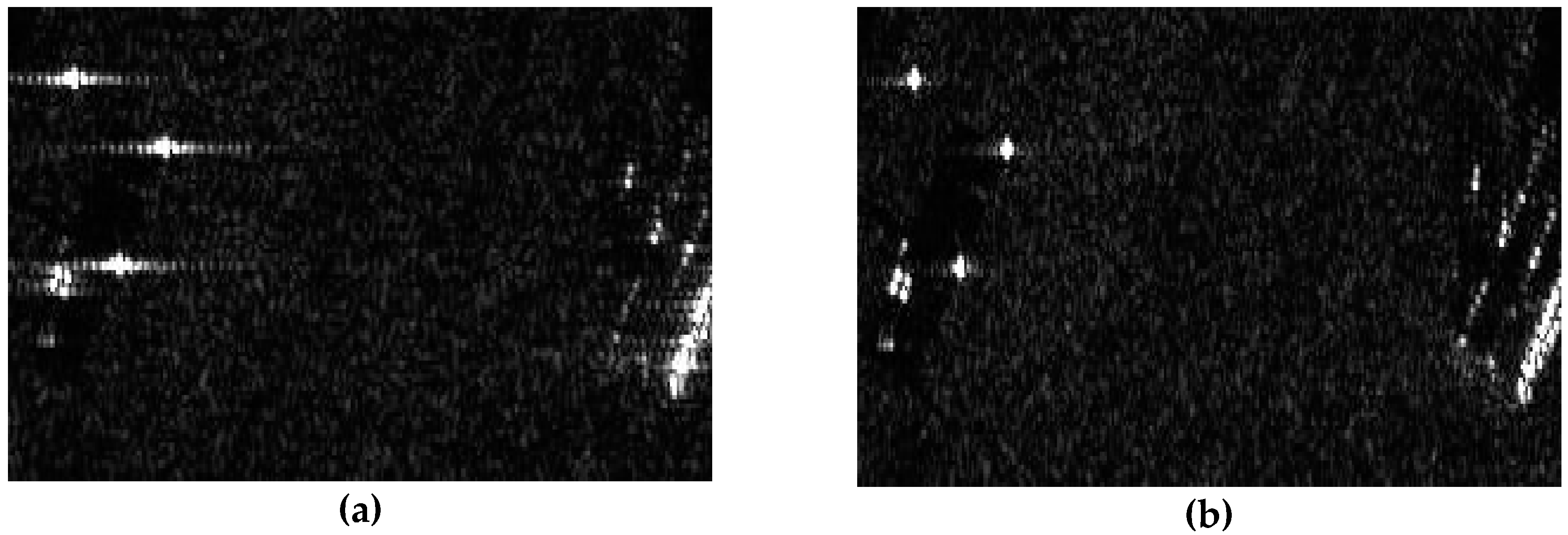
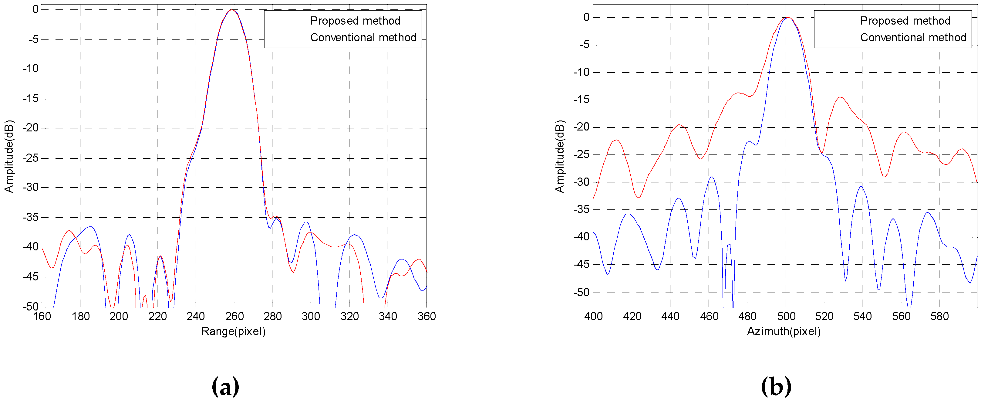
6. Measured Data Results

The algorithm is further validated by flight experiments. The data was collected by an X-band multi-channel airborne SAR whose bandwidth is 200 MHz and the theoretical resolution is 1 m × 1 m. The aircraft was flying along the southeast direction. The imaging area was located at 30 km, and the squint angle was about 15°. The jammer fixed near the imaging area was about 3° away from the main beam. The interference type transmitted by the jammer is wideband blanket jamming. The interference-to-noise (JNR) ratio in the original SAR image is more than 15 dB before interference cancellation. The total synthetic aperture time is 6.2 s, and the DOA of the interference varied about 2.5° during the period. Figure 7 is the SAR image before interference suppression and the ground echo was completely covered by the interference.

Figure 8 and Figure 9 are SAR images processed by conventional piecewise STAP and piecewise constrained STAP, respectively. It can be seen that the proposed algorithm can effectively suppress interference and improve azimuth focusing performance compared with the original algorithm.

In order to observe image quality improvement of the proposed algorithm more clearly, Figure 10 shows two local areas in the image. It can be seen that the proposed algorithm can significantly improve the focusing effect of the image.

Figure 11 shows the comparison of the point target profile, and the Hamming window is used in the SAR process in order to reduce the sidelobe levels.

To further evaluate the performance of the proposed algorithm, the measured parameters of PSLR, ISLR, and spatial resolution (3 dB width) of the corner reflector in the SAR image were calculated, and the results are listed in

Table 3. Evaluation results of point targets simulation.

Item	Conventional Method	Proposed Method
Azimuth Resolution	1.32 m	1.09 m
Azimuth PSLR/ISLR	−13.8 dB / −10.6 dB	−23.2 dB / −19.1 dB

. We can find that the performance parameters of the proposed algorithm are obviously superior to that of the conventional piecewise method.

7. Conclusions

Two improved STAP methods for SAR based on piecewise sub-apertures are proposed in this paper. In these methods, the entire synthetic aperture time is divided into several sub-apertures and the interference can be considered as stationary in each sub-aperture. The first algorithm is an element space STAP implementation, which is designed for interference cancellation and azimuth focusing in SAR by the piecewise data constraint. The second algorithm is the piecewise data constrained GSC, which is equivalent to the element space STAP approach if there is no signal mismatch. The proposed algorithms are validated through the model simulation and measured data to lay the foundation for further airborne applications.

References

1. Zhang, C. Synthetic Aperture Radar Principle, System Analysis and Application; Science Press: Beijing, China, 1989. [Google Scholar]
2. Liu, J.; Qiu, X.; Han, B.; Xiao, D. Study on geo-location of sliding spotlight mode of GF-3 satellite. In Proceedings of the 5th IEEE Asia-Pacific Conference on Synthetic Aperture Radar, APSAR, Singapore, 1–4 September 2015. [Google Scholar]
3. Mittermayer, J.; Lord, R.; Borner, E. Sliding spotlight SAR processing for TerraSAR-X using a new formulation of the extended chirp scaling algorithm. In Proceedings of the IGARSS 2003 Proceedings, Toulouse, France, 21–25 July 2003; pp. 1462–1464. [Google Scholar]
4. Dumper, K.; Cooper, P.S.; Wons, A.F. Spaceborne synthetic aperture radar and noise jamming. In Proceedings of the IEE Radar Systems, Edinburgh, UK, 14–16 October 1997; pp. 411–414. [Google Scholar]
5. Zhao, B.; Zhou, F.; Tao, M.; Zhang, Z. Improved method for synthetic aperture radar scattered wave deception jamming. IET Radar Sonar Navig. 2014, 9, 155–160. [Google Scholar] [CrossRef]
6. Wang, W.; Cai, J. A technique for jamming bi-and multistatic SAR systems. IEEE Geosci. Remote Sens. Lett. 2007, 4, 80–82. [Google Scholar] [CrossRef]
7. Li, W.; Liang, D.; Dong, Z. A new jamming method on parasitic spaceborne SAR system. In Proceedings of the IGARSS 2005 Proceedings, Seoul, Korea, 29 July 2005; pp. 4611–4614. [Google Scholar]
8. Smith, T.L.; Hill, R.D.; Hayward, S.D.; Yates, G. Filtering approaches for interference suppression in low frequency SAR. IEE Proc. Radar Sonar Navig. 2006, 153, 338–344. [Google Scholar] [CrossRef]
9. Miller, T.; Potter, L.; McCorkle, J. RFI suppression for ultra wide band radar. IEEE Trans. Aerosp. Electron. Syst. 1997, 33, 1142–1156. [Google Scholar] [CrossRef]
10. Zhou, F.; Xing, M.; Bai, X.; Sun, G. Narrow Band interference suppression for SAR based on complex empirical mode decomposition. IEEE Geosci. Remote Sens. Lett. 2009, 6, 423–427. [Google Scholar] [CrossRef]
11. Nguyen, L.; Tuan, T.; Wong, D.; Soumekh, M. Adaptive coherent suppression of multiple wide band width RFI sources in SAR. In Proceedings of the Algorithms for Synthetic Aperture Radar Imagery XI, Orlando, FL, USA, 12–15 April 2004; Volume 5427, pp. 1–16. [Google Scholar]
12. Lord, R.T.; Inggs, M.R. Efficient RFI suppression in SAR using LMS adaptive filter integrated with range/Doppler algorithm. Electron. Lett. 1999, 35, 629–630. [Google Scholar] [CrossRef]
13. Zhou, F.; Wu, R.; Xing, M.; Bao, Z. Eigen subspace based filtering with application in narrow band interference suppression for SAR. IEEE Geosci. Remote Sens. Lett. 2007, 4, 75–79. [Google Scholar] [CrossRef]
14. Zhou, F.; Tao, M. Research on Methods for Narrow-Band Interference Suppression in Synthetic Aperture Radar Data. IEEE J. Sel. Top. Appl. Earth Obs. Remote Sens. 2015, 8, 3476–3485. [Google Scholar] [CrossRef]
15. Rosenberg, L.; Gray, D.A. Constrained fast-time STAP techniques for interference suppression in multichannel SAR. IEEE Trans. Aerosp. Electron. Syst. 2013, 49, 1792–1805. [Google Scholar] [CrossRef]
16. Ender, J.H.G. Space-time adaptive processing for synthetic aperture radar. In Proceedings of the IEE Colloquium on Space-Time Adaptive Processing, London, UK, 6 April 1998; pp. 1–8. [Google Scholar]
17. Rosenberg, L.; Gray, D.A. Anti-jamming techniques for multichannel SAR imaging. IEE Proc.–Radar Sonar Navig. 2006, 153, 234–242. [Google Scholar] [CrossRef] [Green Version]
18. Guerci, J.R. Space-Time Adaptive Processing for Radar; Artech House: Norwood, MA, USA, 2003. [Google Scholar]
19. Titi, G.W.; Marshall, D.F. The ARPA/NAVY Mountaintop Program: Adaptive signal processing for airborne early warning radar. In Proceedings of the 1996 IEEE International Conference on Acoustics, Speech, and Signal Processing (ICASSP-96), Atlanta, GA, USA, 9 May 1996; pp. 1165–1168. [Google Scholar]
20. Bacci, A.; Martorella, M.; Gray, D.A.; Berizzi, F. Space-Doppler adaptive processing for radar imaging of moving targets masked by ground clutter. IET Radar Sonar Navig. 2015, 9, 712–726. [Google Scholar] [CrossRef]
21. Bacci, A.; Martorella, M.; Gray, D.A.; Gelli, S.; Berizzi, F. Virtual multichannel SAR for ground moving target imaging. IET Radar Sonar Navig. 2016, 10, 50–62. [Google Scholar] [CrossRef] [Green Version]
22. Su, H.; Liu, H.; Shui, P.; Bao, Z. Adaptive Beamforming for Nonstationary HF Interference Cancellation in Skywave Over-the-Horizon Radar. IEEE Trans. Aerosp. Electron. Syst. 2013, 49, 312–324. [Google Scholar] [CrossRef]
23. Fabrizio, G.A.; Gershman, A.B. Robust adaptive beamforming for HF surface wave over the horizon radar. IEEE Trans. Aerosp. Electron. Syst. 2004, 40, 510–525. [Google Scholar] [CrossRef]
24. Su, H. Adaptive HF interference cancellation for skywave over-the-horizon radar. Electron. Lett. 2011, 47, 50–52. [Google Scholar] [CrossRef]
25. Klemm, R. Space Time Adaptive Processing: Principles and Applications; IEE Press: London, UK, 1998. [Google Scholar]
26. Melvin, W.L. A STAP overview. IEEE Aerosp. Electron. Syst. Mag. 2004, 19, 19–35. [Google Scholar] [CrossRef]
27. Reed, S.; Mallett, J.D.; Brennan, L.E. Rapid Convergence Rate in Adaptive Arrays. IEEE Trans. Aerosp. Electron. Syst. 2004, 10, 853–863. [Google Scholar] [CrossRef]
28. Buckley, K.; Griffiths, L.J. An adaptive generalized sidelobe canceller with derivative constraints. IEEE Trans. Antennas Propag. 1986, 34, 311–319. [Google Scholar] [CrossRef]
Figure 1. Diagram of the multi-channel SAR. (a) 3D geometry model; (b) Geometry relationship in the slant plane.
Applsci 10 03609 g001
Figure 2. Processing diagram of the multi-channel SAR.
Applsci 10 03609 g002
Figure 3. Processing diagram of the generalized sidelobe canceller.
Applsci 10 03609 g003
Figure 4. Simulation point targets.
Applsci 10 03609 g004
Figure 5. Imaging simulation result. (a) Image with no interference; (b) Before interference cancellation; (c) Result of conventional STAP (M = 16); (d) Result of PC-STAP (M = 16); (e) Result of conventional STAP (M = 32); (f) Result of PC-STAP (M = 32); (g) Result of conventional STAP (M = 64); (h) Result of PC-STAP (M = 64).
Applsci 10 03609 g005aApplsci 10 03609 g005b
Figure 6. Comparison of point target profile (M = 16): (a) Range profile; (b) Azimuth profile.
Applsci 10 03609 g006
Figure 7. SAR image before interference suppression.
Applsci 10 03609 g007
Figure 8. SAR images processed by conventional piecewise STAP.
Applsci 10 03609 g008
Figure 9. SAR images processed by piecewise constrained STAP.
Applsci 10 03609 g009
Figure 10. Detailed results of a local area: (a) Result of conventional STAP (M = 16); (b) Result of PC-STAP (M = 16).
Applsci 10 03609 g010
Figure 11. Comparison of the point target profile (M = 16): (a) Range profile; (b) Azimuth profile.
Applsci 10 03609 g011