Testing the Accuracy of the Calculation of Gold Leaf Thickness by MC Simulations and MA-XRF Scanning

Featured Application

Characterization of surfaces in multilayered structures is a requirement in many application areas. Such characterization should be nondestructive, and, in some cases, it must be performed in situ. This is the case of precious Cultural Heritage samples. The use of X-ray fluorescence analysis is currently one of the few solutions. When a large surface must be characterized, a MA-XRF scanning system can also be employed.

Abstract

The use of X-ray fluorescence (XRF) scanning systems has become a common practice in many application sectors. In multistratified and heterogeneous samples, the simple analysis of an XRF spectrum as a response of the entire sample is not reliable, so different spectral analysis techniques have been proposed to detect the presence of surface stratification. One commonly studied case is that of gilding, i.e., the presence of a superimposing gold-leaf layer. The observation of changes in the net peak ratios of a single element or of several elements in an XRF spectrum is a well-developed practice, but is still not used in the case of XRF scanning (macro-X-Ray fluorescence scanning, MA-XRF), a technique that can be described as the extrapolation of XRF spot analysis to a second dimension, scanning a sample surface instead. This practice can yield information on the overlaying layer thickness, if some properties of the sample are known—or estimated—beforehand, e.g., the overlapping layer’s chemical composition and the matrix effect contribution from the bulk material (thick ratio). This work proposes the use of an algorithm to calculate the thickness distribution of a superimposing gold layer accurately and automatically through the differential attenuation method by using MA-XRF datasets in a total noninvasive manner. This approach has the clear advantage over the traditional spot sampling of allowing the generation of a surface heightmap to better visualize and interpret the data, as well as a considerably larger sample space. Monte Carlo simulations were used to verify the influence of the medium used to adhere the gold leaves to the substrate and to generate known spectra to assess the algorithm’s accuracy.

1. Introduction

The use of metal coatings on surfaces is a very common practice in different technological sectors with the aim of either protecting the surface or to achieve specific material properties, such as in electronics, photonics, and biomaterials [1]. The determination of gold leaf thickness for heritage purposes is a practice that has been performed for decades [2]. The information yielded by such investigations can give further insight into the technology, manufacturing techniques, and binding mechanisms between the gold leaf and the artwork it was applied to [3,4]—be it panel paintings, canvases, gilded metals, or frescoes [2,5]. When establishing restoration protocols, this information is of great value, so the artwork can be restored to as close as possible to its original state. Moreover, technological traits of the manufacturing techniques of gold leaves can serve as anchors for the establishment of chronologies and different workshops.

Customarily, the determination of gold leaf thickness is performed by microsampling and cross-section analysis, a microdestructive approach that is not always feasible (or desired) when dealing with objects of cultural heritage [6,7]. An alternative to microsampling is the use of the differential attenuation of fluorescence radiation [8], basing on the concatenation effects of (a) the production of photons in the sample’s substrate and (b) their subsequent attenuation by the gilding’s uppermost layer. This approach has been previously applied to a series of objects of cultural heritage [9,10,11,12]. Nevertheless, archaeological materials and works of art are known to be considerably heterogeneous, i.e., the substrate underneath the gold foil can differ throughout the sample, so the study of only one or few points on the surface may yield biased information [8,13].

Furthermore, different mordants used to adhere the gold foils or leaves to the substrate surface and protective layers further applied to the finished gilded surface can enhance the attenuation effects. Nardes et al. [9], when investigating gold foils protected with mica, demonstrated that the addition of a protective layer can introduce considerable errors to the estimated mean thickness by the different attenuation method.

Macro-X-ray fluorescence scanning (MA-XRF) is a nondestructive and widespread technique in the field of heritage science, which provides a large set of spectra and can generate elemental distribution maps [14,15,16,17]. Using its dataset for applying the differential attenuation method is an obvious approach to improve sampling space and verify the existence of substrate inhomogeneities, avoiding biases, and obtaining a more accurate mean gilding thickness value. Unfortunately, the evaluation and manual inspection of each spectrum for a precise determination of the net peak areas is a time consuming operation; therefore, the development of an automated algorithm for processing the large data provided by MA-XRF scans, giving each spectrum net peak ratios, is required [18].

In this study, to determine the influence of a binding interface and apply the differential attenuation method to MA-XRF datasets representing gilded artworks (paintings), an algorithm was developed to automatically extract the net peak areas, generate the elemental distribution maps, and to automatically calculate the overlapping layer thickness at each sampled point. The dataset used was obtained by scanning one gilded sample with known parameters crafted to test the capabilities and limitations of the proposed methodology and algorithm. Monte Carlo simulations were performed to generate known spectra and test the outputs of the algorithm as well as to assess the influence of an intermediate resin layer between the gold leaf and the substrate and the continuum contribution.

2. Materials and Methods

In order to test the proposed methodology as a noninvasive and more accurate determination method of gold leaf mean thickness, a sample with known parameters was prepared. Monte Carlo simulations, representing analytical volumes of interest sufficiently similar to the sample, were performed with the X-ray Monte Carlo (XRMC) package [19]. The sample was analyzed by MA-XRF scanning, and the dataset generated was used to automatically calculate the mean gilding thickness. To obtain the most representative data, the thickness calculations were performed over specific areas of interest (AoI), avoiding matrix composition inhomogeneities that are visible in the elemental distribution maps. The matrix thick ratio was obtained by directly measuring the substrate (regions A and D).

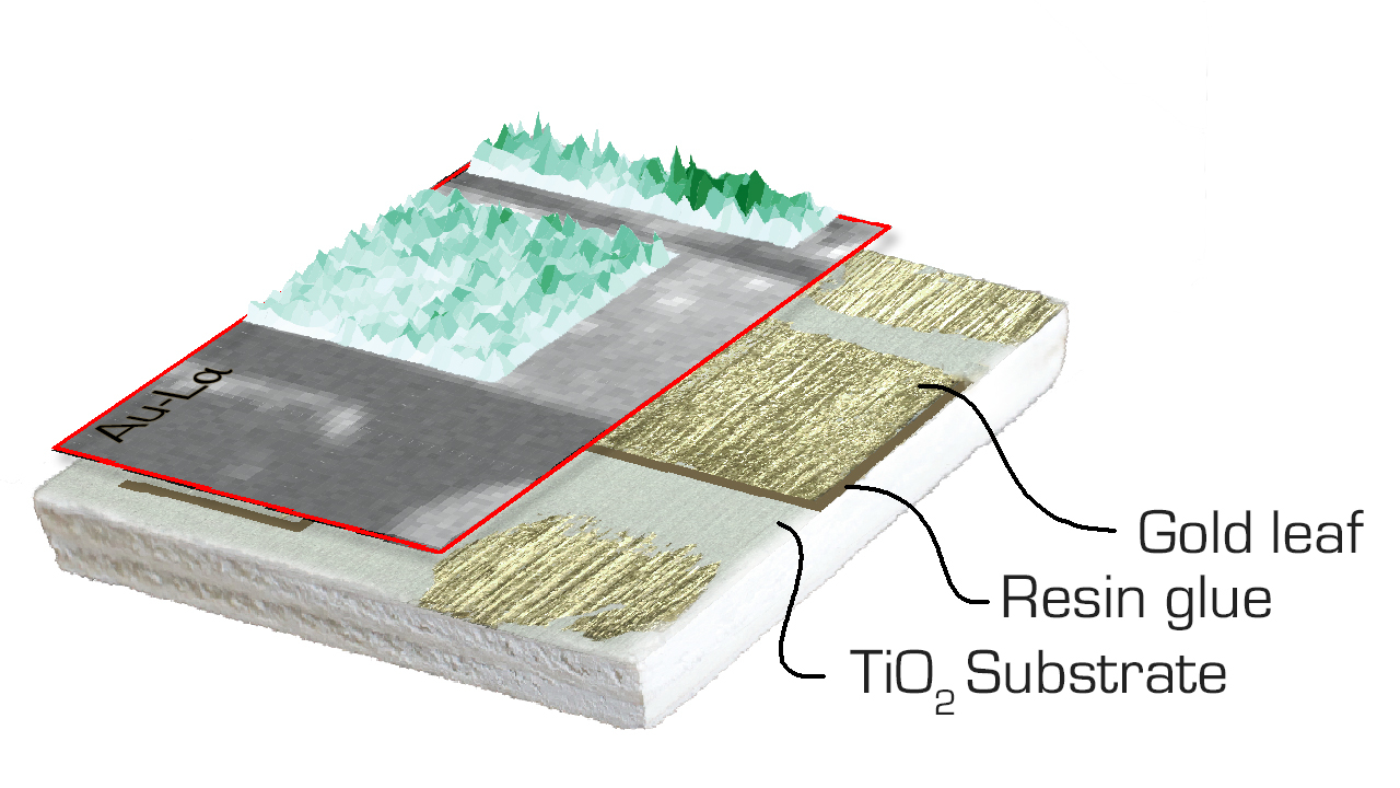
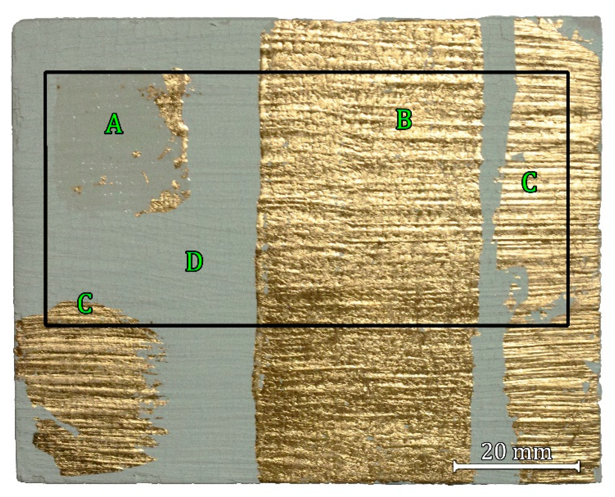
2.1. Sample Preparation

The sample prepared can be seen in Figure 1 below. The base, a plywood piece of 91 × 72 mm², was polished with 250 grit sandpaper. The plywood was then covered with several layers of titanium dioxide substrate to create a sufficiently thick layer and assure it can be considered infinitely thick (>150 μm). This means that all X-ray photons from the beam interact inside the sample, thus allowing a better estimation of the gold leaf thickness. In real cases, it is also common to find lead- or zinc-based preparation layers, especially in historical artworks [20]. Titanium white is a well-known pigment widely used in contemporary artworks, and it was chosen due to its accessibility (TiO₂ powder can be readily found) and nontoxicity when compared to lead. Moreover, Ti-K lines are well separated from Au-L lines, differently from zinc K-lines. In this way, titanium is the ideal candidate for the proposed experiments’ substrate.

The preparation layer (substrate) was made by mixing roughly 10 parts of TiO₂ powder (produced by Abralux Colori Beghè s.r.l, Costelmare (CO), Italy) with seven parts of water and one part of vinyl-based glue (deSmovil 72 – produced by Italchimici s.r.l, Trevi (PG), Italy) and was left to dry for 24 h. Afterwards, one thin layer of gilding glue (“missione per oro in fogli” – produced by Primo Pennesi e F.lli s.o.s, Rome (RM), Italy) was applied over regions A and B (Figure 1). When the glue was sufficiently dry, the gold leaves provided by CTS Europe^®, with an approximate thickness ranging from 0.15 to 0.25 μm, were applied on top of it. The leaves are 98.5% pure with no specifications on the impurities. Other pieces of gold leaves were applied to region C by wetting the substrate with a soft brush and then sticking the leaves directly to it, devoid of any gilding glue. The small leaf fragments, evident in the right portion of the area of interest (AoI) A, are a product of the lack of the craftsman expertise in gilding, resulting in the accidental deposition of leaf fragments in that portion during the gilding process. Nonetheless, the central and upper left regions of AoI A are devoid of gold and still usable for its purpose.

2.2. Monte Carlo Simulations

XRF spectra simulations were performed with a modified version of the XRMC package, version 6.4.1., a Monte Carlo algorithm based on the xraylib database [21]. In this custom version, it is possible to simulate rough surfaces as well [22]. This package is capable of simulating interactions up to any order. For the present work, a threshold was set at the third order, since, as the order increases, errors in the atomic parameters used in the interaction’s simulation are accumulated. Therefore, for higher interaction orders, the simulated value loses its significance. This code can simulate several types of fluorescence lines, including M-lines, also allowing the simulation of more complex sample geometries, surface roughness, and the characterization of both structure and elemental composition within a multilayered structure [19,22,23].

Regions A, B, C, and D depicted in Figure 1 were simulated. For the present simulations, all irradiated volumes were simulated as a stack of parallel planes. For the A region, a bilayered volume was considered, with a 0.5 cm thick TiO₂ substrate and a 50 μm thick resin layer (11 wt% H, 11 wt% O and 78 wt% C). The substrate thickness is enough to assure this layer behaves as an infinitely thick layer. It is well-known that above the infinitely thick threshold, the exceeding thickness can be disregarded as it does not affect the outputs.

Region B was simulated analogously to region A with the addition of an uppermost 0.20 μm thick 98.5% gold 1.5% Ag layer. Region C was simulated as a bilayered structure with a 0.5 cm thick TiO₂ substrate and a 0.20 μm thick 98.5% gold 1.5% Ag layer. Lastly, region D was simulated as a monolayered structure composed solely by a 0.5 cm thick TiO₂ substrate. The simulated resin thickness was exaggerated (50 μm) to clearly highlight any influence caused by it. The gold layer thickness was chosen as an average of the leaves used in the real sample. Both measured and simulated data were analyzed in an analogous way.

The excitation tube profile used in the simulations was of an Ag-anode tube, while the system geometry was the same as the physical analytical system, 27° between tube and the sample normal. The tube and detector were positioned symmetrically.

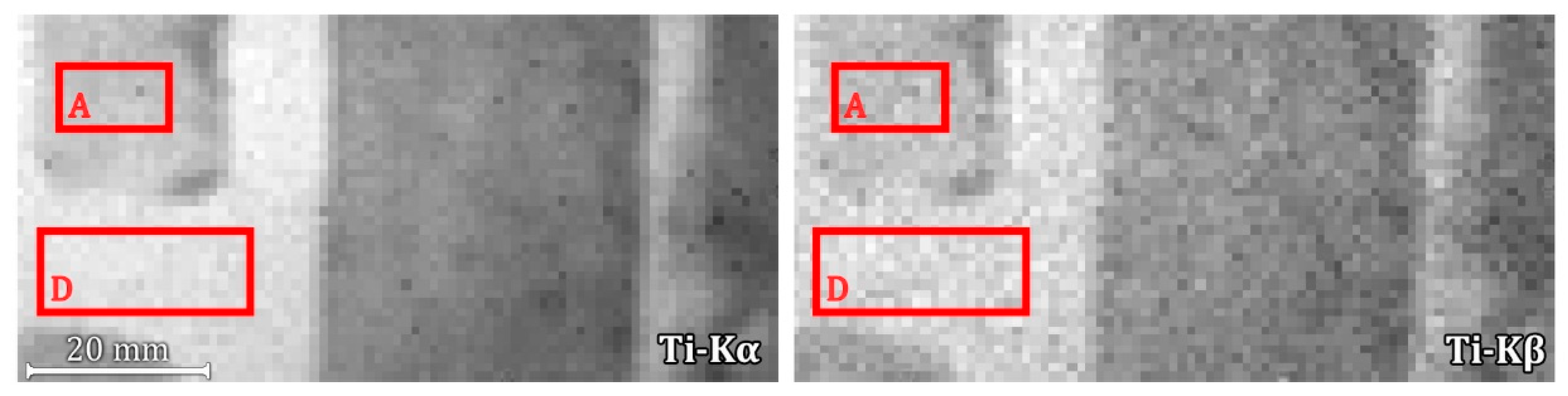
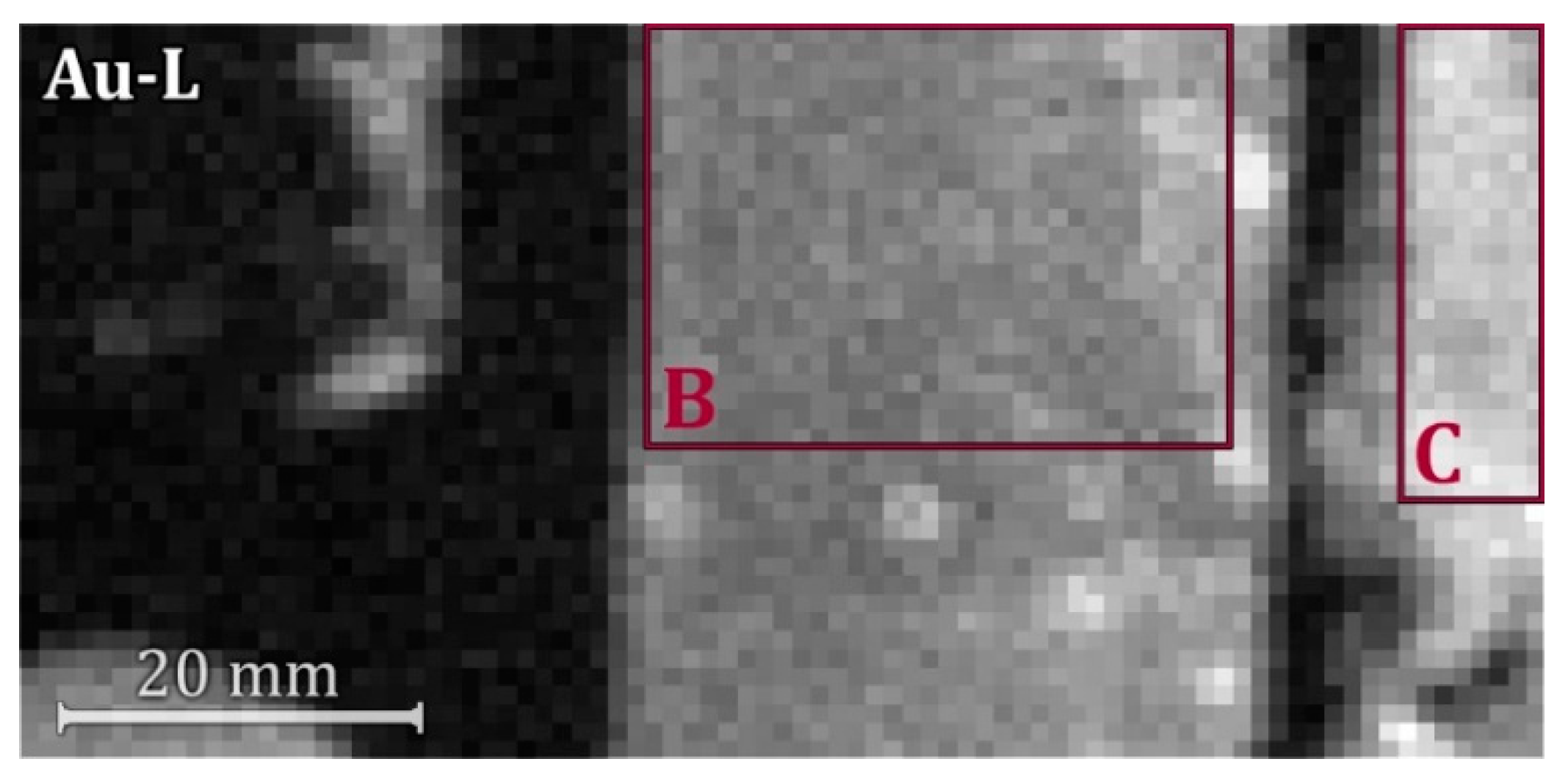
2.3. MA-XRF Scanning

The MA-XRF scanning was performed with a portable prototype scanning system built in a collaboration between the Istituto Nazionale di Fisica Nucleare (INFN)—Roma TRE and a private company, Ars Mensurae. The system features an exchangeable and modular scanning head and different x–y scanning stages. The head components used for the present analysis were: one low-power (4W) Moxtek^® Ta-target tube (collimated to 1 mm) and one AMPTEK^® 123SDD detector having an active area of 25 mm² and a thickness of 500 μm. The energy resolution is of 125 eV @ the Mn-K_α line (5.9 KeV). The scanning stage used was the smaller, portable version, capable of holding samples up to 200 × 200 mm² in dimension [17]. The total scanned area was 83 × 40 mm² (Figure 1) and the dwell-time was 3 s. Tube voltage and current were set to 35 KV and 17 μA, respectively.

3. Thickness Determination

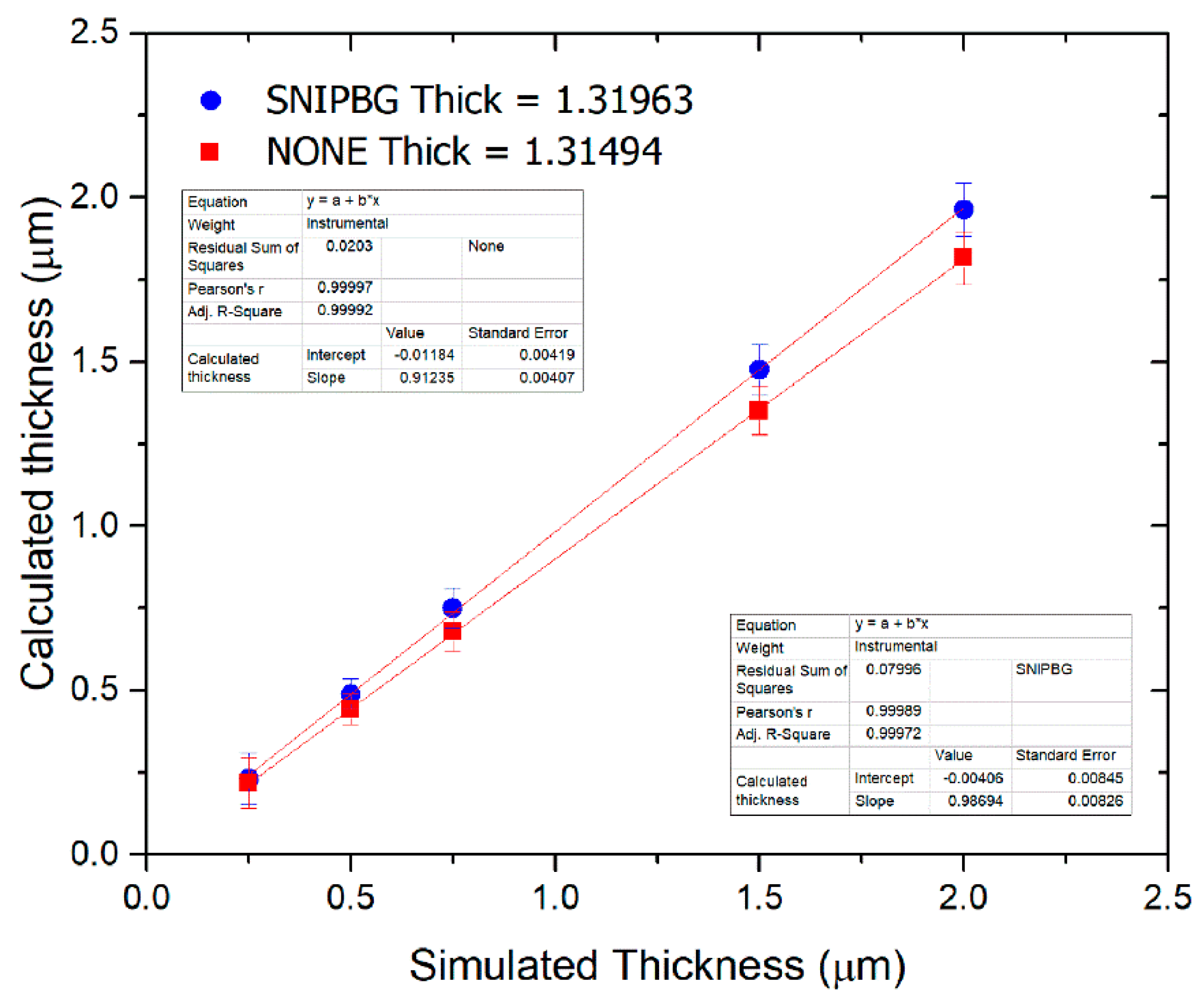
3.1. Peak Area Calculation

A precise determination of the net area of peaks of interest is fundamental for an accurate thickness estimation through the differential attenuation method [8]. To achieve such precision, XRF spectra are usually manually inspected. This approach is feasible when analysing few or dozens of spectra, but impracticable when dealing with MA-XRF datasets composed of at least thousands of spectra. To overcome this problem, an algorithm was proposed to automatically determine the net peak areas of interest.

The spectrum evaluation is performed in three steps: (a) calculate the full-width at half maximum (FWHM) for a gaussian centred at the theoretical peak position, (b) search for a peak maximum in a 2*FWHM window, verify if it matches with the theoretical centre, and (c) check the signal-to-noise ratio (SNR) criteria. If the peak maximum is slightly offset due to calibration issues, the FWHM window is recentred. The theoretical values used for centring and locating the peaks are obtained from the xraylib package [20]. Background contribution is calculated following the Statistical Non-Linear Iterative Peak Clipping (SNIPBG) method [24] and the parameters are set by evaluating randomly sampled spectrum instead of a derived spectrum.

Since MA-XRF spectra usually present low statistics, the net area is calculated over the raw data. No fitting is performed to save on computational time. Therefore, the proposed method requires that the peaks of interest be well separated and defined, as no deconvolution method is yet implemented.

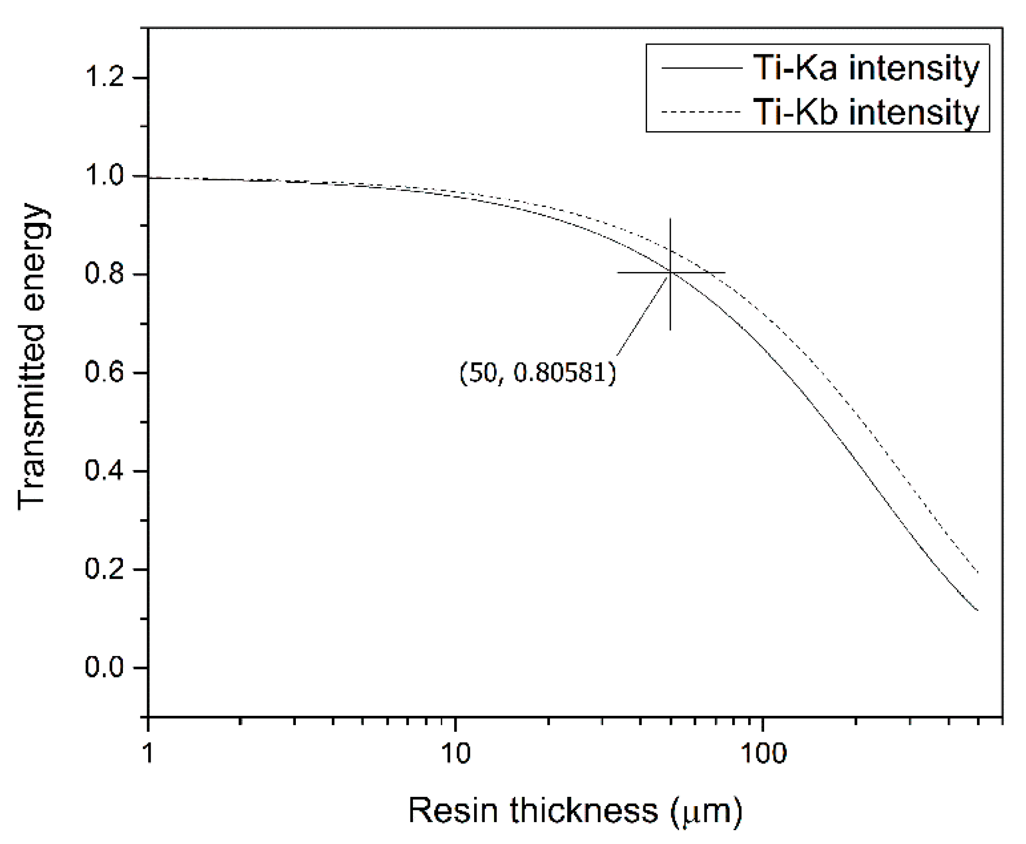
3.2. Differential Attenuation

The excited atoms of each element emit X-ray photons at different energies that can be synthetically categorized into the so called K_α and K_β or L_α, L_β and L_γ lines when K and L shells are involved. When a sample is said to be infinitely thin, i.e., when secondary interactions are negligible, the ratio between these lines for a single element can be calculated and are tabulated [25]. When considering secondary interactions and matrix effects, the ratio between the emission lines changes exponentially with increasing material thickness until reaching a plateau; from this point onwards, the sample can be considered infinitely thick. If the element is in a mixture, the thick ratio can still be calculated, but the weight percentage of each present element must be known. An alternative method is to directly measure the intensity ratios from an XRF spectrum taken from the exposed substrate which applies for samples for which the exact composition cannot be fully constrained.

If the emitted X-rays from the sample’s substrate traverse a superimposing layer, they will be attenuated proportionally to their energy and the superimposing layer’s thickness and composition. In this way, by comparing the ratio between two distinct lines before and after attenuation, one can estimate the thickness of the traversed superimposing layer. The differential attenuation theoretical background has been extensively discussed elsewhere [8,12,18,26].

In the present work, the ratios between Ti-K_α and Ti-K_β were evaluated. Figure 2 shows the areas sampled for measuring the thick ratio. For the direct substrate, it was measured as an average mean of several spots from Region D and from one spectrum taken with a longer acquisition time (30 s). The mean value obtained was 5.31 and that from the single spectrum was 5.32. When measuring the substrate with resin (AoI A) the mean value was slightly lower: 5.20.

The gold leaf thickness at each point was calculated following Equation (1) [9,18]:

$$d=\frac{sin\Psi }{-{\mu }_L\left(E_{K_{\alpha }}\right)+{\mu }_L\left(E_{K_{\beta }}\right)}ln\left[\frac{\left(I_{K_{\alpha }}/I_{K_{\beta }}\right)}{{\left(I_{K_{\alpha }}/I_{K_{\beta }}\right)}_{thick}}\right]$$

(1)

where Ψ is the X-ray tube and detector angle with the sample surface, μ_L is surface layer linear attenuation coefficient, $\left(I_{K_{\alpha }}/I_{K_{\beta }}\right)$ is the Ti K_α/K_β ratio recorded at the pixel and $\left(I_{K_{\alpha }}/I_{K_{\beta }}\right){}_{thick}$ is the corresponding thick ratio.

The statistical error on the measured Ti K_α/K_β ratio is:

$$\Delta \mathrm{R}=\frac{R}{\sqrt{I_{K_{\alpha }}}}\sqrt{1+R}$$

(2)

where R = $\left(\raisebox{1ex}{$I_{K_{\alpha }}$}\!\left/ \!\raisebox{-1ex}{$I_{K_{\beta }}$}\right.\right)$.

Therefore, the resolving power and error can be calculated through Equations (3) and (4) below:

$$\Delta d=\frac{\sqrt{1+R}}{\sqrt{I_{K_{\alpha }}}}\frac{sin\Psi }{-{\mu }_L\left(E_{K_{\alpha }}\right)+{\mu }_L\left(E_{K_{\beta }}\right)}$$

(3)

$${\sigma }_{AoI}=\sqrt{{\sigma }_{stat}^2+{\sigma }_{samp}^2+{\sigma }_{inst}^2}$$

(4)

where, in Equation (4), subindexes stat, samp, and inst correspond to the statistical, sample, and instrumentation variances, respectively. The latter is the variance sum of geometrical factors and calibration (matrix thick ratio) uncertainties.

4. Results and Discussion

Figure 3 shows the AoIs where thickness calculations were performed. Brighter spots present in the outbounds of AoI B are probably due to manufacturing defects and indicate a more intense signal of gold where attenuation effects are probably higher. For this reason, brighter spots were avoided. Area of Interest C was selected from the sample’s region C rightmost portion (Figure 1). Manufacturing defects are clearly present in the lower-right part and were left outside. A total of 3320 spectra were evaluated to calculate the net peak areas and generate the elemental distribution maps. For the thickness calculation over the whole gilded area, 1368 spectra were considered; for AoIs B and C, 965 spectra were considered.

The simulated spectra obtained from MC simulations were analyzed, and the mean thickness value obtained disregarding the resin layer (volume simulating region C) was 0.19 ± 0.01 μm, demonstrating that the proposed algorithm and methodology is accurate and precise when evaluating the simulated spectra. High precision was expected when evaluating the simulated spectra, as the linear attenuation parameters for Equation (1) could be exactly set. When evaluating the simulated spectra representing region B, where a 50 μm thick resin layer is present as an adhesive intermediate layer, the obtained gold leaf thickness is almost doubled: 0.35 ± 0.01 μm. This may be due to the logarithmic nature of Equation (1), where small changes in the measured peak ratio cause large changes in the calculated thickness value, highlighting the need for a proper calculation or measurement of the substrate thick ratio. For the calculations, the parameters of Equation (1) remained unchanged, since the linear attenuation factors considered are solely those of the layer whose thickness is being estimated (i.e., the gold layer) and the thick ratio is that of the substrate. Therefore, any further attenuation titanium lines have undergone, caused by the resin layer, could not be accounted and systematic errors were introduced, exaggerated by the logarithmic function. A workaround has been proposed by Nardes et al. [9], modifying Equation (1) to account for additional attenuation effects caused by a coating layer. In Figure 4, a significant decrease in the Ti-K-lines signal intensity can already be appreciated while traversing a 10 μm thick resin layer. At 50 μm thickness, about 20% of the Ti-K_α signal is absorbed by the layer.

The calculated average thickness distribution obtained for AoI B and C are given in

Table 1. Average golf leaf thickness calculated over AoIs B (with resin) and C (without resin).

	Average Gilding Thickness (μm)
Sample	With Resin		Without Resin
	Mean	Std. deviation	Mean	Std. deviation
Simulated Sample	0.35 μm	0.01 μm	0.19 μm	0.01 μm
Real Sample*	0.16 μm	0.09 μm	0.23 μm	0.13 μm

⁺ AoI B contains 715 sampled spectra; ^* AoI C contains 250 sampled spectra.

. Different from what was observed in the simulated spectra, there is no significant or immediately observable difference between the values (considering the standard deviation). This may be due to the statistics of the MA-XRF dataset, presenting a higher number of samples, and spectra with lower count statistics compared to traditional XRF spot analysis. Firstly, it must be noticed that the effective thickness of the resin applied to the substrate after drying can be considerably smaller than the 50 μm used in the simulations, as previously mentioned. Secondly, the simulated resin layer is considered as a dense and homogeneous layer, disregarding the existence of pores or air between resin and gold leaf, which can result in a further increase in the attenuation effects compared to what is experimentally observed. The effects of a thinner resin layer and the presence of air (considering the sample was not burnished) are competitive; a thinner layer results in less observable effects in the final results as the presence of air reduces the layer (in this case resin + gold leaf) linear attenuation coefficients, resulting in a slightly overestimated result.

The influence exerted by the background contribution over the calculated mean thickness was also tested with Monte Carlo simulated spectra. Figure 5 shows a linear fitting comparison between values obtained using the SNIPBG method and without considering any background contribution. Different gold leaf thicknesses were simulated, from 0.25 μm up to 2.0 μm, on top of a pure lead substrate. Lead L-lines present a considerably higher signal-to-noise ratio that can better highlight the background contribution effects. It must be observed that the simulation setup used to account for background contributions does not represent the experimental setup. Its purpose was to emphasize any contributions, if present, and point out if corrections must be made and when.

It can be observed that in the lower end, for very thin leaves, the background contribution does not significantly impact the results. As the overlapping layer thickness increases, discrepancies start to appear, and a background estimation method is required to achieve the best results.

To assess if any difference would be noticed in the experimental data (acquired with a Ta-target tube), and because the simulated data (Figure 5) was obtained using a different, Ag-target tube profile, the prepared sample was also evaluated without background subtraction. This factor can be crucial when verifying the influence of background effects on the thickness calculations, as different tubes will present different emission spectra. In any case, the mean thickness values were not significantly impacted. AoI B + AoI C mean thickness, considering the background contribution, was 0.18 ± 0.10 μm vs. 0.17 ± 0.10 μm without it. Moreover, the relatively low counts of the present MA-XRF dataset are not enough to create an appreciable continuum which, in this case, can be disregarded.

A 3D-heightmap of the thickness values calculated for AoIs B and C is shown in Figure 6. A concentration of slightly higher values is observed in the rightmost part of AoI C.

The grouped bins histograms of AoI B and C are shown in Figure 7. The distributions shown in the histograms exhibit an asymmetric shape (with skewness values 0.51 and 0.85, respectively) and a deviation from a normal distribution is evident for AoI C (kurtosis 1.1). As for AoI B, it can be observed that the calculated thicknesses are slightly inaccurate (more than 50% of the calculated thicknesses are lower than 0.15 μm). However, it is useful to underline that the means in Table 1 are calculated from histograms and, therefore, can be affected by the distribution shape as underlined above. The inaccurate results may be, in a first approach, attributed to the presence of resin, which presents significantly different physical properties compared to the gold leaves, introducing several outliers to the distribution, and changing the histograms’ appearance (truncated distribution). The resin presence is not accounted for by the measuring system (Equation (1)), and, as previously discussed, will introduce systematic under- or overestimations.

Therefore, the overall average calculated in AoI B region (0.16 μm) is probably a systematic underestimation of the true thickness, which can be due to many factors, such as the presence of a resin adhesive (in the resin-less region the calculated mean thickness is 0.23 μm) or, on a second approach, simply due to roughness effects (not taken into consideration). For the latter, variations in the impinging radiation and output angles change the absolute path travelled by the X-ray beam and fluorescence lines, respectively. This variation, even small, can introduce errors in the $\left[\left(I_{K_{\alpha }}/I_{K_{\beta }}\right)/{\left(I_{K_{\alpha }}/I_{K_{\beta }}\right)}_{thick}\right]$ factor that are emphasized by the logarithmic function in Equation (1), which, compared to the considerably small value being evaluated, may appear considerably high.

In addition, the histogram shown as the possible distribution is a truncated one, which can be presumed because all the values are calculated normalizing the peaks ratio to an estimated value $\left(I_{K_{\alpha }}/I_{K_{\beta }}\right){}_{thick}$. Area of interest C, devoid of resin, presented better results with a relatively symmetric histogram with a large right tail. The tailing may be due to the concentration of greater thickness values observed at the rightmost portion of AoI C (Figure 6), which in turn may have resulted from fabrication defects present in the substrate (lower Ti signal and darker region in the rightmost part—Figure 2). The presence of resin disturbs the results, causing a systematic error. Furthermore, when recalculating the mean thickness for AoI B considering a thick ratio, $\left(I_{K_{\alpha }}/I_{K_{\beta }}\right){}_{thick}$ term in Equation (1), sampled from region A (Figure 2), the mean value decreases only slightly.

The calculated statistical error in the thickness determination is about 0.07 μm (Equation (3)). Therefore, what we observe in the measured thicknesses in both AoI B and C is mostly statistical fluctuation of data. However, the observed mean thickness shift (Table 1), which is less than the standard deviation, is still valid. It is worth noting that the 0.07 μm shift, exactly the same as the statistical error, would be hardly measured with traditional spot sampling, but due to the large amount of data from MA-XRF scanning, it can be detected, as shown by the results.

5. Conclusions

The measurement of gilding thickness has become a very common practice, and in this paper, the possible advantages of using a MA-XRF scanner for thickness testing have been analysed in more detail. Apart from allowing the detection of inhomogeneities in the sample surface to a limited extent, avoiding areas that can introduce errors, the MA-XRF dataset provided a larger sample space to enhance the statistical power. The statistical error calculated with the present dataset for estimating a mean gilding thickness is about 0.07 μm (Equation (3)). As shown in Table 1, the observed standard deviation of AoI B is 0.13 μm, which, being the same as the calculated statistical error of thickness determination (Equation (2)), leads to a spread of data due to possible changes in σ²_samp of 0.11 μm (Equation (4)). Therefore, it is reasonable that the result is coherent with the possible thicknesse variation given by the gold leaf manufacturer.

The present results show how the thickness measurement from a large dataset with a spatial average over a gilded area is possible and has advantages, such as the possibility of detecting the presence of an adhesive nonabsorbing layer used for gilding, with certain limitations. Nonetheless, further studies with different types of mordants are still needed. A careful examination of the histograms (Figure 7) shows that the presence of the resin layer can be inferred from the shift of the average value downwards, but also from the evident modification of the structure of the histogram. The latter fact is supported by the extreme sensitivity that was observed in the MC simulation with the presence of an adhesive resin (shifting the thickness average upwards). Overall, a noninvasive and indirect estimation of gold leaf thickness applied to a homogeneous or inhomogeneous substrate is demonstrated to be possible with the proposed methodology, with some restrictions. In this case study, a titanium dioxide substrate was used and tested. Further studies are required to test the proposed methodology with different substrates, e.g., lead white, extending the method’s applicability to older artworks prior to the mass production of titanium dioxide (ca. 1916).

References

1. Giurlani, W.; Berretti, E.; Innocenti, M.; Lavacchi, A. Coating Thickness Determination Using X-ray Fluorescence Spectroscopy: Monte Carlo Simulations as an Alternative to the Use of Standards. Coatings 2019, 9, 79. [Google Scholar] [CrossRef] [Green Version]
2. Cesareo, R. Non-destructive EDXRF-analysis of the golden haloes of Giotto’s frescos in the Chapel of the Scrovegni in Padua. Nucl. Instrum. Methods Phys. Res. B 2003, 211, 133–137. [Google Scholar] [CrossRef]
3. Ridolfi, S. Gilded copper studied by non-destructive energy-dispersive X-ray fluorescence. Insight Non-Destr. Test. Cond. Monit. 2018, 60, 37–41. [Google Scholar] [CrossRef]
4. Ingo, G.M.; Riccucci, C.; Pascucci, M.; Messina, E.; Giuliani, C.; Biocca, P.; Tortora, L.; Fierro, G.; di Carlo, G. Combined use of FE-SEM+EDS, ToF-SIMS, XPS, XRD and OM for the study of ancient gilded artefacts. Appl. Surf. Sci. 2018, 446, 168–176. [Google Scholar] [CrossRef]
5. Lopes, F.; Melquiades, F.L.; Appoloni, C.R.; Cesareo, R.; Rizzutto, M.; Silva, T.F. Thickness determination of gold layer on pre-Columbian objects and a gilding frame, combining pXRF and PLS regression. X-Ray Spectrom. 2016, 45, 344–351. [Google Scholar] [CrossRef]
6. Ager, F.J.; Ferretti, M.; Grilli, M.L.; Juanes, D.; Ortega-Feliu, I.; Respaldiza, M.A.; Roldán, C.; Scrivano, S. Reconsidering the accuracy of X-ray fluorescence and ion beam based methods when used to measure the thickness of ancient gildings. Spectrochim. Acta Part B At. Spectrosc. 2017, 135, 42–47. [Google Scholar] [CrossRef]
7. Ingo, G.M.; Guida, G.; Angelini, E.; di Carlo, G.; Mezzi, A.; Padeletti, G. Ancient mercury-based plating methods: Combined use of surface analytical techniques for the study of manufacturing process and degradation phenomena. Acc. Chem. Res. 2013, 46, 2365–2375. [Google Scholar] [CrossRef]
8. Cesareo, R.; Rizzutto, M.A.; Brunetti, A.; Rao, D.v. Metal location and thickness in a multilayered sheet by measuring Kα/Kβ, Lα/Lβ and Lα/Lγ X-ray ratios. Nucl. Instrum. Methods Phys. Res. B 2009, 267, 2890–2896. [Google Scholar] [CrossRef]
9. Nardes, R.C.; Silva, M.S.; Rezier, A.N.S.; Sanches, F.A.C.R.A.; Gama Filho, H.S.; Santos, R.S.; Oliveira, D.F.; Lopes, R.T.; Carvalho, M.L.; Cesareo, R.; et al. Study on Brazilian 18th century imperial carriage using X-ray nondestructive techniques. Radiat. Phys. Chem. 2019, 154, 74–78. [Google Scholar] [CrossRef]
10. Cesareo, R.; Bustamante, A.D.; Fabian, J.S.; del Pilar Zambrano, S.; Alva, W.; Chero, L.Z.; del Carmen Espinoza, M.C.; Rodriguez, R.R.; Seclen, M.F.; Gutierrez, F.V.; et al. Multilayered artifacts in the pre-Columbian metallurgy from the North of Peru. Appl. Phys. A Mater. Sci. Process. 2013, 113, 889–903. [Google Scholar] [CrossRef]
11. Cesareo, R.; Bustamante, A.; Fabian, J.; Calza, C.; dos Anjos, M.; Lopes, R.T.; Elera, C.; Shimada, I.; Curay, V.; Rizzutto, M.A. Energy-dispersive X-ray fluorescence analysis of a pre-Columbian funerary gold mask from the Museum of Sicán, Peru. X-Ray Spectrom. 2010, 39, 122–126. [Google Scholar] [CrossRef]
12. Cesareo, R.; Buccolieri, G.; Castellano, A.; Lopes, R.T.; de Assis, J.T.; Ridolfi, S.; Brunetti, A.; Bustamante, A. The structure of two-layered objects reconstructed using EDXRF-analysis and internal X-ray ratios. X-Ray Spectrom. 2015, 44, 233–238. [Google Scholar] [CrossRef]
13. Brunetti, A.; Fabian, J.; la Torre, C.; Schiavon, N. A combined XRF/Monte Carlo simulation study of multilayered Peruvian metal artifacts from the tomb of the Priestess of Chornancap. Appl. Phys. A Mater. Sci. Process. 2016, 122, 571. [Google Scholar] [CrossRef]
14. Campos, P.H.O.V.; Appoloni, C.R.; Rizzutto, M.A.; Leite, A.R.; Assis, R.F.; Santos, H.C.; Silva, T.F.; Rodrigues, C.L.; Tabacniks, M.H.; Added, N. A low-cost portable system for elemental mapping by XRF aiming in situ analyses. Appl. Radiat. Isot. 2019, 152, 78–85. [Google Scholar] [CrossRef] [PubMed]
15. Saverwyns, S.; Currie, C.; Lamas-Delgado, E. Macro X-ray fluorescence scanning (MA-XRF) as tool in the authentication of paintings. Microchem. J. 2018, 137, 139–147. [Google Scholar] [CrossRef]
16. Ruberto, C.; Mazzinghi, A.; Massi, M.; Castelli, L.; Czelusniak, C.; Palla, L.; Gelli, N.; Betuzzi, M.; Impallaria, A.; Brancaccio, R.; et al. Imaging study of Raffaello’s "La Muta" by a portable XRF spectrometer. Microchem. J. 2016, 126, 63–69. [Google Scholar] [CrossRef]
17. Cesareo, R.; Lopes, R.T.; Gigante, G.E.; Ridolfi, S.; Brunetti, A. First results on the use of a EDXRF scanner for 3D imaging of paintings. Acta Imeko 2018, 7, 8–12. [Google Scholar] [CrossRef]
18. Barcellos Lins, S.A.; Ridolfi, S.; Gigante, G.E.; Cesareo, R.; Albini, M.; Riccucci, C.; di Carlo, G.; Fabbri, A.; Branchini, P.; Tortora, L. Differential X-Ray Attenuation in MA-XRF Analysis for a Non-invasive Determination of Gilding Thickness. Front. Chem. 2020, 8. [Google Scholar] [CrossRef] [PubMed]
19. Brunetti, A.; Golosio, B.; Schoonjans, T.; Oliva, P. Use of Monte Carlo simulations for Cultural Heritage X-ray fluorescence analysis. Spectrochim. Acta Part B At. Spectrosc. 2015, 108, 15–20. [Google Scholar] [CrossRef]
20. Cennini, C. The Craftsman’s Handbook (Il Libro dell’Arte); Dover: Mineola, NY, USA, 1933. [Google Scholar]
21. Brunetti, A.; Sanchez Del Rio, M.; Golosio, B.; Simionovici, A.; Somogyi, A. A library for X-ray-matter interaction cross sections for X-ray fluorescence applications. Spectrochim. Acta Part B At. Spectrosc. 2004, 59, 1725–1731. [Google Scholar] [CrossRef]
22. Brunetti, A.; Golosio, B. A new Monte Carlo code for simulation of the effect of irregular surfaces on X-ray spectra. Spectrochim. Acta Part B At. Spectrosc. 2014, 94–95, 58–62. [Google Scholar] [CrossRef]
23. Golosio, B.; Schoonjans, T.; Brunetti, A.; Oliva, P.; Masala, G.L. Monte Carlo simulation of X-ray imaging and spectroscopy experiments using quadric geometry and variance reduction techniques. Comput. Phys. Commun. 2014, 185, 1044–1052. [Google Scholar] [CrossRef] [Green Version]
24. van Grieken, R.E.; Markowicz, A.A. Handbook of X-ray Spectrometry; Marcel Dekker, Inc.: New York, NY, USA, 2002. [Google Scholar]
25. Cesareo, R. X-Ray Physics: Interaction with matter, production, detection. La Rivista Del Nuovo Cimento Della Scoietà Italiana Di Fisica 2000, 23, 231. [Google Scholar] [CrossRef] [Green Version]
26. Cesareo, R.; de Assis, J.T.; Roldán, C.; Bustamante, A.D.; Brunetti, A.; Schiavon, N. Multilayered samples reconstructed by measuring Kα/K β or Lα/Lβ X-ray intensity ratios by EDXRF. Nucl. Instrum. Methods Phys. Res. B 2013, 312, 15–22. [Google Scholar] [CrossRef]
Figure 1. Gilded sample. Regions represent the gilding glue on substrate (A), gold leaf applied on gilding glue (B), gold leaf applied on substrate (C) and substrate (D). Black rectangle represents the Macro-X-ray fluorescence (MA-XRF) scanned area.
Applsci 10 03582 g001
Figure 2. Sampled areas from region A and region D for measuring the Ti matrix thick ratio.
Applsci 10 03582 g002
Figure 3. Elemental distribution map of Au-L series and areas of interest (AoIs) selected for calculating the gold leaf thickness.
Applsci 10 03582 g003
Figure 4. Transmission of Ti-Kα and Ti-Kβ lines through a resin layer (11 wt% H, 11 wt% O, and 78 wt% C).
Applsci 10 03582 g004
Figure 5. Influence of background contribution in the thickness calculation for various simulated gold leaves applied to a lead white substrate. Thick values on the top left corner represent the measured matrix thick ratio for the substrate with and without the continuum contribution.
Applsci 10 03582 g005
Figure 6. 3D heightmap of calculated thickness values for AoIs B and C.
Applsci 10 03582 g006
Figure 7. Histograms of measured thicknesses in AoI B (A) and C (B) corresponding to the regions with and without resin, respectively.
Applsci 10 03582 g007