An Object-Oriented Color Visualization Method with Controllable Separation for Hyperspectral Imagery

Abstract

Most of the available hyperspectral image (HSI) visualization methods can be considered as data-oriented approaches. These approaches are based on global data, so it is difficult to optimize display of a specific object. Compared to data-oriented approaches, object-oriented visualization approaches show more pertinence and would be more practical. In this paper, an object-oriented hyperspectral color visualization approach with controllable separation is proposed. Using supervised information, the proposed method based on manifold dimensionality reduction methods can simultaneously display global data information, interclass information, and in-class information, and the balance between the above information can be adjusted by the separation factor. Output images are visualized after considering the results of dimensionality reduction and separability. Five kinds of manifold algorithms and four HSI data were used to verify the feasibility of the proposed approach. Experiments showed that the visualization results by this approach could make full use of supervised information. In subjective evaluations, t-distributed stochastic neighbor embedding (T-SNE), Laplacian eigenmaps (LE), and isometric feature mapping (ISOMAP) demonstrated a sharper detailed pixel display effect within individual classes in the output images. In addition, T-SNE and LE showed clarity of information (optimum index factor, OIF), good correlation (ρ), and improved pixel separability (δ) in objective evaluation results. For Indian Pines data, T-SNE achieved the best results in regard to both OIF and $\delta$, which were 0.4608 and 23.83, respectively. However, compared with other methods, the average computing time of this method was also the longest (1521.48 s).

1. Introduction

Hyperspectral images (HSIs) have recently become one of the most vital data sources for various computer vision tasks, such as target detection, anomaly detection, land surface classification, and disaster early warning. Three kinds of spaces are generally used in describing and processing HSIs: image space, spectral space, and feature space. For the human visual system, the most natural and intuitive way to express information is in the image space. Furthermore, the mainstream information display methods applied in practical applications today use the image space. Color display technology can intuitively present feature information of the spatial distribution of a HSI and can be very important for both scientific decision-making and information utilization. Raw HSI has abundant bands, so it cannot be directly used in trichromatic display, which is commonly used for traditional color images. Therefore, a common method for displaying HSI is to map the spectral information and spatial information on three color channels, such as RGB (red, green, and blue) and HSV (hue, saturation, and value) color space. While this display model transforms high-dimensional data into low-dimensional space, parts of the spectrum information will inevitably be lost.

Currently, common HSI color visualization methods are based on the three approaches discussed below.

The most straightforward approach for displaying hyperspectral images is directly selecting part of the data from HSI to display, such as selecting three bands based on some rules for a false color composite via RGB color space channels [1]. However, these methods only extract and display three bands and inevitably lose much useful information.

Another approach is to directly process the raw hyperspectral data, condense the information into three channels, and then map the three channels into color space. This method can be carried out by the following methods: (1) use a simple data transformation [2]; (2) construct fixed linear spectral weighting envelopes, as proposed by Jacobson and Gupta [3]; (3) apply dimensionality reduction based on matrix transformation [2,3,4,5]; (4) apply a fusion method [6,7]; (5) apply optimization methods [8,9]; and (6) apply a machine learning method [10,11]. These methods are widely used in hyperspectral visualization, but they still have some problems, such as producing dim images, a lack of clarity in the ranking of the significance of different channels, nonlinearity for real data, and computational demands [2,3]. Moreover, one cannot take full advantage of supervised information, such as classification information.

A third way to display hyperspectral images is to visualize pixel analysis results [2,12,13]. Data processing can improve color display, whereas use of classification approaches has higher class separability than the use of transformation approaches for the produced color display with concomitant complex implementation [2]. However, existing methods based on pixel analysis results destroy the globality of HSIs, and they are only applicable with a few classes (number of classes, n < 6). Furthermore, hard classification-oriented methods are not suitable for displaying mixed pixels [13]. In addition, these methods do not use brightness information in the visualization. They not only reduce the information expressed in the image but also weaken the spatial distribution information of ground objects reflected in the picture.

The methods mentioned above, which directly process raw hyperspectral data, can be considered as data-oriented approaches. These approaches are either unable to retain specific information for a specific object or they will destroy the globality of HSIs. Especially when supervised information is available for HSI data, the supervised information cannot be fully utilized with data-oriented approaches. To solve these problems, an object-oriented visualization method is proposed here for cases where supervised information is available and the balance between the global and local information can be adjusted by the separation factor.

2. Materials and Methods

2.1. Design Goals and Display Strategy

For the object-oriented method, the oriented classes should first be determined, i.e., real category of objects, interest class oriented, different owners, or unusual class oriented. In this paper, the most basic feature, real category of objects (represented by supervised information), is taken as an example; however, the approaches can also be applied to other features by analogy. Then, optimization and evaluation criteria should be determined according to the needs of the user. Finally, a concrete display strategy for the final output image is determined. Therefore, when the processed data only refer to some specific characteristics or some specific considered supervised information, the amount of data that needs to be processed will decrease by a large margin, and the data feature standards, which need to be ensured, will also tend to be unified. For real airborne remote sensing images with multiple categories, the observer is usually more concerned about how to distinguish different categories and identify the fine texture between pixels. Therefore, the goal of the proposed method is to simultaneously display differences among different object information (supervised information) and the relationship between different pixels (data information), which are mainly evaluated by the separability between classes (λ) and the correlation of the original data (ρ). Other evaluation criteria are also considered in the display strategy, such as the optimum index factor (OIF) and pixel separability (δ). The relevant evaluation criteria will be described in detail in Section 3.2.

The flow diagram of the method is shown in Figure 1. First, the data are adjusted according to the supervised information. The useless information is removed, and the remaining pixels are classified according to the supervision information. Second, in order to map all information in three-channel color space, it is necessary to reduce the hyperspectral image with hundreds of bands into three bands. Manifold learning with nonlinear advantages [14] is used as a dimension reduction method for each category in this step. The third band of generated images is denoted as I₁ to represent different categories, the first two bands are denoted as I₂ to represent fine texture, and the pixels of the j-th class displayed in the color space are denoted as O_j. If the generated image is displayed in the whole color space at this point, it is most commonly the multicategory false-color visualization strategy for hyperspectral imaging. However, if each category is displayed independently, joint display of multiple images is required. To solve this problem, a hue segmentation strategy and a separation factor are used in this method. Hues are divided into areas to represent different categories. The unique hues that represent each category based on the supervised information in the selected color space are determined to create different categories that can be displayed as a whole in one image. After that, a separation factor to adjust the contrast among categories is optional. The saturation and lightness of each pixel in the image are determined by I₂, and I₁ is used to describe tonal fluctuation of each pixel in coordination with a separation factor. Finally, the above data are combined into three dimensions and displayed in a certain color space with supervised information.

This method has several advantages for displaying the HSI with supervised information:

• It can simultaneously display global data information, interclass information, and in-class information, and the balance between the above information can be adjusted by the separation factor.
• Consistent with the sensory characteristics of human eyes, hue is used to represent different categories to obtain good separability of classes, and the pixels in the output image also have good distance-preserving properties.
• The hyperspectral color visualization method can make full use of the supervised information. It can solve the nonlinear problem and the large-scale processing problem of manifold algorithms to a certain extent.

2.2. Applications of Class Data and Dimension Reduction within Classes

For images where no supervised information is available, the only information needed for the proposed approach is rough category information. Thus, only a quick classification or coarse clustering [15] is needed before dimensionality reduction. Afterwards, the classification results can be used as the displayed category information in the visualization strategy. For HSI with available supervised information or where the supervised information can be provided by other means, precise category space distribution information or fuzzy geographic space information can be used as category information.

According to the determined category information, in order to maintain the distance characteristics and nonlinearity within the class of original hyperspectral data, pixels belonging to different classes are respectively extracted, and a manifold approach is then used to reduce data dimensionality of each class. When the separation factor is used, the original N-band hyperspectral data are reduced into two-band (saturability and lightness) plus one-band (hue) data. Otherwise, the HSI is directly reduced into two-band data. In an ideal situation, the single dimension that has the most class information of the three dimensions should be used to determine the hue. The other two dimensions are used as saturation and brightness to distinguish the internal changes within the same class. Here, the first two dimensions are set to display saturation and lightness, and the third dimension is set to determine hues with a separation factor.

Because of their characteristics and advantages in nonlinear analysis of high-dimensional data, manifold learning algorithms have been preliminarily applied in hyperspectral remote sensing image analysis and data processing [4]. The purpose of manifold learning is to find mapping from the feature space to a low-dimensional space, and this mapping is required to maintain certain kinds of geometrical characteristics. In this way, the structure of the original sample distribution can be observed in a low-dimensional visual space. However, for large-scale hyperspectral data, regardless of whether they use Euclidean or geodesic distances, large memory space is required to store the distance matrix for calculations [14]. Because of memory limits, the manifold coordinates will not unify blocks when processing large-scale hyperspectral images. In this study, five kinds of commonly used manifold learning methods were used for testing and comparison with the proposed method: locally linear embedding (LLE) [16], local tangent space alignment (LTSA) [17], isometric feature mapping (ISOMAP) [18], t-distributed stochastic neighbor embedding (T-SNE) [19], and Laplacian eigenmaps (LE) [20].

2.3. Determination of the Pixel Color

Healey proposed three standards of color selection [21]: color categories, color distance, and color separability. For an object-oriented visualization method, before displaying the output image, obscure category information of ground classes should be first obtained through supervised information or preprocessing, and this information could be used as supervised information.

2.3.1. Color Space

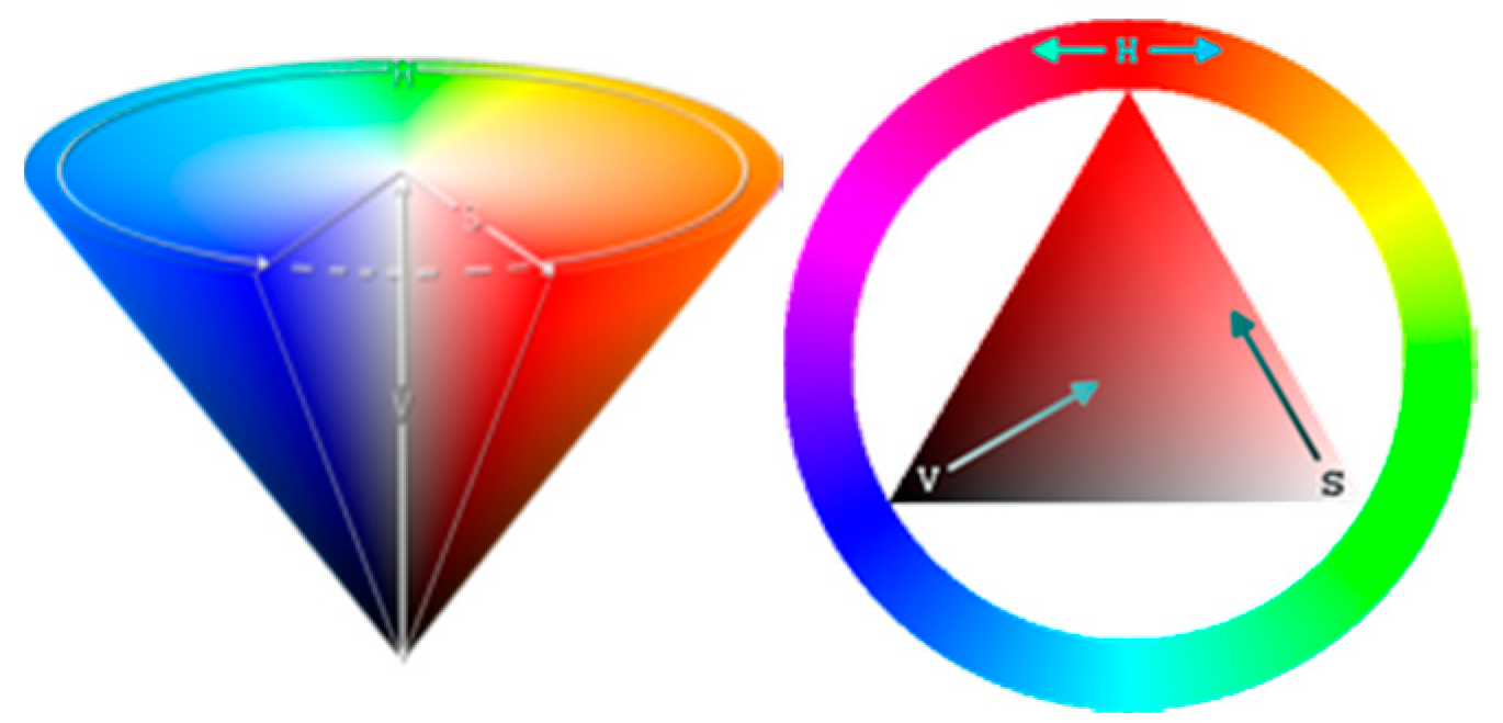
Hue is a basic parameter of color and also the main element in distinguishing material categories in nature. By using different hues to present different categories, this representation will also be more in line with human visual observational habits. Therefore, this method uses the color space description method with hue as an element of color description, such as the HSV (hue, saturation, and value) color space in the color mixing system, the Munsell color system, the practical color co-ordinate system (PCCS), and the natural color system (NCS) within the color appearance system. HSV is also known as HSB (hue, saturation, and brightness). These three-color parameters correspond exactly to the three elements of the subjective color. The HSV color space can be expressed as a cone, as shown in Figure 2. Hue is expressed as an angle around the conical center axis. Saturation is represented as the distance from the center of the cross section of the cone to the point. Brightness is expressed as the distance from the center of the cross section of the cone to the apex. The HSV color space has some advantages, and specific characteristics can be seen in [22]. Therefore, the HSV color space was selected as an example (other cases in the same way), and the following methods in this study were also processed in the HSV color space.

2.3.2. Determining the Hues of Classes

For ground cover classes of interest that are to be simultaneously displayed in an image as different categories, the usual concern for observers is color separability. When the number of classes is small, a short running time is required or the visual accuracy does not have to be too high; the color label can be determined by a more mature coding method of the compiler software, e.g., the color mapping function (colormap) in MATLAB can be used for automatically selecting the category hue.

However, in order to improve visual separability in the output image in the HSV color space, selecting the hue value perspectives around the central axis of the cone would provide a good presentation. For a HSI consisting of $a\times b$ pixels and c bands, the selecting method of hue is as follows:

$$h_j=\frac{360°j}{n}+a$$

(1)

where n denotes the class number, $h_j$ is the hue value of the j-th class color label, and $h_j\in \left[0,360°\right]$; a is the initial phase of hue. The value a can be determined through the supervised information, so it can try to fulfill the required preset colors. Otherwise, the color label assignment method of hyperspectral classification [2,13] can be used in this step.

2.3.3. Determining the Hues of Each Pixel

The bands of the spectral reflection of the ground object of the j-th class are reduced to three bands using manifold learning methods. These three bands are denoted as $V_j^{\prime }$, $S_j^{\prime }$, and $I_j^{\prime }$ according to the significance of the bands, and each of them have the size $a\times b$. To fully utilize the color space and have better visual separability, a separation factor r is introduced into the pixel hue determining method to adjust the differences between similar features.

The separation factor r represents the floating limitation of each pixel’s hue around the hue class. A higher r indicates a greater difference between pixel hues in the same class, along with more chromatism, and a better distance-preserving property of the output image. In addition, a lower r indicates greater differences among the classes of the output image. Theoretically, the range of r can be set as [0, 0.5]. When $r=0$, all the pixel hues are equal to the hues of their relevant classes. When $r=0.5$, the fluctuation range of pixels in each class is exactly half of the hue distance between classes; at this time, the range of all pixels of each class occurs in the entire hue space of the HSV color space. When $r>0.5$, the range of pixels representing different classes in the images will cross. Therefore, we should avoid values within this range except for particular demands. Consequently, to obtain clearer display results, a separation factor r_j of the j-th class is described by the following equation:

$$H_{j,i}=r_j{I}_{j,i}∆h+h_j$$

(2)

$$0<r_j\le 1/3$$

(3)

where $H_{j,i}$ is the hue value of the i-th pixel in the j-th class, $I_{j,i}$ is the result of normalized $I_j$ of the i-th pixel to $\left[-1,1\right]$, and $∆h$ is the category label color difference. Normally, for all categories, $r_j$ is selected as the same value regardless of j.

2.4. The Whole Data Display in the Color Space

The hue value of each pixel is obtained by following the above method. The saturation and brightness of each pixel still need to be determined. After manifold dimension reduction, the data of the first two dimensions in each category are displayed as the saturation and the brightness of each pixel, respectively. In the HSV color space, the value range of saturation $S_j$ and brightness $V_j$ is the normalization of $S_j^{\prime }$ and $V_j^{\prime }$ to $\left[0,1\right]$, as shown in Figure 2. To reduce the overflow problem of color space boundaries, the 2D data needs to be used as the pixel value of saturation and brightness and normalized to $S_j\in \left[0,0.9\right]$ and $V_j\in \left[0.1,1\right]$. Finally, for the pixels of the j-th class, saturation $S_j$ and brightness $V_j$, combined with the hues $H_j$ of each pixel, as described in the previous section, are successively displayed in the three channels of color space. The pixels of the j-th class displayed in the color space $C_j$ with the size of $\left(a,b,3\right)$ are described by the following Equation:

$$C_j=\left[\begin{array}{c}{H}_j\\ S_j\\ V_j\end{array}\right]=\left[\begin{array}{c}{r}_j{I}_j∆h+360°j/n+a\\ S_j\\ V_j\end{array}\right]$$

(4)

3. Experiments and Results

3.1. Hyperspectral Data Sets

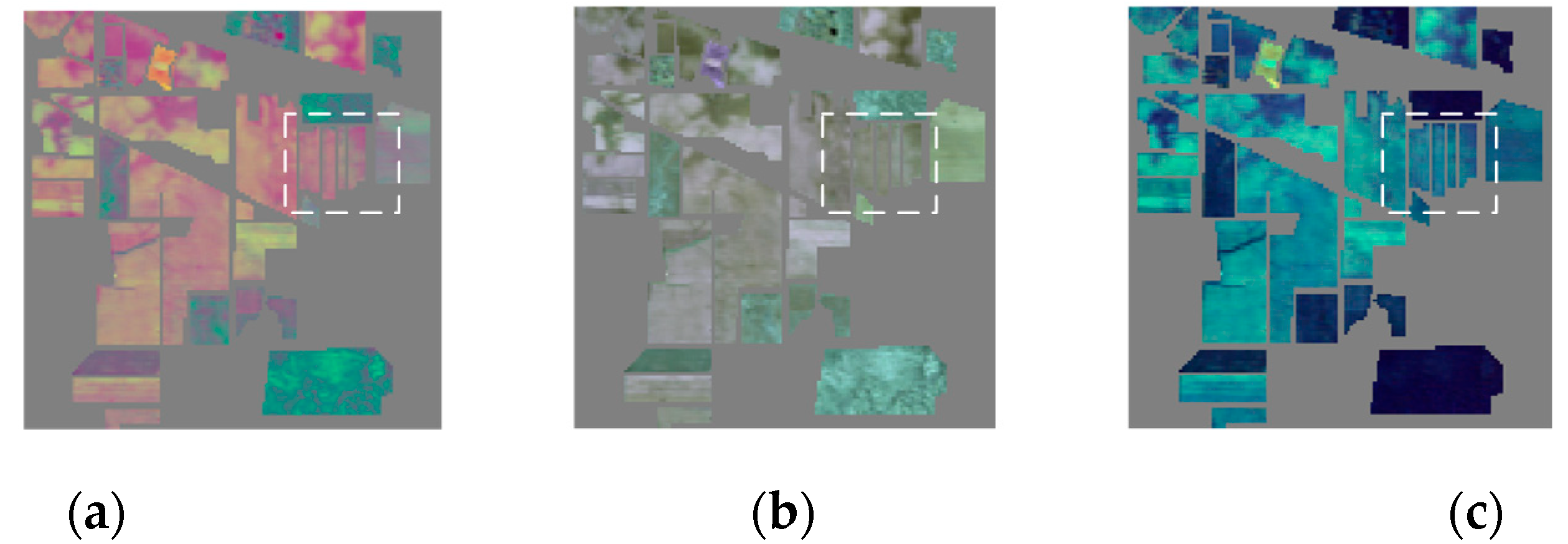
In this study, four supervised hyperspectral remote sensing data were used: Indian Pines, Pavia University, Salinas, and a local area zoomed image from the Salinas image (denoted as SalinasA). The four sets of data were used in experiments after correction and removal of their high noise bands. The single-band grayscale images are shown in Figure 3, and the display results of the hue category label are shown in Figure 4. The experiments were operated on a MATLAB platform using five kinds of manifold algorithms to compare the performance of the different algorithms.

3.2. Evaluation Criteria

Four evaluation criteria were used: the OIF, the distance-preserving property, pixel separability, and the average Euclidean distance between classes. The four criteria are described in some detail below.

• The optimum index factor has often been used in the literature [23] for band selection. The OIF comprehensively considers the information of single-band images and the relevance between various bands. The method of information/redundancy was used in this study to measure the usefulness of the information located in the images. The larger the OIF, the more information the image contains. It is formulated as follows:

  $$OIF={\displaystyle \sum }_{i=1}^{3}std\left(C_i\right)/{\displaystyle \sum }_{i=1,j\ne i}^3{R}_{ij}$$

  (5)

  where $std\left(C_i\right)$ is the standard deviation of Euclidean distance in the color space of the i-th band of image data C, and $R_{ij}$ is the correlation coefficient between the i-th band and the j-th band.
• The distance-preserving property ρ means that the differences in distance between each pixel of the generated images are as correlated as possible between spectral vectors in the HSI data. The image spectral distance-preserving property is good when ρ is closer to 1. The distance-preserving property can be represented as follows [3]:

  $$\rho =\frac{\raisebox{1ex}{$\left(X^{\mathrm{T}}Y\right)$}\!\left/ \!\raisebox{-1ex}{$\left|X\right|$}\right.-\overline{X}\overline{Y}}{std\left(X\right)\times std\left(Y\right)}$$

  (6)

  where vector X is the spectral angle vector of each pair of pixels in the original hyperspectral space. Vector Y is the Euclidean distance between each pair of pixels in the CIELab color space, $\overline{X}$ is the mean of $X$, $\left|X\right|$ is the cardinality of $X$, and std(X) is the standard deviation of X.
• Pixels of the output image should not only show the relationship between pixels but also make the different pixels easily distinguishable. Pixel separability is the evaluation criterion of this property. Pixel separability can be evaluated by the average value δ of the color difference between pixels. The bigger the δ, the more obvious the difference between individual elements and better the between-class separability. The δ can be computed as follows:

  $$\delta ={\left|Y\right|}_1/\left|Y\right|$$

  (7)

  where |Y|₁ and |Y| are the L1 norm and the cardinality of vector Y, respectively.
• λ, the average Euclidean distance between classes, is used to compare the separability between all classes. Larger λ indicates that the categories are more distinguishable. It can be represented as follows:

  $$\lambda =\raisebox{1ex}{$\sum \mathsf{\Delta }d{}^{\prime }$}\!\left/ \!\raisebox{-1ex}{$C_n^2$}\right.$$

  (8)

  where $\mathsf{\Delta }d{}^{\prime }$ is the Euclidean distance between two different classes and $C_n^2=\frac{2}{n!\left(n-2\right)!}$.

3.3. Experimental Results

Four real HSI data sets were used to verify the feasibility of the object-oriented hyperspectral color visualization approach proposed in this paper. Five kinds of manifold algorithms, namely, T-SNE, LE, ISOMAP, LLE, and LTSA, were used for dimension reduction of the proposed method (Section 2.2) to obtain the object-oriented output images. These output images were also compared with traditional data-oriented visualization methods, such as principal component analysis (PCA), fixed linear spectral weighting envelopes (the color matching function (CMF) is the generally used weighting function), and band selection based on optimal basis fitting (referred to as BS).

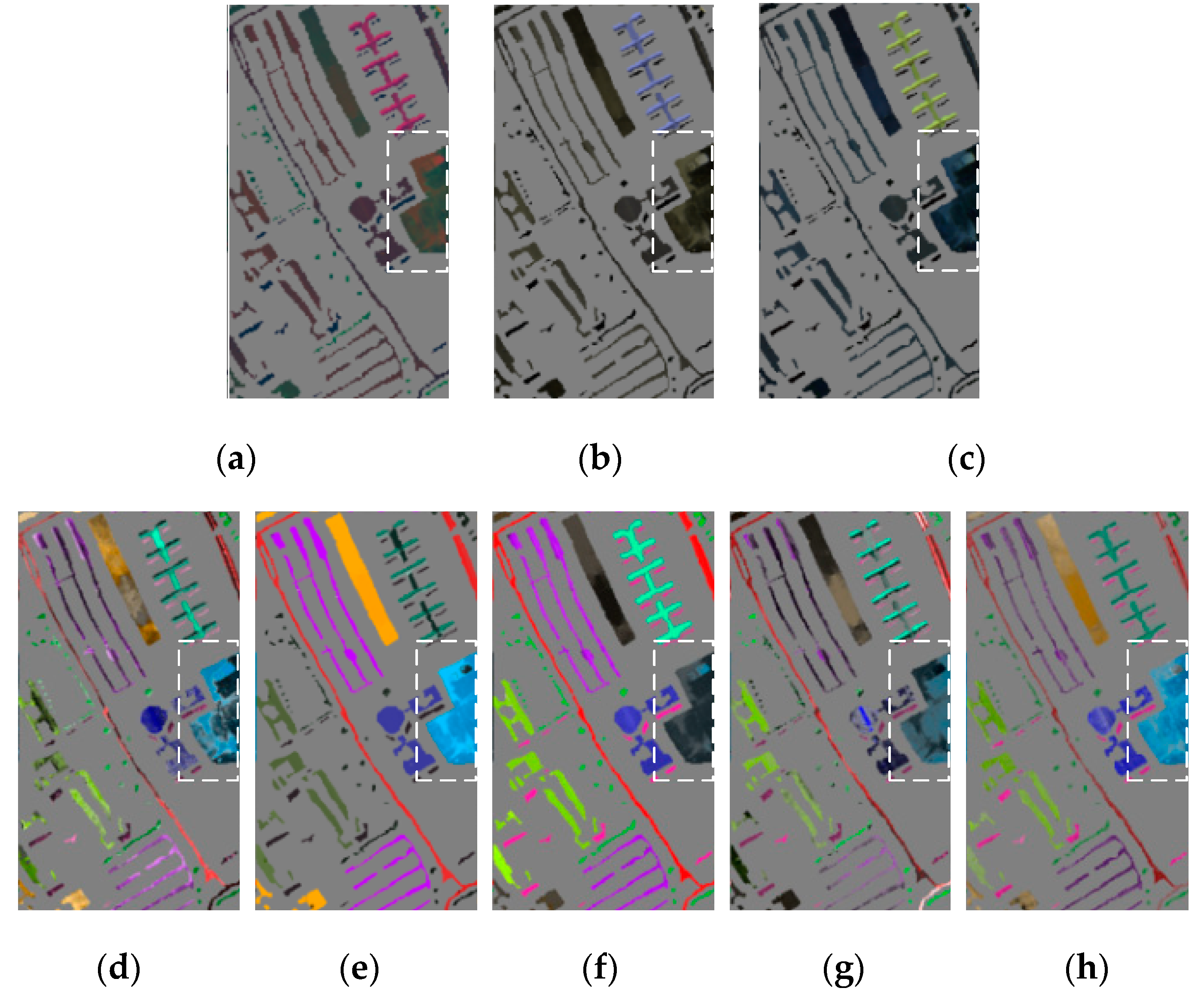
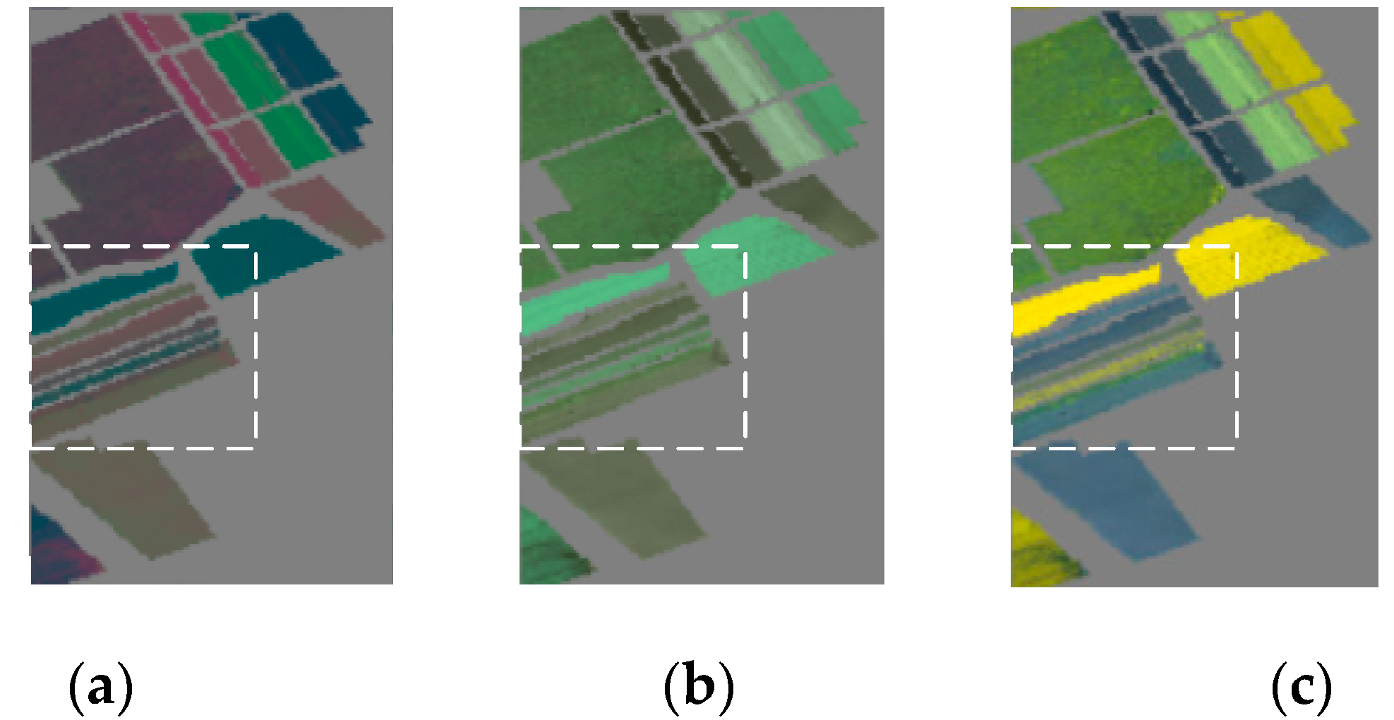
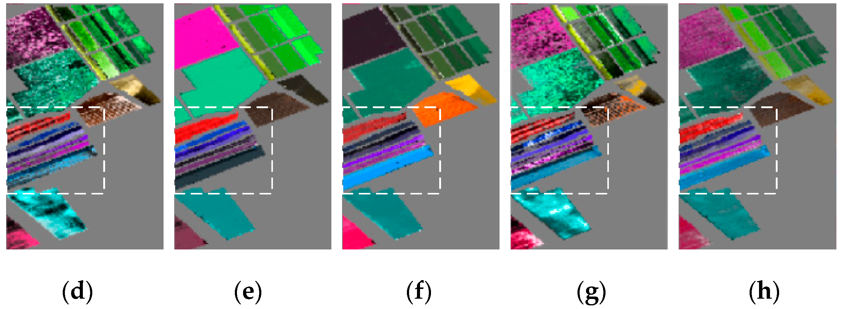
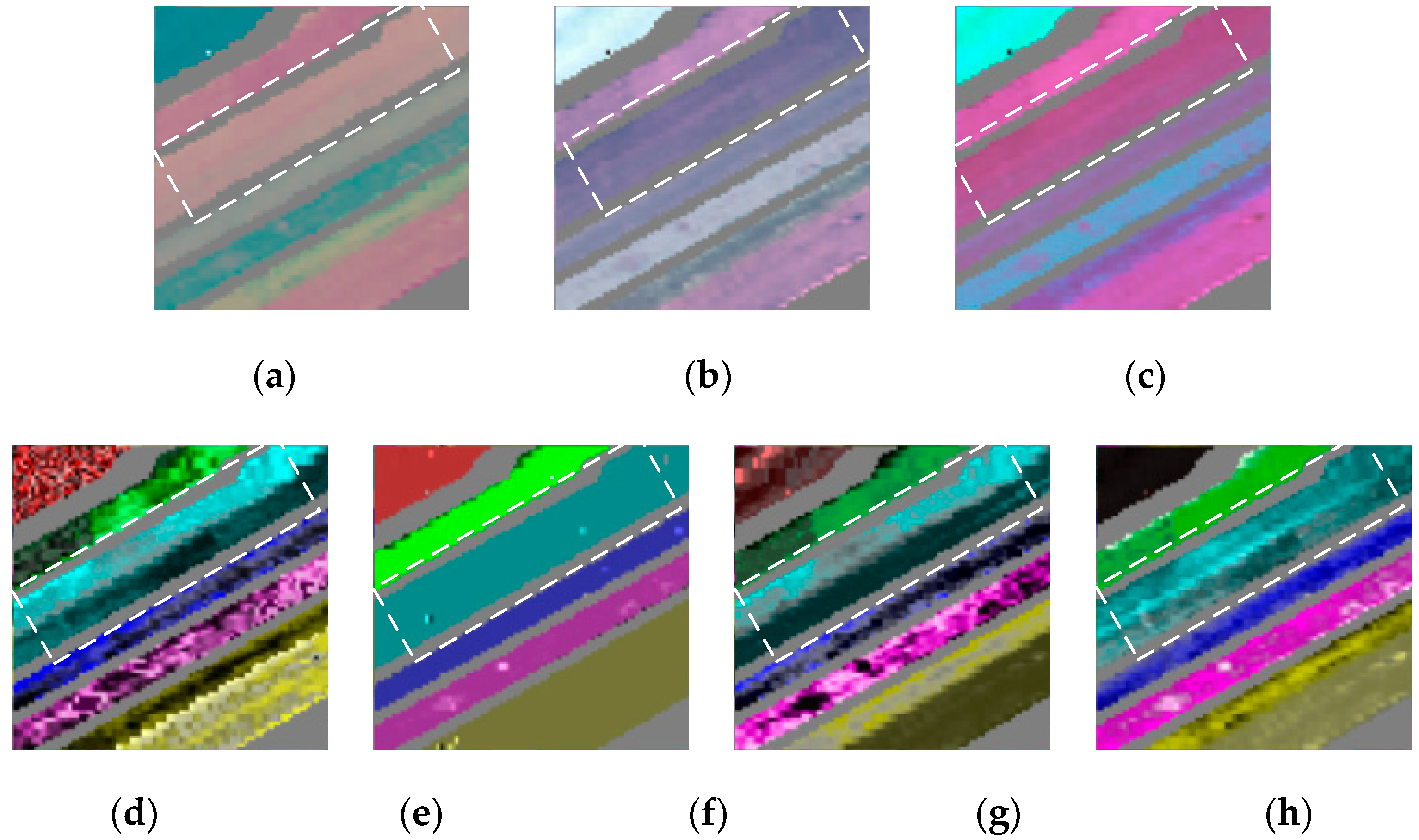
All the experiments were described in HSV color space, without a preset color. The hue class values were selected perspectives around the central axis of the cone. The initial hue phase was $a=0$. The separation factor was $r=0$. The display results for each data set and the color display image for the data-oriented method using PCA, CMF, and BS can be seen in subfigures (a) to (c) in Figure 5, Figure 6, Figure 7 and Figure 8. Furthermore, subfigures (d) to (h) in Figure 5, Figure 6, Figure 7 and Figure 8 display the visualization results of the proposed object-oriented method using the manifold learning method.

As seen in Figure 5, Figure 6, Figure 7 and Figure 8, the proposed object-oriented methods (subfigures (d) to (h) in Figure 5, Figure 6, Figure 7 and Figure 8) were in general visually better in terms of separability of the classes and showed more colorful and vivid ground objects in the images. In this approach, the different classes were, in most cases, displayed clearly (e.g., the ground object classes in the dotted box in Figure 5 and Figure 7), and the pixels of the same class were usually displayed distinctly (e.g., the pixels in the dotted box in Figure 6 and Figure 8). Therefore, the output images for the proposed class-oriented method looked more brightly colored and also had a better eye color perception distance between the classes. Actually, the proposed object-oriented method can generate totally different colors for categories with a similar spectral response. This property directly affects the observers’ ability to distinguish between the different categories. As the display results for each data set make full use of the known information, the object-oriented method has more advantages in visually distinguishing different categories.

The pixel separability of the classes in the output images, which were generated by the proposed object-oriented visualization method, was higher than for most data-oriented approaches. For example, for the three manifold algorithms, i.e., T-SNE, LE, and ISOMAP (subfigures (d), (g), and (h) in Figure 5, Figure 6, Figure 7 and Figure 8), the detailed pixel display effect within the class in the output image was clearer than for the other methods. Thus, these three methods are more suitable for displaying the difference between pixels within the same class. The methods LTSA and LLE (subfigures (e) and (f) in Figure 5, Figure 6, Figure 7 and Figure 8) were weaker than the other methods in terms of displaying the abnormal pixels within the classes. They are more focused on abnormal indications of pixels within classes, and therefore these methods are suitable for occasional special needs.

To describe the visual effect of the various methods more objectively, four evaluation parameters were introduced into the experiment: the amount of information (OIF), correlation coefficient $\rho$, separability $\delta$, and average separability between classes $\lambda$. The calculation results of the output images of the four real HSIs under the four evaluation standards are shown in

Table 1. Optimum Index Factor (OIF).

OIF	Data-Oriented Method			Object-Oriented Method
	PCA	CMF	BS	T-SNE	LE	ISOMAP	LLE	LTSA
Indian	0.1008	0.0091	0.0300	0.4608	0.2641	0.1120	0.1335	0.1476
Pavia	0.0125	0.0133	0.0162	0.3992	0.3405	0.2571	0.1701	0.0903
Salinas	0.0214	0.0099	0.0400	0.5108	0.4568	0.1190	0.1213	0.0957
SalinasA	0.3940	0.0165	0.0281	0.5962	0.2533	0.0904	—	0.1008

,

Table 2. The correlation of the original data ($\mathit{\rho }$).

$\mathit{\rho }$	Data-Oriented Method			Object-Oriented Method
	PCA	CMF	BS	T-SNE	LE	ISOMAP	LLE	LTSA
Indian	0.9306	0.7815	0.9641	0.8326	0.8273	0.7567	0.8956	0.9705
Pavia	0.8482	0.7245	0.8362	0.9707	0.9645	0.9363	0.8823	0.8880
Salinas	0.7167	0.5129	0.9461	0.8544	0.8440	0.7327	0.6638	0.6769
SalinasA	0.6574	0.9158	0.6915	0.8578	0.8455	0.7478	—	0.6272

,

Table 3. Separability between pixels ($\mathit{\delta }$).

$\mathit{\delta }$	Data-Oriented Method			Object-Oriented Method
	PCA	CMF	BS	T-SNE	LE	ISOMAP	LLE	LTSA
Indian	8.76	6.15	14.09	23.83	19.80	14.54	15.78	18.98
Pavia	7.66	6.32	9.65	29.16	29.28	25.10	29.46	33.29
Salinas	4.66	10.16	23.39	19.79	21.07	14.89	19.12	13.36
SalinasA	6.73	19.65	19.65	16.48	14.07	11.73	—	11.58

and

Table 4. Separability between classes ($\lambda$).

$\mathit{\lambda }$	Data-Oriented Method			Object-Oriented Method
	PCA	CMF	BS	T-SNE	LE	ISOMAP	LLE	LTSA
Indian	0.2109	0.1982	0.5483	0.4244	0.4441	0.4152	0.5601	0.7734
Pavia	0.1762	0.3934	0.3848	0.3986	0.3599	0.4958	0.9241	0.7948
Salinas	0.1930	0.3463	0.6002	0.4397	0.4932	0.5262	0.6637	0.6632
SalinasA	0.2402	0.5261	0.6168	0.3972	0.3572	0.6018	—	0.6276

. As can be seen, in comparison with PCA, CMF, and BS, the proposed method, which is based on the application of different manifold algorithms, had higher OIF and λ under most conditions. This means that it obtained the best results in comparison with images generated by the data-oriented approaches. It can be observed that the proposed object-oriented approach could display more information and obtain a better separability between classes. In addition, looking at the results for these two parameters, the location of optimal results was relatively stable, which shows that these two features were not influenced much by the data, at least to some extent. The optimal results for ρ and δ showed the best results with different locations for different data sets, i.e., these two features of the output image depended on the original data to some extent.

The SalinasA data were part of the Salinas data with fewer classes and a smaller image size. It should be noted that the proposed method is designed for large HSIs with multiple classes. Therefore, when the proposed approach is applied on a small image with few classes, like for SalinasA, the advantages of separability between pixels will sometimes not be apparent (see results in Table 2 and Table 3). Furthermore, it can be seen from Figure 5, Figure 6, Figure 7 and Figure 8 that, in comparison with SalinasA, the other HSIs with more classes benefited more in terms of results from the object-oriented method.

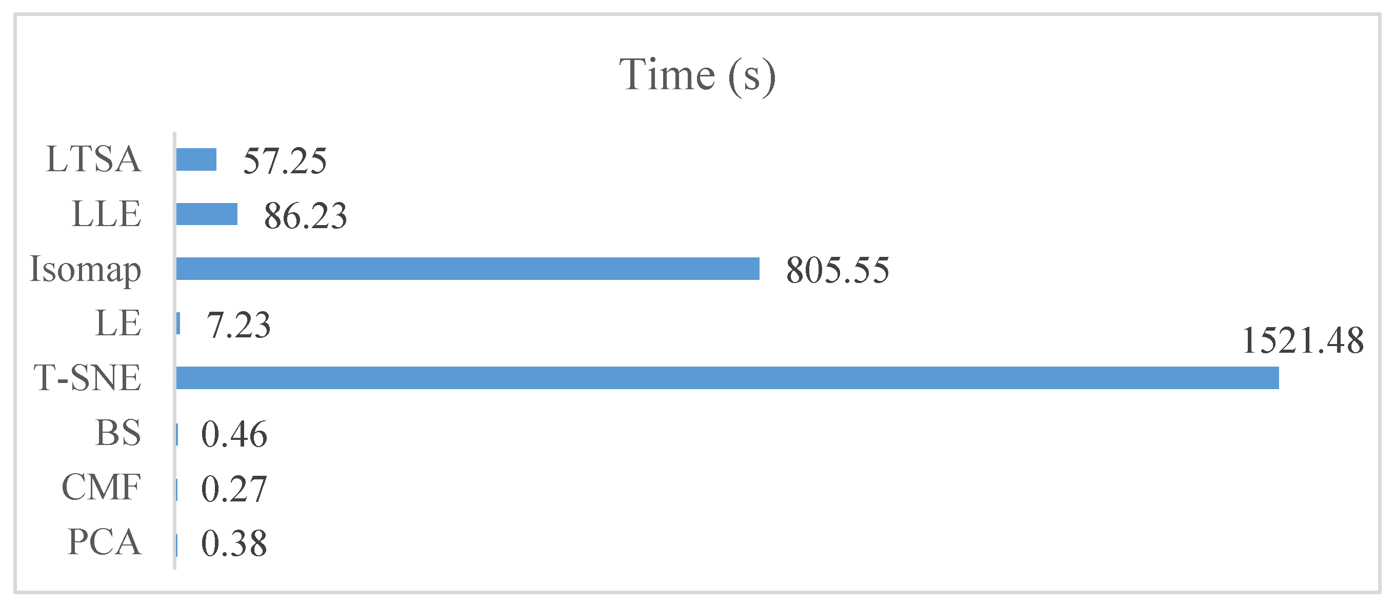
The tables above show that the object-oriented methods performed better than the traditional data-oriented methods. The output images generated by the object-oriented visualization approach contained more information (OIF), had similar relevance to the original data ($\rho$), had better separability between the pixels ($\delta$), and had better separability between the classes ($\lambda$). The manifold algorithms used in these experiments, i.e., T-SNE and LE, showed certain advantages, such as clarity of the information (OIF), good correlation (($\rho$), and better pixel separability ($\delta$). LTSA and LLE demonstrated better separability between classes ($\lambda$). Meanwhile, as shown in Figure 9, T-SNE and ISOMAP consumed longer computing time than the other methods. Therefore, T-SNE and ISOMAP are unsuitable for real-time processing or processing that has requirements regarding the amount of time needed. If no special requirements are needed, the LE algorithm has more advantages.

3.4. The Influence of the Separation Factor on the Images

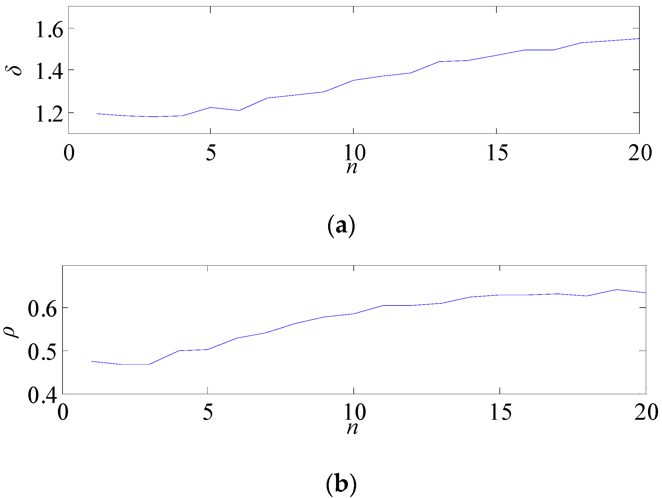
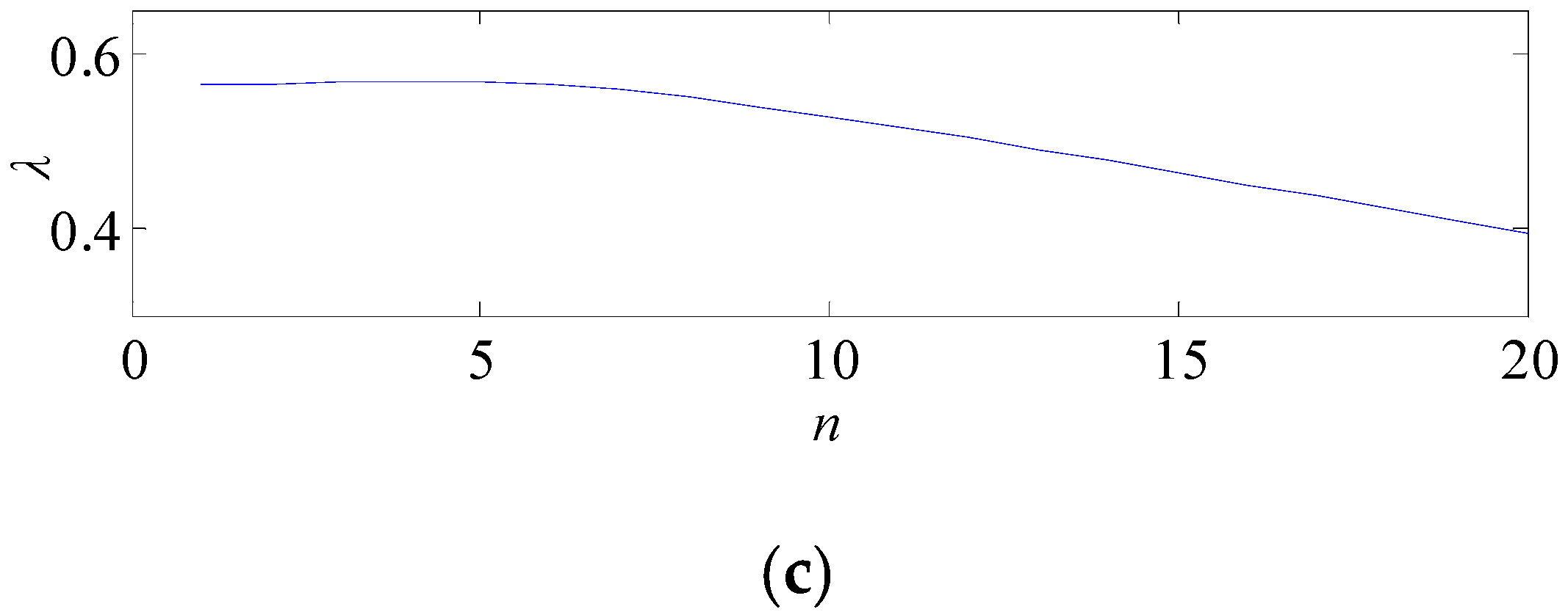
The separation factor r is a constant value in [0, 0.5]. The smaller the value, the better the separability between classes. In contrast, the bigger r, the better the pixel separability within the class and the better the distance-preserving properties that are obtained, meaning that the visual sense of the color of each pixel in the image will be closer to the relational characteristics between each pixel of the original hyperspectral data. When $r_{max}=\mathsf{\Delta }h/4$, $r=n\times r_{max}/20$, $n\subset N$, the relationships between the value of r and the class separability and the correlation within the class are shown in Figure 10.

Figure 11 displays six results for the Indian Pines data with different r values. To avoid the visual confusion of the expression between classes, the biggest r value is $r_{max}=\mathsf{\Delta }h/4$. As shown in Figure 10 and Figure 11, the smaller the r, the easier it will be to distinguish the difference between the classes, and the bigger the r, the better the separability and details of the image. When r is relatively high, this can be problematic, such as shown in Figure 11f. Some color differences in one category are larger than those between different categories. If this value is exceeded, the color expression of pixels will cause confusion and lose significance. Therefore, the value of $r$ should be determined according to the demands of the observers.

4. Discussion

In this paper, an object-oriented visualization method based on manifold methods is proposed for HSI where supervised information is available. Five kinds of manifold algorithms and four HSI data sets were used to verify the feasibility of the proposed approach. The experiments highlighted the effectiveness of the proposed method through subjective and objective evaluations. In subjective evaluations, three manifold algorithms, namely, T-SNE, LE, and ISOMAP, demonstrated sharper detailed pixel display effect within the individual classes in the output images. Thus, these three methods are more suitable for displaying the difference between pixels within the same class. Regarding objective evaluation results, the two manifold algorithms used, i.e., T-SNE and LE, showed clarity of information (OIF), good correlation (ρ) and improved pixel separability (δ) compared to LTSA and LLE.

In contrast to data-oriented processing, where the whole HSI data set with no supervised information is used, the object-oriented visualization method considers the observers’ demands for the HSI displayed with a sense of purpose. Considering the available class information, the proposed method separately processes data from different classes and displays all the classes in the image in an independent fashion. The output images make full use of the supervised information, and an improved visualization is consequently obtained. In addition, the proposed method will play an active role in pest monitoring, disaster early warning, and automatic management of agriculture and forestry.

Furthermore, by adjusting the separation factor, both separability between classes and within classes can be adjusted according to the demands of the observers.

In order to adapt to the nonlinear characteristics of HSI data, manifold algorithms were used in this study. Replacing manifold algorithms with other data processing methods may still work, but the processing method needs to be chosen according to the demand of observers. By comparing experimental results from five commonly used manifold algorithms, it was observed that T-SNE and LE algorithms are superior to other algorithms, but all of them are time-consuming. Therefore, they are unsuitable for real-time processing or processing that has requirements regarding the amount of time needed. Considering the computational load, if no special requirements are needed, the LE algorithm shows the best performance.

References

1. Su, H.; Du, Q.; Du, P. Hyperspectral image visualization using band selection. IEEE Sel. Top. Appl. Earth Obs. Remote Sens. 2014, 7, 2647–2658. [Google Scholar] [CrossRef]
2. Du, Q.; Raksuntorn, N.; Cai, S.; Moorhead, R. Color display for hyperspectral imagery. IEEE Trans. Geosci. Remote Sens. 2008, 46, 1858–1866. [Google Scholar] [CrossRef]
3. Jacobson, N.P.; Gupta, M.R. Design goals and solutions for display of hyperspectral images. IEEE Trans. Geosci. Remote Sens. 2005, 43, 2684–2692. [Google Scholar] [CrossRef]
4. Liao, D.; Qian, Y.; Tang, Y.Y. Constrained manifold learning for hyperspectral imagery visualization. IEEE J. Sel. Top. Appl. Earth Obs. Remote Sens. 2018, 11, 1213–1226. [Google Scholar] [CrossRef] [Green Version]
5. Kang, X.; Duan, P.; Li, S.; Benediktsson, J.A. Decolorization-based hyperspectral image visualization. IEEE Trans. Geosci. Remote Sens. 2018, 56, 4346–4360. [Google Scholar] [CrossRef]
6. Duan, P.; Kang, X.; Li, S. Convolutional neural network for natural color visualization of hyperspectral images. In Proceedings of the IGARSS 2019—2019 IEEE International Geoscience and Remote Sensing Symposium, Yokohama, Japan, 28 July–2 August 2019; pp. 3372–3375. [Google Scholar]
7. Liu, D.; Wang, L.; Benediktsson, J.A. Interactive multi-image colour visualization for hyperspectral imagery. Int. J. Remote Sens. 2017, 38, 1062–1082. [Google Scholar] [CrossRef]
8. Cui, M.; Razddan, A.; Hu, J.; Wonka, P. Interactive hyperspectral image visualization using convex optimization. IEEE Trans. Geosci. Remote Sens. 2009, 47, 1673–1684. [Google Scholar]
9. Mignotte, M. A bicriteria-optimization-approach-based dimensionality-reduction model for the color display of hyperspectral images. IEEE Trans. Geosci. Remote Sens. 2012, 50, 501–513. [Google Scholar] [CrossRef]
10. Duan, P.; Kang, X.; Li, S.; Ghamisi, P. Multichannel pulse-coupled neural network-based hyperspectral image visualization. IEEE Trans. Geosci. Remote Sens. 2019, 58, 1–13. [Google Scholar] [CrossRef]
11. Yang, J.; Zhao, Y.Q.; Chan, J.C.W.; Xiao, L. A multi-scale wavelet 3D-cnn for hyperspectral image super-resolution. Remote Sens. 2019, 11, 1557. [Google Scholar] [CrossRef] [Green Version]
12. Cai, S.; Du, Q.; Moorhead, J.R. Feature-driven multilayer visualization for remotely sensed hyperspectral imagery. IEEE Geosci. Remote Sens. 2010, 48, 3471–3481. [Google Scholar] [CrossRef]
13. Wang, L.; Liu, D.; Zhao, L. A color visualization method based on sparse representation of hyperspectral imagery. Appl. Geophys. 2013, 10, 210–221. [Google Scholar] [CrossRef]
14. Paoletti, M.E.; Haut, J.M.; Plaza, J.; Plaza, A. A new deep convolutional neural network for fast hyperspectral image classification. ISPRS J. Photogramm. Remote Sens. 2018, 145, 120–147. [Google Scholar] [CrossRef]
15. Lunga, D.; Prasad, S.; Crawford, M.M.; Ersoy, O. Manifold-learning-based feature extraction for classification of hyperspectral data: A review of advances in manifold learning. IEEE Signal Process. Mag. 2014, 31, 55–66. [Google Scholar] [CrossRef]
16. Roweis, S.T.; Saul, L.K. Nonlinear dimensionality reduction by locally linear embedding. Sci. Mag. 2000, 290, 2323–2326. [Google Scholar] [CrossRef] [PubMed] [Green Version]
17. Zhang, Z.; Zha, H. Principal manifolds and nonlinear dimension reduction via tangent space alignment. J. Shanghai Univ. 2004, 8, 406–424. [Google Scholar] [CrossRef] [Green Version]
18. Bachmann, C.M.; Ainsworth, T.L.; Fusina, R.A. Improved manifold coordinate representations of large-scale hyperspectral scenes. IEEE Geosci. Remote Sens. 2006, 44, 2786–2803. [Google Scholar] [CrossRef]
19. van der Maaten, L.J.P.; Hinton, G.E. Visualizing high-dimensional data using T-SNE. J. Mach. Learn. Res. 2008, 9, 2579–2605. [Google Scholar]
20. Belkin, D.M.; Niyogi, P. Laplacian eigenmaps for dimensionality reduction and data representation. Neural Comput. 2003, 15, 1373–1396. [Google Scholar] [CrossRef] [Green Version]
21. Healey, C.G. Effective Visualization of Large Multidimensional Datasets. Ph.D. Thesis, The University of British Columbia, Vancouver, BC, Canada, 1996. [Google Scholar]
22. Plataniotis, K.N.; Venetsanopoulos, A.N. Color Image Processing and Applications; Springer: Berlin, Germany, 2000. [Google Scholar]
23. Dwivedi, R.S.; Rao, B.R.M. The selection of the best possible Landsat TM band combination for delineating salt-affected soils. Int. J. Remote Sens. 1992, 13, 2051–2058. [Google Scholar] [CrossRef]
Figure 1. Flow diagram of the object-oriented visualization method of hyperspectral image (HSI).
Applsci 10 03581 g001
Figure 2. The HSV (hue, saturation, and value) color system.
Applsci 10 03581 g002
Figure 3. The 80th band of the HSIs. (a) Indian Pines; (b) Pavia University; (c) Salinas; (d) SalinasA.
Applsci 10 03581 g003
Figure 4. Color labels for the classes. (a) Indian Pines; (b) Pavia University; (c) Salinas; (d) SalinasA.
Applsci 10 03581 g004
Figure 5. Visualization result for Indian Pines. (a) Principal component analysis (PCA); (b) color matching function (CMF); (c) band selection; (d) t-distributed stochastic neighbor embedding (T-SNE); (e) local tangent space alignment (LTSA); (f) locally linear embedding (LLE); (g) Laplacian eigenmaps (LE); (h) isometric feature mapping (ISOMAP).
Applsci 10 03581 g005aApplsci 10 03581 g005b
Figure 6. Visualization result for Pavia University. (a) PCA; (b) CMF; (c) band selection; (d) T-SNE; (e) LTSA; (f) LLE; (g) LE; (h) ISOMAP.
Applsci 10 03581 g006
Figure 7. Visualization result for Salinas. (a) PCA; (b) CMF; (c) band selection; (d) T-SNE; (e) LTSA; (f) LLE; (g) LE; (h) ISOMAP.
Applsci 10 03581 g007aApplsci 10 03581 g007b
Figure 8. Visualization results for SalinasA. (a) PCA; (b) CMF; (c) band selection; (d) T-SNE; (e) LTSA; (f) LE; (g) ISOMAP.
Applsci 10 03581 g008
Figure 9. Average running time for each manifold algorithm.
Applsci 10 03581 g009
Figure 10. The relationship between r and (a) δ , (b) ρ , or (c) λ .
Applsci 10 03581 g010aApplsci 10 03581 g010b
Figure 11. Indian Pines image display results under six different r values. (a) r = 0; (b) r = 0.0038; (c) r = 0.0077; (d) r = 0.0115; (e) r = 0.0154; (f) r = 0.0183.
Applsci 10 03581 g011