Estimation of Wind Turbine Angular Velocity Remotely Found on Video Mining and Convolutional Neural Network

 , , and
Abstract
:1. Introduction
2. Related Works
3. Proposed Model
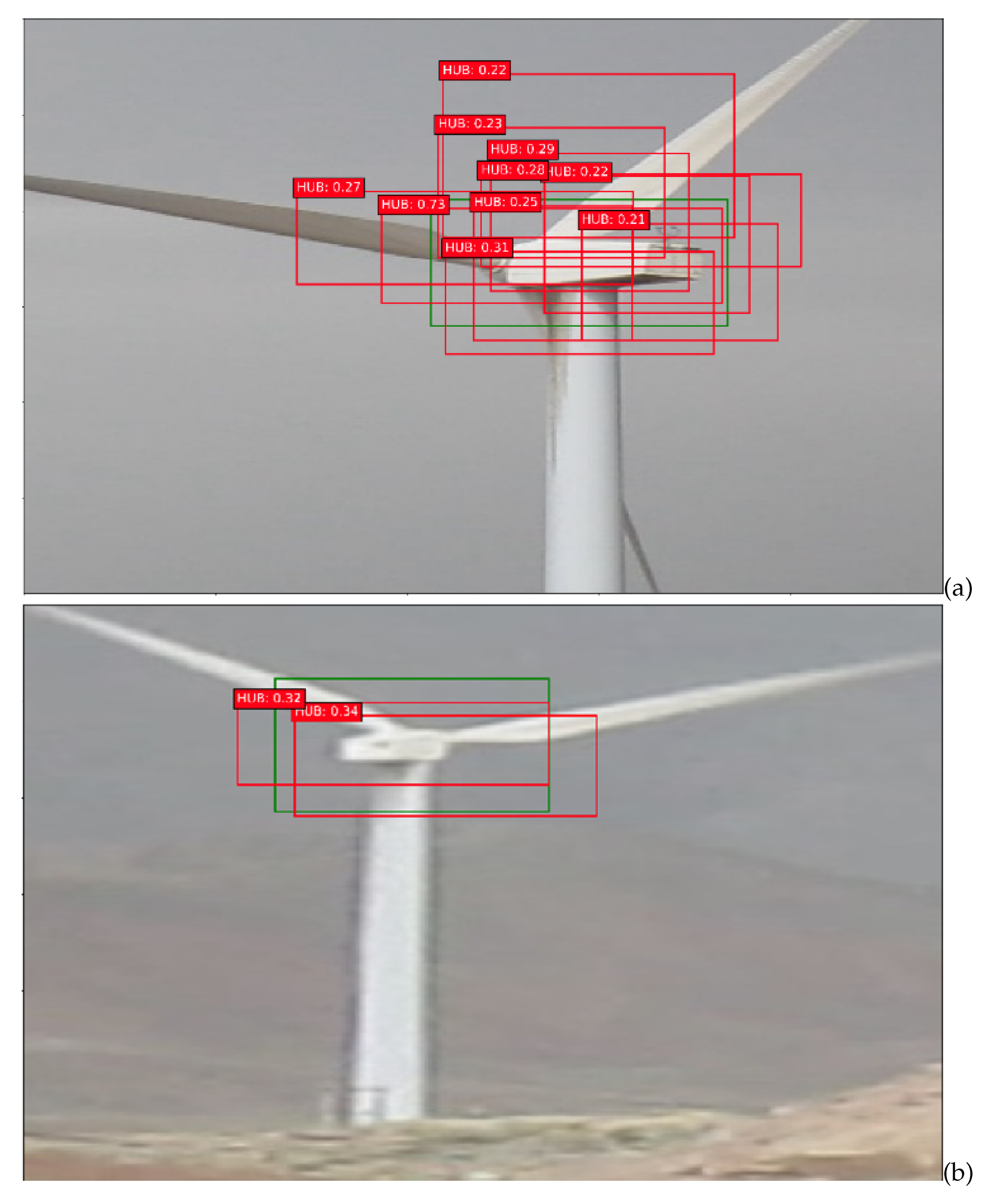
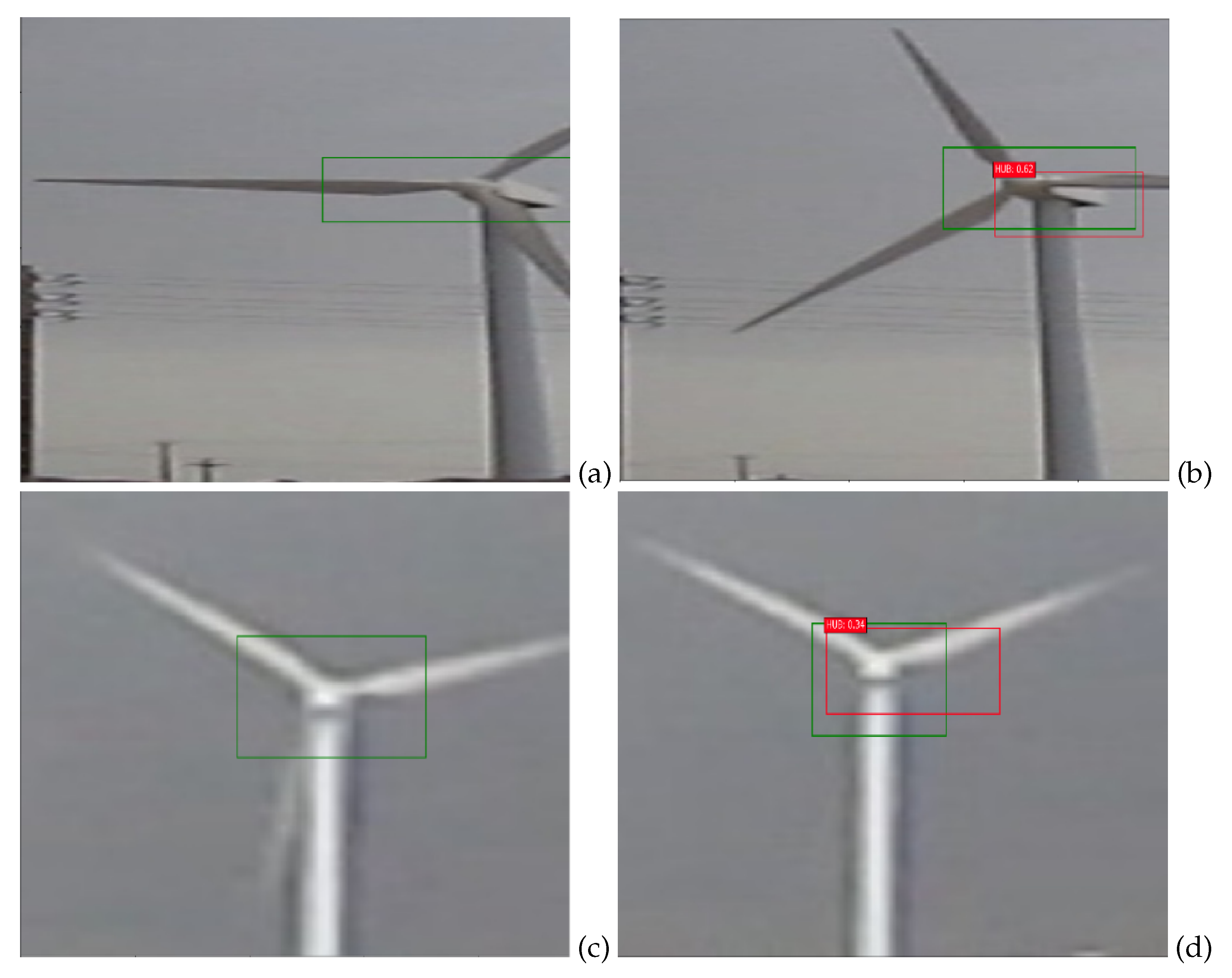
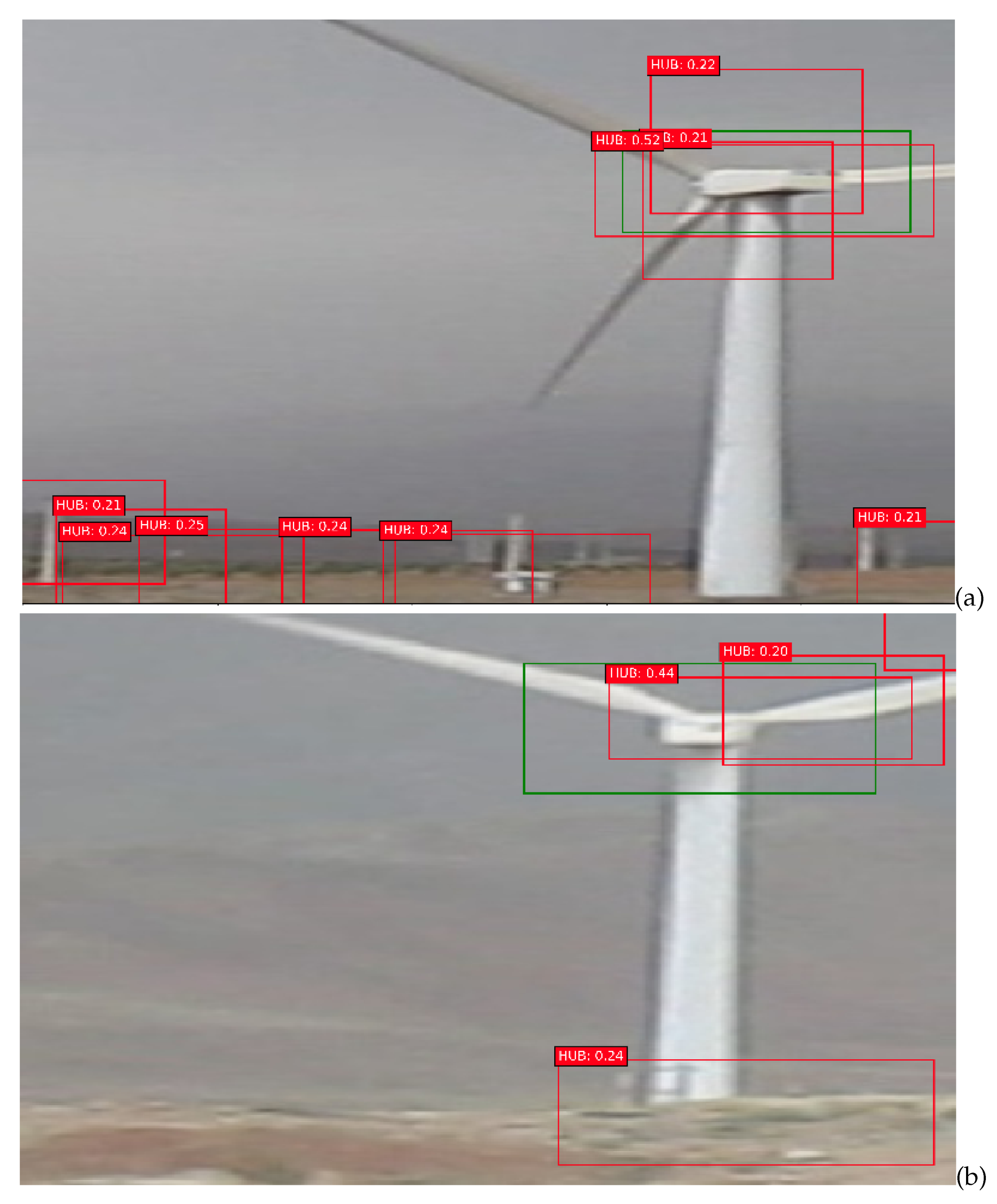
3.1. Hub Object Detection
Selecting the Best Object
3.2. Blade and Non-Blade Binary Classification
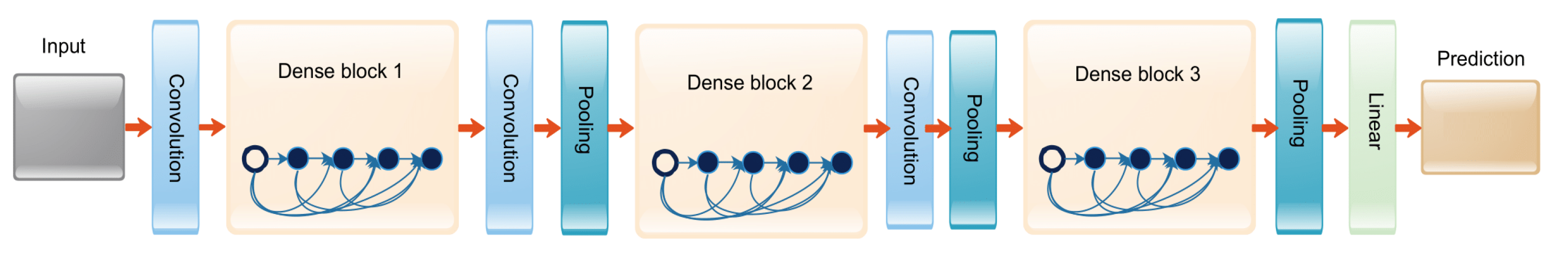
3.2.1. ResNet
3.2.2. DenseNet
3.2.3. InceptionV3
3.2.4. SqueezeNet
3.3. Blade Angular Velocity Estimation Method
4. Experimental Results
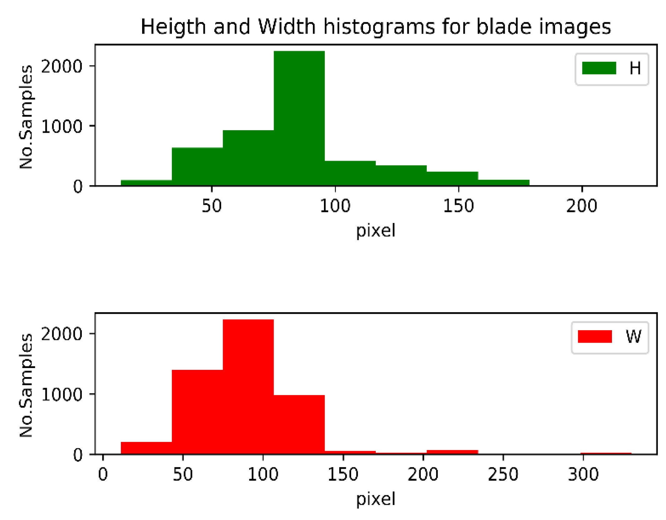
4.1. Dataset
4.2. Hub Object Detection
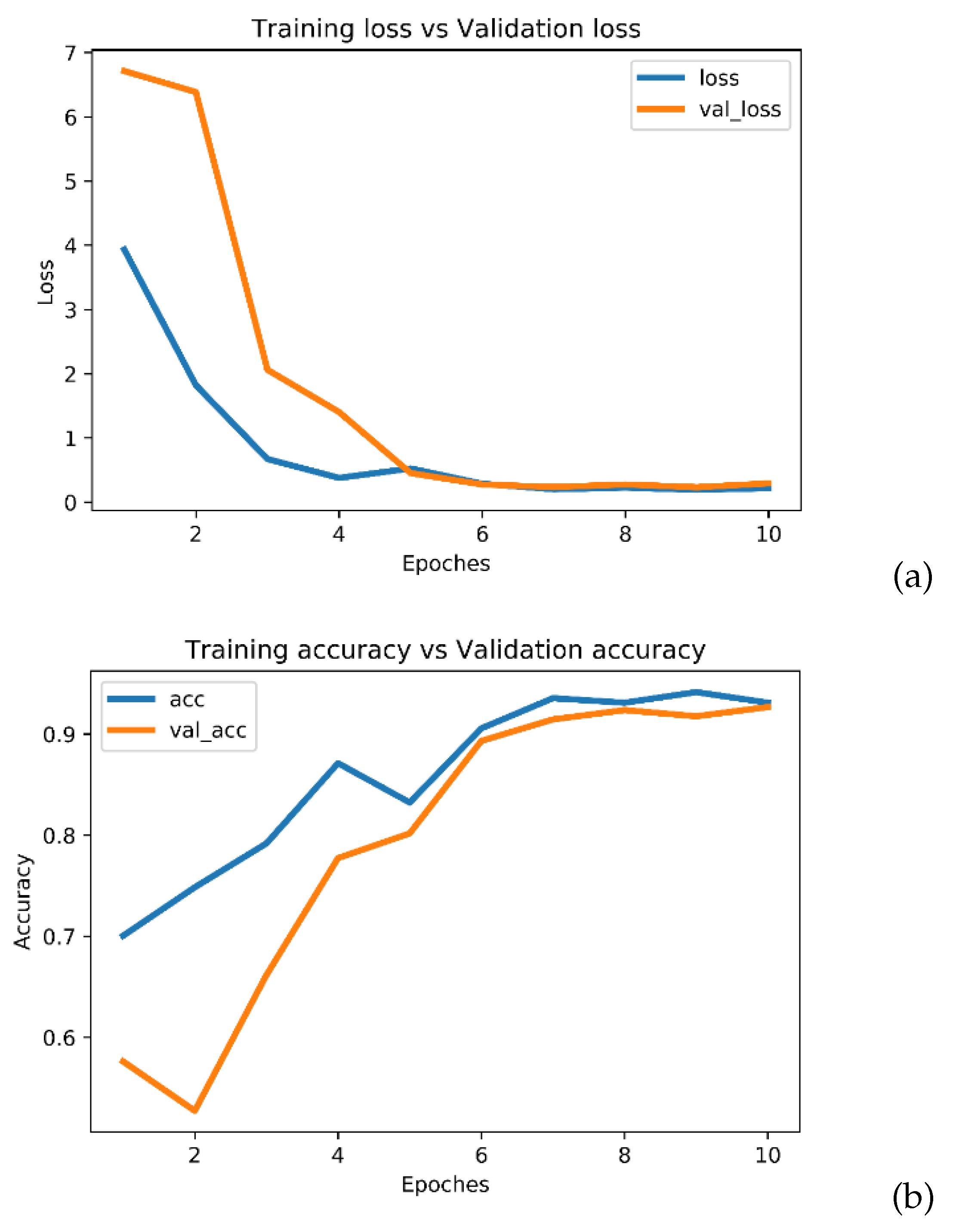
4.3. Blade/Non-Blade Classification
4.4. Angular Velocity Estimation
5. Conclusions and Future Work
Author Contributions
Funding
Conflicts of Interest
References
- Moccia, J.; Arapogianni, A.; Wilkes, J.; Kjaer, C.; Gruet, R.; Azau, S.; Scola, J. Pure power. wind energy targets for 2020 and 2030. INIS 2011, 43. [Google Scholar]
- Lauha, F.; Steve, S.; Sgruti, S.; Limig, Q. Global Wind Report Annual Market Update 2013; Global Wind Energy Council: Brussels, Belgium, 2012. [Google Scholar]
- Li, D.; Ho, S.C.M.; Song, G.; Ren, L.; Li, H. A review of damage detection methods for wind turbine blades. Smart Mater. Struct. 2015, 24, 033001. [Google Scholar] [CrossRef]
- Qiao, W.; Lu, D. A survey on wind turbine condition monitoring and fault diagnosis—Part I: Components and subsystems. IEEE Trans. Ind. Electron. 2015, 62, 6536–6545. [Google Scholar] [CrossRef]
- Drewry, M.A.; Georgiou, G. A review of NDT techniques for wind turbines. Insight-Non-Destr. Test. Cond. Monit. 2007, 49, 137–141. [Google Scholar] [CrossRef] [Green Version]
- Bahaghighat, M.; Motamedi, S.A. Vision inspection and monitoring of wind turbine farms in emerging smart grids. Facta Univ. Ser. Electron. Energ. 2018, 31, 287–301. [Google Scholar] [CrossRef] [Green Version]
- Abedini, F.; Bahaghighat, M.; S’hoyan, M. Wind turbine tower detection using feature descriptors and deep learning. Facta Univ. Ser. Electron. Energ. 2019, 33, 133–153. [Google Scholar] [CrossRef]
- Bahaghighat, M.; Motamedi, S.A.; Xin, Q. Image Transmission over Cognitive Radio Networks for Smart Grid Applications. Appl. Sci. 2019, 9, 5498. [Google Scholar] [CrossRef] [Green Version]
- Esmaeili Kelishomi, A.; Garmabaki, A.; Bahaghighat, M.; Dong, J. Mobile user indoor-outdoor detection through physical daily activities. Sensors 2019, 19, 511. [Google Scholar] [CrossRef] [Green Version]
- Bahaghighat, M.; Motamedi, S.A. PSNR enhancement in image streaming over cognitive radio sensor networks. Etri J. 2017, 39, 683–694. [Google Scholar] [CrossRef] [Green Version]
- Bahaghighat, M.; Motamedi, S.A. IT-MAC: Enhanced MAC Layer for Image Transmission Over Cognitive Radio Sensor Networks. Int. J. Comput. Sci. Inf. Secur. 2016, 14, 234. [Google Scholar]
- Naghdehforushha, S.A.; Bahaghighat, M.; Salehifar, M.R.; Kazemi, H. Design of planar plate monopole antenna with vertical rectangular cross-sectional plates for ultra-wideband communications. Facta Univ.-Ser. Electron. Energ. 2018, 31, 641–650. [Google Scholar] [CrossRef] [Green Version]
- Bahaghighat, M.; Naghdehforushha, A.; Salehifar, M.R.; Mirfattahi, M. Designing straight coaxial connectors for feeder and jumpers in cellular mobile base stations. Acta Tech. Napoc. Electron.-Telecomun. 2018, 59, 1–5. [Google Scholar]
- Hasani, S.; Bahaghighat, M.; Mirfatahia, M. The mediating effect of the brand on the relationship between social network marketing and consumer behavior. Acta Tech. Napoc. 2019, 60, 1–6. [Google Scholar]
- Igba, J.; Alemzadeh, K.; Durugbo, C.; Eiriksson, E.T. Analysing RMS and peak values of vibration signals for condition monitoring of wind turbine gearboxes. Renew. Energy 2016, 91, 90–106. [Google Scholar] [CrossRef] [Green Version]
- Li, S.; Wunsch, D.C.; O’Hair, E.A.; Giesselmann, M.G. Using neural networks to estimate wind turbine power generation. IEEE Trans. Energy Convers. 2001, 16, 276–282. [Google Scholar]
- Watson, S.; Xiang, J. Real-time condition monitoring of offshore wind turbines. In Proceedings of the European Wind Energy Conference & Exhibition, Athens, Greece, 2 March 2006; pp. 647–654. [Google Scholar]
- Rumsey, M.A.; Paquette, J.A. Structural health monitoring of wind turbine blades. In Smart Sensor Phenomena, Technology, Networks, and Systems 2008; International Society for Optics and Photonics: San Diego, CA, USA, 2008; Volume 6933, p. 69330E. [Google Scholar]
- Qiao, W.; Lu, D. A survey on wind turbine condition monitoring and fault diagnosis—Part II: Signals and signal processing methods. IEEE Trans. Ind. Electron. 2015, 62, 6546–6557. [Google Scholar] [CrossRef]
- Verbruggen, T. Wind Turbine Operation & Maintenance Based on Condition Monitoring WT-Ω; Final Report, April; ECN, Energy Research Center of the Netherlands: Sint Maartensvlotbrug, The Netherlands, 2003. [Google Scholar]
- Ribrant, J.; Bertling, L. Survey of failures in wind power systems with focus on Swedish wind power plants during 1997–2005. In Proceedings of the Power Engineering Society General Meeting, Tampa, FL, USA, 24–28 June 2007; pp. 1–8. [Google Scholar]
- Grubic, S.; Aller, J.M.; Lu, B.; Habetler, T.G. A survey on testing and monitoring methods for stator insulation systems of low-voltage induction machines focusing on turn insulation problems. IEEE Trans. Ind. Electron. 2008, 55, 4127–4136. [Google Scholar] [CrossRef] [Green Version]
- Grubic, S.; Aller, J.; Lu, B.; Habetler, T. A survey of testing and monitoring methods for stator insulation systems in induction machines. In Proceedings of the Conference on Condition Monitoring and Diagnosis, Beijing, China, 21 April 2008; pp. 196–203. [Google Scholar]
- Lading, L.; McGugan, M.; Sendrup, P.; Rheinländer, J.; Rusborg, J. Fundamentals for Remote Structural Health Monitoring of Wind Turbine Blades—A Preproject, Annex B: Sensors and Non-Destructive Testing Methods for Damage Detection in Wind Turbine Blades; Risø National Laboratory: Roskilde, Denmark, 2002. [Google Scholar]
- Kristensen, O.J.; McGugan, M.; Sendrup, P.; Rheinländer, J.; Rusborg, J.; Hansen, A.M.; Debel, C.P.; Sørensen, B.F. Fundamentals for Remote Structural Health Monitoring of Wind Turbine Blades—A Preproject Annex E—Full-Scale Test of Wind Turbine Blade, Using Sensors and NDT; Risø National Laboratory: Roskilde, Denmark, 2002. [Google Scholar]
- McGugan, M.; Larsen, G.C.; Sørensen, B.F.; Borum, K.K.; Engelhardt, J. Fundamentals for Remote Condition Monitoring of Offshore Wind Turbines; Danmarks Tekniske Universitet: Riso National laboratorie, Denmark, 2008. [Google Scholar]
- Gandhi, A.; Corrigan, T.; Parsa, L. Recent advances in modeling and online detection of stator interturn faults in electrical motors. IEEE Trans. Ind. Electron. 2011, 58, 1564–1575. [Google Scholar] [CrossRef]
- Wang, L.; Zhang, Z. Automatic detection of wind turbine blade surface cracks based on uav-taken images. IEEE Trans. Ind. Electron. 2017, 64, 7293–7303. [Google Scholar] [CrossRef]
- Stokkeland, M. A Computer Vision Approach for Autonomous Wind Turbine Inspection Using a Multicopter. Master’s Thesis, Institutt for Teknisk Kybernetikk, Trondheim, Norway, 2014. [Google Scholar]
- Takeki, A.; Trinh, T.T.; Yoshihashi, R.; Kawakami, R.; Iida, M.; Naemura, T. Combining deep features for object detection at various scales: Finding small birds in landscape images. IPSJ Trans. Comput. Vis. Appl. 2016, 8, 5. [Google Scholar] [CrossRef] [Green Version]
- Wei, L.; Mirzaei, G.; Majid, M.W.; Jamali, M.M.; Ross, J.; Gorsevski, P.V.; Bingman, V.P. Birds/bats movement tracking with IR camera for wind farm applications. In Proceedings of the 2014 IEEE International Symposium on Circuits and Systems (ISCAS), Melbourne, Australia, 27 March 2014; pp. 341–344. [Google Scholar]
- Zhang, Z.; Verma, A.; Kusiak, A. Fault analysis and condition monitoring of the wind turbine gearbox. IEEE Trans. Energy Convers. 2012, 27, 526–535. [Google Scholar] [CrossRef]
- Castellani, F.; Garibaldi, L.; Daga, A.P.; Astolfi, D.; Natili, F. Diagnosis of Faulty Wind Turbine Bearings Using Tower Vibration Measurements. Energies 2020, 13, 1474. [Google Scholar] [CrossRef] [Green Version]
- Seo, K.H.; Park, Y.; Yun, S.; Park, S.; Park, J.W. Vibration occurrence estimation and avoidance for vision inspection system. In Robot Intelligence Technology and Applications 2; Springer: New York, NY, USA, 2014; pp. 633–641. [Google Scholar]
- Yang, H.; Gu, Q.; Aoyama, T.; Takaki, T.; Ishii, I. Dynamics-based stereo visual inspection using multidimensional modal analysis. IEEE Sens. J. 2013, 13, 4831–4843. [Google Scholar] [CrossRef]
- Bahaghighat, M.; Abedini, F.; S’hoyan, M.; Molnar, A.J. Vision Inspection of Bottle Caps in Drink Factories Using Convolutional Neural Networks. In Proceedings of the 2019 IEEE 15th International Conference on Intelligent Computer Communication and Processing (ICCP), Cluj-Napoca, Romania, 5–7 September 2019; pp. 381–385. [Google Scholar]
- Bahaghighat, M.; Mirfattahi, M.; Akbari, L.; Babaie, M. Designing quality control system based on vision inspection in pharmaceutical product lines. In Proceedings of the 2018 International Conference on Computing, Mathematics and Engineering Technologies (iCoMET), Sukkur, Pakistan, 3–4 March 2018; pp. 1–4. [Google Scholar]
- Akbari, R.; Bahaghighat, M.K.; Mohammadi, J. Legendre moments for face identification based on single image per person. In Proceedings of the 2010 2nd International Conference on Signal Processing Systems (ICSPS 2010), Dalian, China, 5–7 July 2010; Volume 1. [Google Scholar]
- Mohammadi, J.; Akbari, R. Vehicle speed estimation based on the image motion blur using radon transform. In Proceedings of the 2010 2nd International Conference on Signal Processing Systems (ICSPS 2010), Dalian, China, 5–7 July 2010; Volume 1. [Google Scholar]
- Bahaghighat, M.K.; Mohammadi, J. Novel approach for baseline detection and Text line segmentation. Int. J. Comput. Appl. 2012, 51, 9–16. [Google Scholar]
- Karami, E.; Prasad, S.; Shehata, M. Image matching using SIFT, SURF, BRIEF and ORB: Performance comparison for distorted images. arXiv 2017, arXiv:1710.02726. [Google Scholar]
- Erhan, D.; Szegedy, C.; Toshev, A.; Anguelov, D. Scalable object detection using deep neural networks. In Proceedings of the IEEE Conference on Computer Vision and Pattern Recognition, NW, Washington, DC, USA, 24–27 June 2014; pp. 2147–2154. [Google Scholar]
- Bahaghighat, M.K.; Sahba, F.; Tehrani, E. Textdependent Speaker Recognition by Combination of LBG VQ and DTW for Persian language. Int. J. Comput. Appl. 2012, 51, 23. [Google Scholar]
- Ghorbani, M.; Bahaghighat, M.; Xin, Q.; Özen, F. ConvLSTMConv network: A deep learning approach for sentiment analysis in cloud computing. J. Cloud Comput. 2020, 9, 1–12. [Google Scholar] [CrossRef] [Green Version]
- Bahaghighat, M.; Akbari, L.; Xin, Q. A machine learning-based approach for counting blister cards within drug packages. IEEE Access 2019, 7, 83785–83796. [Google Scholar] [CrossRef]
- Sajadi, M.S.S.; Babaie, M.; Bahaghighat, M. Design and implementation of fuzzy supervisor controller on optimized DC machine driver. In Proceedings of the 2018 8th Conference of AI & Robotics and 10th RoboCup Iranopen International Symposium (IRANOPEN), Qazvin, Iran, 10 April 2018; pp. 26–31. [Google Scholar]
- Liu, W.; Anguelov, D.; Erhan, D.; Szegedy, C.; Reed, S.; Fu, C.Y.; Berg, A.C. Ssd: Single shot multibox detector. In Proceedings of the European Conference on Computer Vision, Amsterdam, The Netherlands, 8–16 October 2016; pp. 21–37. [Google Scholar]
- Simonyan, K.; Zisserman, A. Very deep convolutional networks for large-scale image recognition. arXiv 2014, arXiv:1409.1556. [Google Scholar]
- Jeong, J.; Park, H.; Kwak, N. Enhancement of SSD by concatenating feature maps for object detection. arXiv 2017, arXiv:1705.09587. [Google Scholar]
- Babaie, M.; Shiri, M.E.; Bahaghighat, M. A new descriptor for UAV images mapping by applying discrete local radon. In Proceedings of the 2018 8th Conference of AI & Robotics and 10th RoboCup Iranopen International Symposium (IRANOPEN), Qazvin, Iran, 10 April 2018; pp. 52–56. [Google Scholar]
- Karimimehr, N.; Shirazi, A.A.B. Fingerprint image enhancement using gabor wavelet transform. In Proceedings of the 2010 18th Iranian Conference on Electrical Engineering (ICEE), Isfahan, Iran, 11–13 May 2010; pp. 316–320. [Google Scholar]
- Bahaghighat, M.K.; Akbari, R. Fingerprint image enhancement using GWT and DMF. In Proceedings of the 2010 2nd International Conference on Signal Processing Systems (ICSPS), Dalian, China, 5–7 July 2010; Volume 1. [Google Scholar]
- Huang, D.Y.; Hu, W.C.; Chang, S.H. Gabor filter-based hand-pose angle estimation for hand gesture recognition under varying illumination. Exp. Syst. Appl. 2011, 38, 6031–6042. [Google Scholar] [CrossRef]
- Affonso, C.; Rossi, A.L.D.; Vieira, F.H.A.; de Leon Ferreira, A.C.P. Deep learning for biological image classification. Exp. Syst. Appl. 2017, 85, 114–122. [Google Scholar] [CrossRef]
- Gysel, P.; Motamedi, M.; Ghiasi, S. Hardware-oriented approximation of convolutional neural networks. arXiv 2016, arXiv:1604.03168. [Google Scholar]
- Szegedy, C.; Ioffe, S.; Vanhoucke, V.; Alemi, A.A. Inception-v4, Inception-Resnet and the Impact of Residual Connections on Learning. In Proceedings of the Thirty-First AAAI Conference on Artificial Intelligence (AAAI-17), San Francisco, CA, USA, 4–9 February 2017; Volume 4, p. 12. [Google Scholar]
- Huang, G.; Liu, Z.; Van Der Maaten, L.; Weinberger, K.Q. Densely Connected Convolutional Networks. In Proceedings of the CVPR, Honolulu, HI, USA, 21–26 July 2017; Volume 1, p. 3. [Google Scholar]
- Jégou, S.; Drozdzal, M.; Vazquez, D.; Romero, A.; Bengio, Y. The one hundred layers tiramisu: Fully convolutional densenets for semantic segmentation. In Proceedings of the 2017 IEEE Conference on Computer Vision and Pattern Recognition Workshops (CVPRW), Honolulu, HI, USA, 21–26 July 2017; pp. 1175–1183. [Google Scholar]
- Krizhevsky, A.; Hinton, G. Learning Multiple Layers of Features From Tiny Images; Technical Report; Citeseer: State College, PA, USA, 2009. [Google Scholar]
- Szegedy, C.; Vanhoucke, V.; Ioffe, S.; Shlens, J.; Wojna, Z. Rethinking the inception architecture for computer vision. In Proceedings of the IEEE Conference on Computer Vision and Pattern Recognition, Las Vegas, NV, USA, 26 June–1 July 2016; pp. 2818–2826. [Google Scholar]
- Iandola, F.N.; Han, S.; Moskewicz, M.W.; Ashraf, K.; Dally, W.J.; Keutzer, K. Squeezenet: Alexnet-level accuracy with 50x fewer parameters and <0.5 mb model size. arXiv 2016, arXiv:1602.07360. [Google Scholar]
- Wu, W.; Wu, A.; Zheng, W.S. Light Person Re-Identification by Multi-Cue Tiny Net. In Proceedings of the 2018 25th IEEE International Conference on Image Processing (ICIP), Athens, Greece, 7–10 October 2018; pp. 1643–1647. [Google Scholar]
- Agoes, A.S.; Hu, Z.; Matsunaga, N. Fine tuning based squeezenet for vehicle classification. In Proceedings of the International Conference on Advances in Image Processing, Bangkok, Thailand, 25–27 August 2017; pp. 14–18. [Google Scholar]
- Tzutalin. Git Code: LabelImg. 2015. Available online: https://github.com/tzutalin/labelImg/blob/master/README.rst (accessed on 15 April 2020).
- Soudani, A.; Barhoumi, W. An Image-based Segmentation Recommender using Crowdsourcing and Transfer Learning for Skin Lesion Extraction. Exp. Syst. Appl. 2018, 105, 233–261. [Google Scholar] [CrossRef]
- Nweke, H.F.; Teh, Y.W.; Al-Garadi, M.A.; Alo, U.R. Deep Learning Algorithms for Human Activity Recognition using Mobile and Wearable Sensor Networks: State of the Art and Research Challenges. Exp. Syst. Appl. 2018, 105, 233–261. [Google Scholar] [CrossRef]
- Felzenszwalb, P.F.; Girshick, R.B.; McAllester, D.; Ramanan, D. Object detection with discriminatively trained part-based models. IEEE Trans. Pattern Anal. Mach. Intell. 2010, 32, 1627–1645. [Google Scholar] [CrossRef] [Green Version]


| Parameter | Values | Description |
|---|---|---|
| H | 300 | Height of the input images |
| W | 480 | Width of the input images |
| iC | 3 | Number of color channels of the input images |
| n_classes | 1 | Number of positive classes |
| Scales | [0.08, 0.16, 0.32, 0.64, 0.96] | An explicit list of anchor box scaling factors. |
| AR(aspect ratios) | [0.5, 1.0, 2.0] | The list of aspect ratios for the anchor boxes |
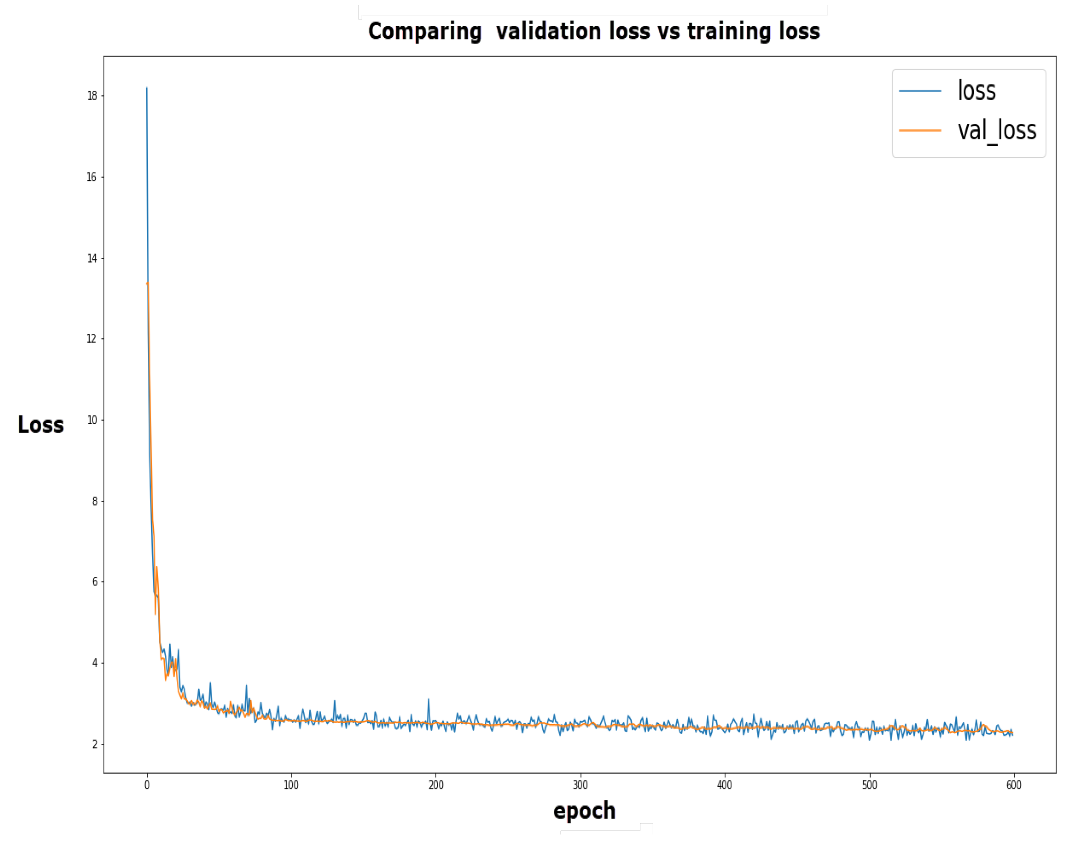
| Epochs | Val loss | ACC (%) | Conf (mAP) |
|---|---|---|---|
| 20 | 3.5099 | 49.5 | 0.5119 |
| 60 | 2.5054 | 82.5 | 0.4949 |
| 200 | 1.9740 | 99.5 | 0.6699 |
| 400 | 2.1127 | 97.1 | 0.5368 |
| 600 | 2.2741 | 95.5 | 0.5170 |
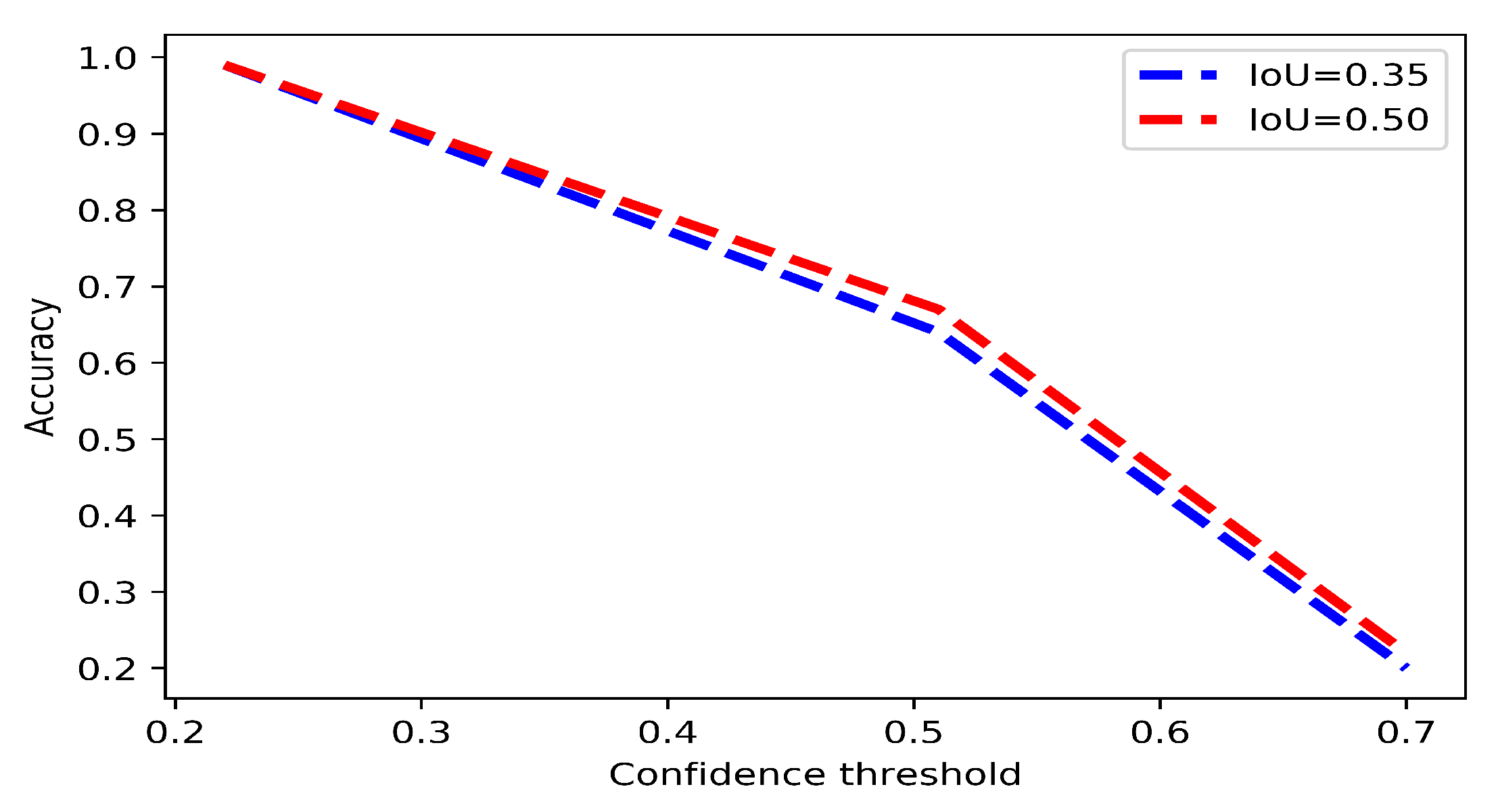
| Confidence Threshold | IoU | ACC (%) | PTPI(sec) | Conf(mAP) |
|---|---|---|---|---|
| 0.22 | 0.50 | 99.0 | 0.01450 | 0.5561 |
| 0.22 | 0.35 | 99.0 | 0.01316 | 0.5664 |
| 0.30 | 0.50 | 99.5 | 0.01500 | 0.6699 |
| 0.38 | 0.50 | 89.5 | 0.01599 | 0.5734 |
| 0.51 | 0.35 | 64.5 | 0.01453 | 0.6466 |
| 0.51 | 0.50 | 67.5 | 0.01479 | 0.6668 |
| 0.70 | 0.50 | 22.0 | 0.02250 | 0.7435 |
| 0.70 | 0.35 | 20.0 | 0.01710 | 0.7546 |
| Model Name | Database Size | Image Size | Epochs | val_loss | val_acc |
|---|---|---|---|---|---|
| DenseNet | 10,000 | (32, 32) | 10 | 0.1085 | 0.9912 |
| DenseNet | 1000 | (32, 32) | 10 | 0.7901 | 0.9421 |
| SqueezeNet | 1000 | (32, 32) | 10 | 0.6931 | 0.5000 |
| SqueezeNet | 1000 | (32,32) | 20 | 0.6931 | 0.5030 |
| SqueezeNet | 1000 | (32, 32) | 100 | 0.6931 | 0.5000 |
| SqueezeNet | 1000 | (64, 64) | 10 | 0.6931 | 0.4970 |
| SqueezeNet | 1000 | (480, 480) | 10 | 0.6931 | 0.5020 |
| ResNet50 | 1000 | (32, 32) | 10 | 0.2938 | 0.9268 |
| InceptionV3 | 1000 | (32, 32) | 10 | 0.1757 | 0.9573 |
| InceptionV3 | 1000 | (32, 32) | 100 | 0.2599 | 0.9360 |
| InceptionV3 | 1000 | (32, 32) | 50 | 0.1987 | 0.9543 |
| Method | Average Accuracy | ||
|---|---|---|---|
| Pearson’s correlation coefficient + Gabor Wavelet Transform [6] | 68.25 | 50 | 73.26% |
| Proposed (Densnet + SSD7) | 68.25 | 68.22 | 99.05% |
© 2020 by the authors. Licensee MDPI, Basel, Switzerland. This article is an open access article distributed under the terms and conditions of the Creative Commons Attribution (CC BY) license (http://creativecommons.org/licenses/by/4.0/).
Share and Cite
Bahaghighat, M.; Xin, Q.; Motamedi, S.A.; Zanjireh, M.M.; Vacavant, A. Estimation of Wind Turbine Angular Velocity Remotely Found on Video Mining and Convolutional Neural Network. Appl. Sci. 2020, 10, 3544. https://doi.org/10.3390/app10103544
Bahaghighat M, Xin Q, Motamedi SA, Zanjireh MM, Vacavant A. Estimation of Wind Turbine Angular Velocity Remotely Found on Video Mining and Convolutional Neural Network. Applied Sciences. 2020; 10(10):3544. https://doi.org/10.3390/app10103544
Chicago/Turabian StyleBahaghighat, Mahdi, Qin Xin, Seyed Ahmad Motamedi, Morteza Mohammadi Zanjireh, and Antoine Vacavant. 2020. "Estimation of Wind Turbine Angular Velocity Remotely Found on Video Mining and Convolutional Neural Network" Applied Sciences 10, no. 10: 3544. https://doi.org/10.3390/app10103544