Semi-Supervised Speech Recognition Acoustic Model Training Using Policy Gradient

Abstract

In this paper, we propose a policy gradient-based semi-supervised speech recognition acoustic model training. In practice, self-training and teacher/student learning are one of the widely used semi-supervised training methods due to their scalability and effectiveness. These methods are based on generating pseudo labels for unlabeled samples using a pre-trained model and selecting reliable samples using confidence measure. However, there are some considerations in this approach. The generated pseudo labels can be biased depending on which pre-trained model is used, and the training process can be complicated because the confidence measure is usually carried out in post-processing using external knowledge. Therefore, to address these issues, we propose a policy gradient method-based approach. Policy gradient is a reinforcement learning algorithm to find an optimal behavior strategy for an agent to obtain optimal rewards. The policy gradient-based approach provides a framework for exploring unlabeled data as well as exploiting labeled data, and it also provides a way to incorporate external knowledge in the same training cycle. The proposed approach was evaluated on an in-house non-native Korean recognition domain. The experimental results show that the method is effective in semi-supervised acoustic model training.

1. Introduction

Deep neural network (DNN)-based acoustic modeling has resulted in significant improvements in automatic speech recognition. For example, feed-forward deep neural network (FFDNN)-based acoustic models have achieved more improvement compared to Gaussian mixture model (GMM)-based acoustic models for phone-call transcription benchmark domains [1], and deep convolutional neural network (CNN)-based acoustic models outperformed FFDNNs on a news broadcast and switchboard task domains [2]. Recently, long short-term memory (LSTM)-based acoustic models have been reported to be more effective than FFDNNs or CNNs [3]. Although DNN-based acoustic modeling is successful, it requires a large amount of human labeled data to train acoustic models robustly. However, it is an expensive and time consuming job to collect a large amount of human labeled data considering various conditions, such as speakers, accents, channels, and multiple languages [4].

To handle the shortage of human labeled data, semi-supervised acoustic model training research has been conducted to use unlabeled data. The most representative approaches are graph-based learning, multi-task learning, self-training, and teacher/student learning. Graph-based learning focuses on jointly modeling labeled and unlabeled data as a weighted graph whose nodes represent data samples and whose edge weights represent pairwise similarities between samples [5,6]. The multi-task learning-based approaches focus on linearly combining the supervised cost with the unsupervised cost [7,8]. Self-training-based methods focus on generating machine transcriptions for unlabeled data using a pre-trained automatic speech recognition system and confidence measures, where confidence scores are computed with a forward–backward algorithm for a generated word lattice [9], or confusion networks [10,11]. Teacher/student learning-based approaches use the output distribution of the pre-trained model as a target for the student model to alleviate the complexity of confidence measures for large scale training [12].

Of these methods, self-training and teacher/student learning-based methods are widely used in practice due to their scalability and effectiveness [13,14,15]. However, there are some considerations regarding these methods. The accuracy of generated pseudo labels is affected by the performance of a pre-trained model, and there may even be no pre-trained model in the case of low-resource domains. In addition, the complexity of the training can increase because confidence measures, such as word lattice re-scoring, are usually carried out in post-processing. To alleviate the complexity issue, teacher/student learning-based methods use the posterior of the teacher model as a target distribution, but this method is a little complicated for incorporating external knowledge.

To handle these issues, we propose policy gradient method-based semi-supervised acoustic model training. The policy gradient method provides a straightforward framework that exploits labeled data, explores unlabeled data, and incorporates external knowledge in the same training cycle.

The rest of this paper is organized as follows. In Section 2, we briefly describe statistical speech recognition using a DNN-based acoustic model. Section 3 describes conventional semi-supervised acoustic model training methods. Section 4 presents our proposed approach in detail. Section 5 explains the experimental setting, and Section 6 presents the experimental results. Section 7 concludes the paper and discusses future work.

2. Statistical Speech Recognition Using a DNN-Based Acoustic Model

In this section, we briefly describe statistical speech recognition using a DNN-based acoustic model.

2.1. Statistical Speech Recognition

Statistical speech recognition is a process which finds a word sequence ${\mathbf{W}}^{*}$ that produces the highest probability for a given acoustic feature vector sequence $\mathbf{X}={\mathbf{x}}_1,{\mathbf{x}}_2,\dots ,{\mathbf{x}}_T$ as follows [16,17]:

$${\mathbf{W}}^{*}\approx argma{x}_{\mathbf{W}}P\left(\mathbf{W}\right|\mathbf{X})$$

(1)

In practice, it is divided into the following components by applying Bayes’ rule:

$$\begin{array}{cc}\hfill argma{x}_{\mathbf{W}}P\left(\mathbf{W}\right|\mathbf{X})& =argma{x}_{\mathbf{W}}\frac{P\left(\mathbf{X}\right|\mathbf{W})P\left(\mathbf{W}\right)}{P\left(\mathbf{X}\right)}\hfill \\ \hfill & =argma{x}_{\mathbf{W}}P\left(\mathbf{X}\right|\mathbf{W})P\left(\mathbf{W}\right)\hfill \end{array}$$

(2)

where $P\left(\mathbf{X}\right)$ is removed in recognition stage because the $argmax$ operator does not depend on $\mathbf{X}$. It is hard to model $P\left(\mathbf{X}\right|\mathbf{W})$ directly. So, words are represented by subword units $\mathbf{Q}$ [18]

$$\begin{array}{cc}\hfill argma{x}_{\mathbf{W}}P\left(\mathbf{X}\right|\mathbf{W})P\left(\mathbf{W}\right)& =argma{x}_{\mathbf{W}}\sum _{\mathbf{Q}}P\left(\mathbf{X}\right|\mathbf{Q},\mathbf{W})P(\mathbf{Q},\mathbf{W})\hfill \\ \hfill & \approx argma{x}_{\mathbf{W}}\sum _{\mathbf{Q}}P\left(\mathbf{X}\right|\mathbf{Q})P\left(\mathbf{Q}\right|\mathbf{W})P\left(\mathbf{W}\right)\hfill \\ \hfill & \approx argma{x}_{\mathbf{W}}ma{x}_{\mathbf{Q}}P\left(\mathbf{X}\right|\mathbf{Q})P\left(\mathbf{Q}\right|\mathbf{W})P\left(\mathbf{W}\right)\hfill \end{array}$$

(3)

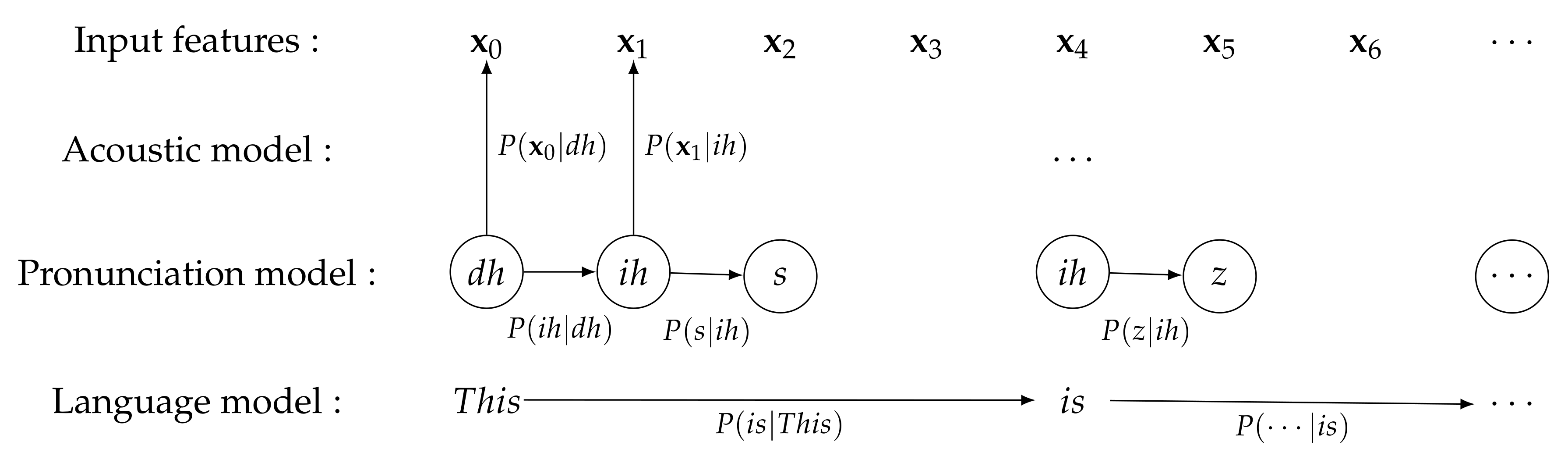
where $P\left(\mathbf{W}\right)$ is a language model, $P\left(\mathbf{Q}\right|\mathbf{W})$ is a pronunciation model and $P\left(\mathbf{X}\right|\mathbf{Q})$ is an acoustic model. Figure 1 depicts the role of the probabilistic models for ASR systems to recognize a given sentence “This is ⋯”. A language model, $P\left(\mathbf{W}\right)$, represents a priori probability of a word sequence. N-gram language model is commonly used by assuming that the word sequence depends only on the previous $N-1$ words. Figure 1 shows a 2-gram example. A pronunciation model, $P\left(\mathbf{Q}\right|\mathbf{W})$, plays a role to map words to their corresponding pronunciation or subword units. Figure 1 shows that the words, “This” and “is”, are mapped to phoneme sequence “dh ih s”, and “ih z” respectively. An acoustic model, $P\left(\mathbf{X}\right|\mathbf{Q})$, represents the probabilistic relationship between an input acoustic feature and the phonemes or other subword units.

Among these probabilistic models, we focus on acoustic model, especially training in a semi-supervised manner.

2.2. BLSTM-Based Acoustic Model

Various probabilistic models have been used for the acoustic model. In this study, we use bidirectional long short-term memory (BLSTM) for the acoustic model. For a given input feature sequence $\mathbf{X}={\mathbf{x}}_1,\cdots ,{\mathbf{x}}_T$, LSTM computes hidden vector at time, ${\mathbf{h}}_t$, using the function $\mathcal{H}({\mathbf{x}}_t,{\mathbf{h}}_{t-1},{\mathbf{c}}_{t-1})$ as follows [19,20,21]:

$$\begin{array}{c}{\mathbf{i}}_t=\sigma ({\mathbf{W}}_{xi}{\mathbf{x}}_t+{\mathbf{W}}_{hi}{\mathbf{h}}_{t-1}+{\mathbf{b}}_i)\hfill \end{array}$$

(4)

$$\begin{array}{c}{\mathbf{f}}_t=\sigma ({\mathbf{W}}_{xf}{\mathbf{x}}_t+{\mathbf{W}}_{hf}{\mathbf{h}}_{t-1}+{\mathbf{b}}_f)\hfill \end{array}$$

(5)

$$\begin{array}{c}{\mathbf{a}}_t=tanh({\mathbf{W}}_{xc}{\mathbf{x}}_t+{\mathbf{W}}_{hc}{\mathbf{h}}_{t-1}+{\mathbf{b}}_c)\hfill \end{array}$$

(6)

$$\begin{array}{c}{\mathbf{c}}_t={\mathbf{f}}_t\odot {\mathbf{c}}_{t-1}+{\mathbf{i}}_t\odot {\mathbf{a}}_t\hfill \end{array}$$

(7)

$$\begin{array}{c}{\mathbf{o}}_t=\sigma ({\mathbf{W}}_{xo}{\mathbf{x}}_t+{\mathbf{W}}_{ho}{\mathbf{h}}_{t-1}+{\mathbf{b}}_o)\hfill \end{array}$$

(8)

$$\begin{array}{c}\hfill {\mathbf{h}}_t={\mathbf{o}}_t\odot tanh\left({\mathbf{c}}_t\right)\end{array}$$

(9)

where the $\mathbf{W}$ means weight matrices, the $\mathbf{b}$ means bias vectors, $\sigma$ is the sigmoid function, $\mathbf{i}$, $\mathbf{f}$, $\mathbf{o}$ and $\mathbf{c}$ are respectively the input gate’s activation vector, forget gate’s activation vector, output gate’s activation vector and cell activation vector. BLSTM computes the forward hidden vector ${\overrightarrow{\mathbf{h}}}_t$, and the backward hidden vector ${\overleftarrow{\mathbf{h}}}_t$ at time t as follows [20]:

$${\overrightarrow{\mathbf{h}}}_t=\mathcal{H}({\mathbf{x}}_t,{\overrightarrow{\mathbf{h}}}_{t-1},{\overrightarrow{\mathbf{c}}}_{t-1})$$

(10)

$${\overleftarrow{\mathbf{h}}}_t=\mathcal{H}({\mathbf{x}}_t,{\overleftarrow{\mathbf{h}}}_{t+1},{\overleftarrow{\mathbf{c}}}_{t+1})$$

(11)

Then, the output is computed as follows [20]:

$${\mathbf{y}}_t={\mathbf{W}}_{\overrightarrow{h}y}{\overrightarrow{\mathbf{h}}}_t+{\mathbf{W}}_{\overleftarrow{h}y}{\overleftarrow{\mathbf{h}}}_t+{\mathbf{b}}_y$$

(12)

On top of the last layer, $softmax$ function is used to obtain the probability of the kth class for an input feature vector ${\mathbf{x}}_t$. For given input feature and target output dataset, $(\mathbf{X},\mathbf{Y})$, the BLSTM model parameter training is a general optimization problem to find parameters $\widehat{\theta }$ that minimizes a loss function, $\mathcal{J}(\mathbf{X},\mathbf{Y};\theta )$, as follows:

$$\widehat{\theta }=\underset{\theta }{argmin}\mathcal{J}(\mathbf{X},\mathbf{Y};\theta )$$

(13)

where the $\mathrm{argmin}$ operation is carried out through gradient descent algorithm as follows:

$${\theta }_{t+1}={\theta }_t-{\alpha }_t\nabla \mathcal{J}(\mathbf{X},\mathbf{Y};{\theta }_t)$$

(14)

where ${\alpha }_t$ is a learning rate.

3. Related Work

In this section, we describe semi-supervised acoustic model training for speech recognition in terms of a cross entropy loss minimization problem, and review how conventional methods obtain gradients $\nabla \mathcal{J}(\mathbf{X},\mathbf{Y};\theta )$ to update the model parameters. In particular, we focus on reviewing the self-training and teacher/student learning methods because they are most related to the proposed method.

3.1. Cross Entropy Loss

Semi-supervised acoustic model training can be formulated in terms of a cross entropy loss minimization problem for a given L number of labeled data $({\mathbf{X}}_l,{\mathbf{Y}}_l)={\left\{({\mathbf{x}}_i,y_i)\right\}}_1^L$ and U number of unlabeled data ${\mathbf{X}}_u={\left\{{\mathbf{x}}_{L+i}\right\}}_1^U$ as follows:

$$\mathcal{J}\left(\theta \right)=\frac{1}{L+U}\sum _{i=1}^{L+U}{\mathcal{J}}_i\left(\theta \right)$$

(15)

Here, the cross entropy loss ${\mathcal{J}}_i\left(\theta \right)$ measures the difference in probability distributions between the predicted labels and the ground truth labels for the ith input feature ${\mathbf{x}}_i$ as follows:

$${\mathcal{J}}_i\left(\theta \right)=-\sum _{k=1}^C{t}_k\left(y_i\right)log{P}_{\theta }(y_i=k|{\mathbf{x}}_i)$$

where C is the number of classes or output states, $t_k\left(y_i\right)$ is the distribution of the ground truth labels $y_i$, and $P_{\theta }(y_i=k|{\mathbf{x}}_i)$ is the distribution of the predicted labels.

3.2. Gradient of the Labeled Data

For the case of labeled data $({\mathbf{x}}_i,y_i)\in ({\mathbf{X}}_l,{\mathbf{Y}}_l)$, the distribution of the ground truth labels $t_k\left(y_i\right)$ is given in the form of one-hot encoding, such that the gradient for the ith labeled data is defined as

$$\nabla {\mathcal{J}}_i\left(\theta \right)=-\nabla log{P}_{\theta }(y_i=k|{\mathbf{x}}_i)$$

(16)

3.3. Gradient of the Unlabeled Data

For the case of unlabeled data ${\mathbf{x}}_i\in {\mathbf{X}}_u$, the ground truth distributions $t_k\left(y_i\right)$ are not given, so it is impossible to obtain the gradient of the cross entropy loss, $\nabla {\mathcal{J}}_i\left(\theta \right)$. To deal with this problem, self-training and teacher/student learning-based methods generate a pseudo ground truth distribution using a pre-trained model. 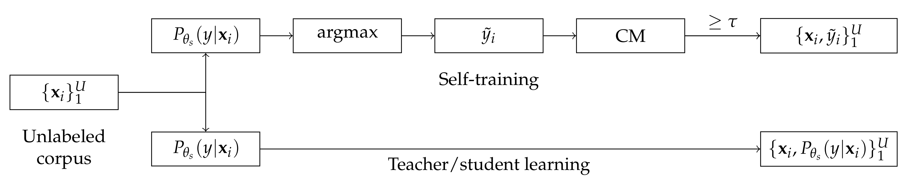Figure 2 shows the pseudo label generation process of self-training and teacher/student learning using a pre-trained model, $P_{{\theta }_s}\left(y\right|{\mathbf{x}}_i)$.

As shown in Figure 2, self-training-based approach generates a label, ${\tilde{y}}_i$, which produces the maximum posterior probability from a pre-trained model $\theta$ for an unlabeled input feature ${\mathbf{x}}_i$, and it is taken as a pseudo ground truth label, as follows [13,14,15]:

$${\tilde{y}}_i=argmax{P}_{\theta }(y_i=k|{\mathbf{x}}_i)$$

(17)

A confidence measure is then carried out to decide whether the sample is to be selected or not. Finally, the gradient of the unlabeled data can be obtained as follows:

$$\nabla {\mathcal{J}}_i\left(\theta \right)=\left\{\begin{array}{c}-\nabla log{P}_{\theta }\left({\tilde{y}}_i\right|{\mathbf{x}}_i),{\mathrm{CM}}_{\theta }\left({\tilde{y}}_i\right)\ge \gamma \hfill \\ 0.0,{\mathrm{CM}}_{\theta }\left({\tilde{y}}_i\right)<\gamma \hfill \end{array}\right.$$

(18)

where ${\mathrm{CM}}_{\theta }\left({\tilde{y}}_i\right)$ is the confidence measure and $\gamma$ is a threshold [22]. In some cases, normalized ${\mathrm{CM}}_{\theta }\left({\tilde{y}}_i\right)$ can be used for the pseudo ground truth distribution as follows:

$$\nabla {\mathcal{J}}_i\left(\theta \right)=-{\mathrm{CM}}_{\theta }\left({\tilde{y}}_i\right)\nabla log{P}_{\theta }\left({\tilde{y}}_i\right|{\mathbf{x}}_i)$$

(19)

However, the confidence measure is usually carried out as post-processing using external knowledge, such as language model, so it can increase the complexity of the semi-supervised learning. To alleviate the complexity of the confidence measure in the self-training methods, the teacher/student learning methods use the output distribution of a pre-trained model as a pseudo ground truth distribution $t_k\left(y_i\right)$, as follows [12]:

$$t_k\left({\tilde{y}}_i\right)=P_{\theta }({\tilde{y}}_i=k|{\mathbf{x}}_i)$$

(20)

So, the gradient of the unlabeled data can be obtained from

$$\nabla {\mathcal{J}}_i\left(\theta \right)=-\sum _{k=1}^c{t}_k\left({\tilde{y}}_i\right)\nabla log{P}_{\theta }({\tilde{y}}_i=k|{\mathbf{x}}_i)$$

(21)

In some sense, teacher/student learning can be understood as top-n pseudo label selection, from the viewpoint of self-training.

3.4. Considerations on Low-Resource Domain

Although self-training and teacher/student learning-based methods are popular due to their simplicity and effectiveness [13,14,15], the performance improvement highly depends on the robustness of a pre-trained model because pseudo labels are generated as a result of decoding process. In other words, if the pre-model is trained to be biased due to lack of a labeled training corpus, all generated pseudo labels for unlabeled data will be biased and eventually will not contribute to improve the performance. So, in this work, we focus on developing a semi-supervised training method that relaxes the dependency on a pre-trained model.

4. Semi-Supervised Acoustic Model Training Using Policy Gradient

In this section, we briefly describe reinforcement learning (RL) and then show how self-training and teacher/student learning-based methods can be dealt with from the aspect of RL problem.

This work is motivated by RL based speech processing [23,24], and the fundamental idea of the proposed approach is to deal with the acoustic model from the aspect of a policy network.

4.1. Policy Gradient

In a RL setting, an agent interacts with the environment via its actions and receives a reward. This transitions the agent into a new state, so that it gives a sequence of states, actions, and rewards known as a trajectory, $\tau$ [25,26,27].

$$S_0,A_0,R_1,S_1,A_1,R_2,\dots$$

(22)

If the total reward for a given trajectory $\tau$ is represented as $r\left(\tau \right)$, a loss of a RL is defined as a negative expected reward as follows:

$$\mathcal{J}\left(\theta \right)=-{\mathbb{E}}_{{\pi }_{\theta }}\left[r\left(\tau \right)\right]$$

(23)

where $r\left(\tau \right)$ is a reward when following a policy ${\pi }_{\theta }$, which is a probability distribution of actions given the state

$${\pi }_{\theta }(A_t=a|S_t=s),\forall A_t\in \mathcal{A}\left(s\right),S_t\in \mathcal{S}$$

(24)

where $\mathcal{A}\left(s\right)$ is a set of actions at state s and $\mathcal{S}$ is a set of states. The model parameters can be optimized as a gradient descent as follows:

$${\theta }_{t+1}={\theta }_t-{\alpha }_t\nabla \mathcal{J}\left(\theta \right)$$

(25)

The gradient of the loss function $\nabla \mathcal{J}\left(\theta \right)$ can be derived using a log-trick as follows [25,27]:

$$\begin{array}{cc}\nabla \mathcal{J}\left(\theta \right)\hfill & =-\nabla \int {\pi }_{\theta }\left(\tau \right)r\left(\tau \right)d\tau \hfill \end{array}$$

(26)

$$\begin{array}{cc}\hfill & =-\int {\pi }_{\theta }\left(\tau \right)\nabla log{\pi }_{\theta }\left(\tau \right)r\left(\tau \right)d\tau \hfill \end{array}$$

(27)

$$\begin{array}{cc}\hfill & =-{\mathbb{E}}_{{\pi }_{\theta }}[r\left(\tau \right)\nabla log{\pi }_{\theta }\left(\tau \right)]\hfill \end{array}$$

(28)

Then, expanding the definition of ${\pi }_{\theta }\left(\tau \right)$,

$${\pi }_{\theta }\left(\tau \right)=P\left(s_0\right)\prod _{t=1}^T{\pi }_{\theta }\left(a_t\right|s_t)p(s_{t+1},r_{t+1}|s_t,a_t)$$

(29)

$$\nabla log{\pi }_{\theta }\left(\tau \right)=\sum _{t=1}^T\nabla log{\pi }_{\theta }\left(a_t\right|s_t)$$

(30)

Finally, the gradient can be defined as follows:

$$\nabla \mathcal{J}\left(\theta \right)={\mathbb{E}}_{{\pi }_{\theta }}[\sum _{t=1}^T\nabla {\mathcal{J}}_t\left(\theta \right)]$$

(31)

where

$$\nabla {\mathcal{J}}_t\left(\theta \right)=-G_t\nabla log{\pi }_{\theta }\left(a_t\right|{\mathbf{s}}_t)$$

(32)

4.2. Relation between Gradients of Cross Entropy Loss and Reward Loss

It should be noted that the gradients of cross entropy loss and expected reward can be considered virtually the same as weighted negative log likelihood as shown in Equations (19) and (32). This implies that the conventional methods can be dealt with from the aspect of policy gradient method. To deal with semi-supervised learning from the aspect of RL, action and reward must be defined and

Table 1. Semi-supervised learning from the aspect of policy gradient.

Type	${\mathit{s}}_{\mathit{t}}$	${\mathit{a}}_{\mathit{t}}$	${\mathit{G}}_{\mathit{t}}$
Labeled	${\mathbf{x}}_t$	$y_t$	$1.0$
Unlabeled	${\mathbf{x}}_t$	${\tilde{y}}_t\sim P_{\theta }(y_t=k|{\mathbf{x}}_t)$	$Q\left({\tilde{y}}_t\right)$

summarizes the difference between labeled data and unlabeled data. For the labeled data, action $a_t$ is the same as the ground truth label $y_t$, and reward $G_t$ is $1.0$ because the ground truth label $y_t$ is the action that we exactly expected. However, for the unlabeled data, action is sampled from the policy network instead of $argmax\left(\right)$, and reward $G_t$ for the action is assigned by a Q-function $Q\left({\tilde{y}}_t\right)$.

In the policy gradient method based approach, sampling-based pseudo label generation can reduce the excessive dependency of the pre-trained model, and the Q-function plays a role to regularize the model not to be skewed using external knowledge in the same training cycle.

4.3. Semi-Supervised Learning Using Policy Gradient

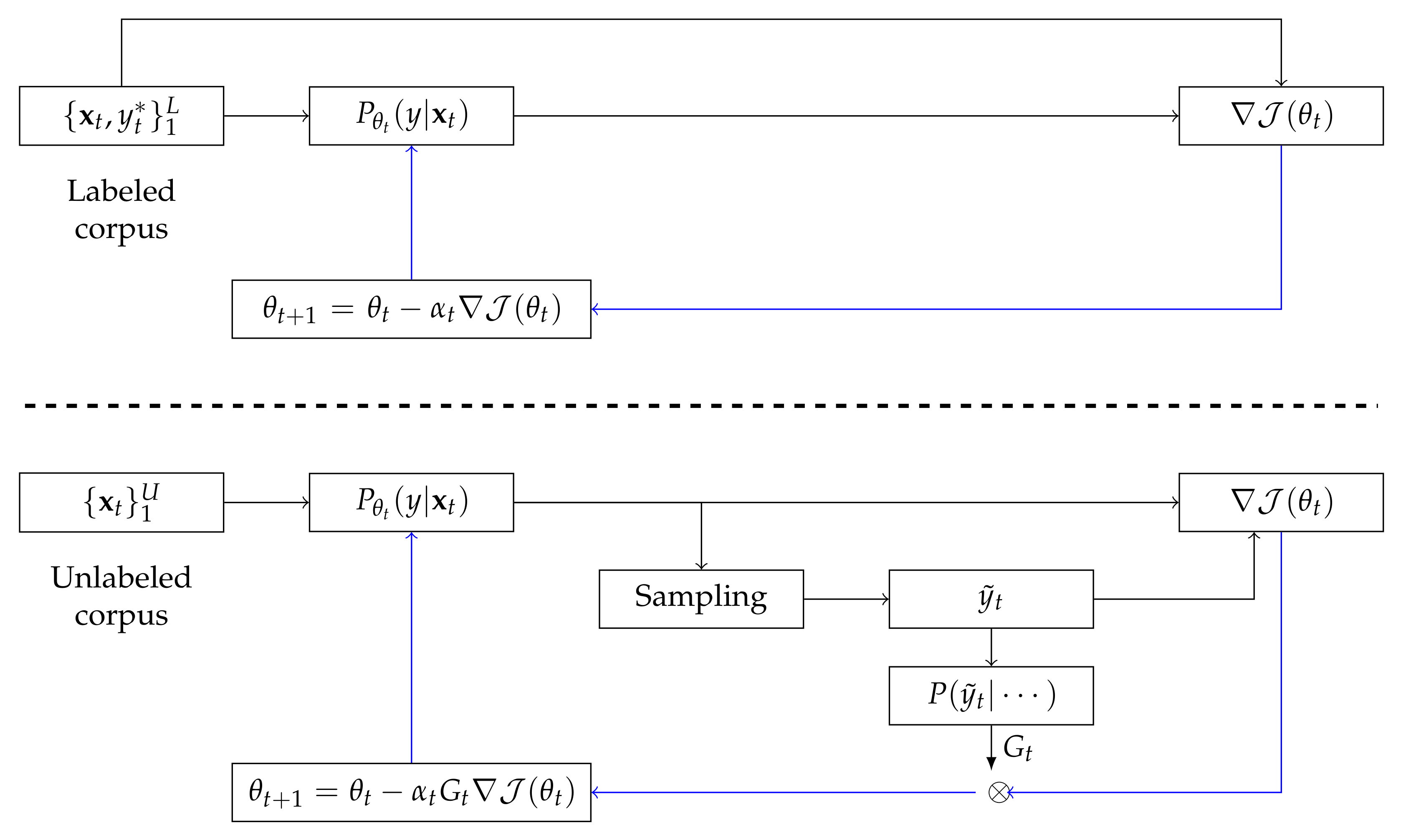
The proposed semi-supervised training consists of interleaved training and fine-tuning. Fine-tuning just performs one-epoch supervised training for the human-labeled data after finishing interleaved training. Figure 3. illustrates the proposed semi-supervised training procedure. For the labeled corpus, gradients of cross entropy loss between the ground truth labels and predictions are used to update model parameters. However, gradients of reward loss between sampled pseudo labels and predictions are used for unlabeled corpus.

Algorithm 1 describes the proposed training procedure in detail. In the algorithm, $I_u$ and $I_l$ are respectively the number of unlabeled and labeled data blocks composed of about one-hour speech data, and ${({\mathbf{X}}_l,{\mathbf{Y}}_l)}^i$ and ${\left({\mathbf{X}}_u\right)}^i$ indicates the ith block.

Algorithm 1 Proposed learning procedure

Require:   A training set $({\mathbf{X}}_l,{\mathbf{Y}}_l),\left({\mathbf{X}}_u\right)$, initial values ${\theta }_0$

1. Interleaved training

1: while not converged do 2:     for $i=1$ to $I_u$ do 3:         if $i\mathrm{mod}m==0$ then 4:            Select labeled data $({\mathbf{x}}_t,y_t)\in {({\mathbf{X}}_l,{\mathbf{Y}}_l)}^{i\%I_l}$ 5:            $a_t\leftarrow y_t$ 6:            $G_t\leftarrow 1.0$ 7:            ${\theta }_{t+1}\leftarrow {\theta }_t-{\alpha }_t{G}_t{\nabla }_{\theta }{P}_{\theta }\left(a_t\right|{\mathbf{x}}_t)$ 8:         end if 9:         Select unlabeled data ${\mathbf{x}}_t\in {\left({\mathbf{X}}_u\right)}^i$ 10:         $a_t\sim P_{\theta }(y_t=k|{\mathbf{x}}_t)$ 11:         $G_t\leftarrow Q\left(a_t\right)$ 12:         ${\theta }_{t+1}\leftarrow {\theta }_t-{\alpha }_t{G}_t{\nabla }_{\theta }{P}_{\theta }\left(a_t\right|{\mathbf{x}}_t)$ 13:     end for 14: end while

2. Fine-tuning

15: for$i=1$ to $I_l$ do 16:     Select a labeled data subset $({\mathbf{x}}_t,y_t)\in {({\mathbf{X}}_l,{\mathbf{Y}}_l)}^i$ 17:     $a_t\leftarrow y_t$ 18:     $G_t\leftarrow 1.0$ 19:     ${\theta }_{t+1}\leftarrow {\theta }_t-{\alpha }_t{G}_t{\nabla }_{\theta }{P}_{\theta }\left(a_t\right|{\mathbf{x}}_t)$ 20: end for

The proposed algorithm is affected by the following three parameters:

• Modulus m controls the interleaving rate. Human labeled data is used once every m iterations.
• Temperature T controls the reliability of generated pseudo labels when using temperatured-$softmax\left(\right)$, as follows [28]:

  $$P_{\theta }(y_t=k|{\mathbf{x}}_t)=\frac{exp(z_k/T)}{{\sum }_{j}exp(z_j/T)}$$

  (33)
• Q-function $Q\left({\tilde{y}}_t\right)$ is used to weight the sampled action $a_t$. Two types of Q-functions are investigated. One is a fixed reward that reflects relative reliability of single sampled action compared to the human labeled action, and the other is a state-level n-gram to consider reliability of the sampled action sequence, as follows:

  $$Q\left({\tilde{y}}_t\right)=\left\{\begin{array}{c}r\hfill \\ P\left({\tilde{y}}_t\right|{\tilde{y}}_{t-1}\dots )\hfill \end{array}\right.$$

  (34)

5. Experimental Setting

In this section, we describe the experimental setting in detail.

5.1. Non-Native Korean Database

The in-house non-native Korean corpus for Korean speaking education contains about 133 h of 123,617 sentences spoken by 417 non-native Korean speakers. The speech data were recorded at a rate of 16 kHz. All utterances were recorded so as not to have reading errors such as insertions or deletions. The non-native speakers were Asians from China, Japan, and Vietnam. The gender and spoken language proficiency levels were evenly distributed among the speaker. For the corpus, 13 h have been transcribed by humans and another 120 h are not labeled. For the labeled corpus, one hour of the training data was randomly held out without overlapping as part of the test set. Each 20 ms speech frame was represented by 40-dimensional Mel filter bank (MFB) features by using the Kaldi toolkit [29]. The 600-dimensional MFB features considering seven left and right contexts were used to represent each frame. For distributed BLSTM training, one iteration of data is composed of about one-hour of speech data. So, the numbers of labeled, $I_l$, and unlabeled data, $I_u$, are 12 and 120, respectively.

5.2. Alignment for the Human Labeled Corpus

A Gaussian Mixture Model-hidden Markov model (GMM-HMM) acoustic model was trained using the Kaldi toolkit to generate a force-aligned transcription for labeled data. The GMM-HMM was built using the “s5” procedure provided by the Kaldi toolkit. For the forced-aligned transcriptions, physical GMM n-grams were obtained using KenLM toolkit [30].

5.3. BLSTM Training

The Pytorch toolkit was used to implement the proposed approach and to train the BLSTM model parameters [31]. the BLSTM was configured with 6 layers each with 320 units and a temperatured-$softmax\left(\right)$ with 2920 units corresponding to the physical GMMs. The training batch size was 30 and AdaDelta [32] optimization with an initial learning rate set to 1.0 is used. Any regularization nor dropout is not applied, and fifteen epochs of training were performed.

6. Experimental Results

In this experiment, we measured the performance of a supervised model and a self-trained model as a baseline system. The supervised model was trained using the 12-h human labeled data, and self-training model was trained by the conventional self-training method for the 120-h unlabeled data using the supervised model as a pre-trained model.

The performance was measured by frame accuracy, and

Table 2. Baseline performance.

Model	Frame Acc (%)
Supervised	52.03
Self-training	52.71

shows the results. As shown, there is a little improvement with self-training-based approach. However, it seems natural because about 48% of pseudo labels are expected to contain errors by the pre-trained model. So, optimizing for the erroneous pseudo labels is not expected to improve the performance.

Table 3. The proposed method performance.

	m	T	$\mathbf{Q}\left({\mathbf{a}}_{\mathbf{t}}\right)$	Frame Acc (%)
Modulus	3	1.0	1.0	54.12
	2	1.0	1.0	54.58
	1	1.0	1.0	54.62
Temperature	1	0.9	1.0	55.42
	1	0.8	1.0	55.56
	1	0.7	1.0	55.47
	1	0.6	1.0	55.36
Q-function	1	0.8	0.9	55.62
	1	0.8	0.8	56.11
	1	0.8	0.7	55.81
	1	0.8	3-gram	57.11
	1	0.8	5-gram	57.31
	1	0.8	10-gram	57.22

shows the performance of the proposed method. The hyper parameters such as, modulus m, temperature T, and Q-function $Q\left(a_t\right)$, are tuned sequentially. For the different three modulus m, the best performance is obtained by training labeled data and unlabeled data interleavely by setting m as 1. However, there is little accuracy degradation even if labeled data was used once every in 3 iterations. Temperature, T, controls the randomness of pseudo label generation. The smaller the value, the same as using $argmax\left(\right)$, and the same as selecting randomly at large. In this experiment, there is a slight improvement by setting T as smaller than $1.0$. It implies that sampling-based pseudo label generation gives more chance to explore correct generation than $argmax\left(\right)$. Q-function, $Q\left(a_t\right)$, plays role to weight the reliability of sampled pseudo label. Assuming that the reliability of human labels is $1.0$, it may be reasonable that the reliability of pseudo labels is lower than $1.0$. In this case, $0.8$ shows the best accuracy for the case of constant value. For the case of considering temporal reliability using n-gram. In this case, 5-gram shows the best performance.

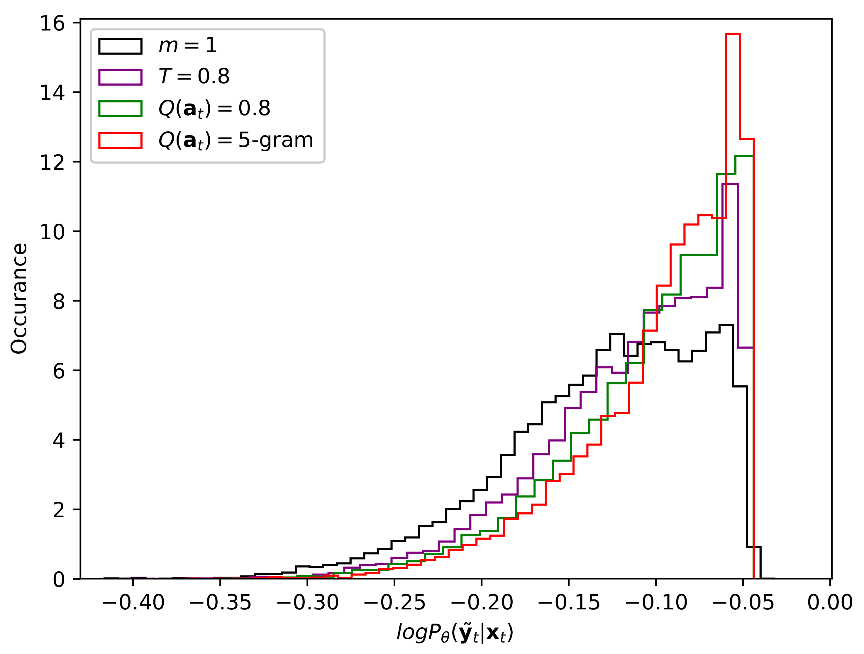
In general, entropy minimization is considered in the semi-supervised training-based on the assumption that classifier’s decision boundary should not pass through high-density regions of the marginal data distribution [33,34]. Figure 4 shows the histogram of $log{P}_{\theta }\left(\tilde{\mathbf{y}}\right|\mathbf{x})$ of unlabeled data in this experiment. It shows that the model’s predictions become more confident or entropy decreases by tuning the hyper-parameters. It implies that the proposed method is effective for semi-supervised training for acoustic model.

7. Conclusions

Although self-training or teacher/student learning-based semi-supervised acoustic model training methods are among the most popular approaches, these methods are not effective if a pre-trained model is not matched to unlabeled data or there is no pre-trained model.

To deal with the problem, we proposed a policy gradient method-based semi-supervised acoustic model training method. The proposed method provides a straightforward framework for exploring unlabeled data as well as exploiting the pre-trained model, and it also provides a way to incorporate various external knowledge in the same training cycle. The experimental results show that the proposed method outperforms the conventional self-training method because the proposed method provides a way to balance exploiting the pre-trained model and exploring unlabeled data, and to weight pseudo labels according to static or temporal reliability.

In our future work, we are plan to use end-to-end speech recognition framework for more sophisticate modeling, and investigate more reward functions, and also apply advanced techniques developed in RL-based learning.

References

- Seide, F.; Li, G.; Yu, D. Conversational speech transcription using context-dependent deep neural networks. In Proceedings of the Twelfth Annual Conference of the International Speech Communication Association, Florence, Italy, 27–31 August 2011. [Google Scholar]
- Sainath, T.N.; Mohamed, A.r.; Kingsbury, B.; Ramabhadran, B. Deep convolutional neural networks for LVCSR. In Proceedings of the 2013 IEEE International Conference on Acoustics, Speech and Signal Processing, Vancouver, BC, Canada, 26–31 May 2013; pp. 8614–8618. [Google Scholar]
- Sak, H.; Senior, A.; Beaufays, F. Long short-term memory recurrent neural network architectures for large scale acoustic modeling. In Proceedings of the Fifteenth Annual Conference of the International Speech Communication Association, Singapore, 14–18 September 2014. [Google Scholar]
- Liu, Y.; Kirchhoff, K.; Liu, Y.; Kirchhoff, K. Graph-based semisupervised learning for acoustic modeling in automatic speech recognition. IEEE/ACM Trans. Audio Speech Lang. Process. (TASLP) 2016, 24, 1946–1956. [Google Scholar] [CrossRef]
- Liu, Y.; Kirchhoff, K. Graph-based semi-supervised learning for phone and segment classification. In Proceedings of the INTERSPEECH 2013—14th Annual Conference of the International Speech Communication Association, Lyon, France, 25–29 August 2013; pp. 1840–1843. [Google Scholar]
- Liu, Y.; Kirchhoff, K. Graph-based semi-supervised acoustic modeling in DNN-based speech recognition. In Proceedings of the 2014 IEEE Spoken Language Technology Workshop (SLT), South Lake Tahoe, NV, USA, 7–10 December 2014; pp. 177–182. [Google Scholar]
- Ranzato, M.; Szummer, M. Semi-supervised learning of compact document representations with deep networks. In Proceedings of the 25th International Conference on Machine Learning, Helsinki, Finland, 5–9 July 2008; pp. 792–799. [Google Scholar]
- Dhaka, A.K.; Salvi, G. Sparse autoencoder based semi-supervised learning for phone classification with limited annotations. In Proceedings of the GLU 2017 International Workshop on Grounding Language Understanding, Stockholm, Sweden, 25 August 2017; pp. 22–26. [Google Scholar]
- Wessel, F.; Ney, H. Unsupervised training of acoustic models for large vocabulary continuous speech recognition. IEEE Trans. Speech Audio Process. 2005, 13, 23–31. [Google Scholar] [CrossRef]
- Wang, L.; Gales, M.J.; Woodland, P.C. Unsupervised training for Mandarin broadcast news and conversation transcription. In Proceedings of the 2007 IEEE International Conference on Acoustics, Speech and Signal Processing-ICASSP’07, Honolulu, HI, USA, 15–20 April 2007; Volume 4, pp. 353–356. [Google Scholar]
- Yu, K.; Gales, M.; Wang, L.; Woodland, P.C. Unsupervised training and directed manual transcription for LVCSR. Speech Commun. 2010, 52, 652–663. [Google Scholar] [CrossRef]
- Parthasarathi, S.H.K.; Strom, N. Lessons from building acoustic models with a million hours of speech. In Proceedings of the ICASSP 2019—2019 IEEE International Conference on Acoustics, Speech and Signal Processing (ICASSP), Brighton, UK, 12–17 May 2019; pp. 6670–6674. [Google Scholar]
- Liao, H.; McDermott, E.; Senior, A. Large scale deep neural network acoustic modeling with semi-supervised training data for YouTube video transcription. In Proceedings of the 2013 IEEE Workshop on Automatic Speech Recognition and Understanding, Olomouc, Czech Republic, 8–12 December 2013; pp. 368–373. [Google Scholar]
- Huang, Y.; Yu, D.; Gong, Y.; Liu, C. Semi-supervised GMM and DNN acoustic model training with multi-system combination and confidence re-calibration. In Proceedings of the INTERSPEECH 2013—14th Annual Conference of the International Speech Communication Association, Lyon, France, 25–29 August 2013; pp. 2360–2364. [Google Scholar]
- Huang, Y.; Wang, Y.; Gong, Y. Semi-Supervised Training in Deep Learning Acoustic Model. In Proceedings of the INTERSPEECH 2016—17th Annual Conference of the International Speech Communication Association, San Francisco, CA, USA, 8–12 September 2016; pp. 3848–3852. [Google Scholar]
- Jelinek, F. Continuous speech recognition by statistical methods. Proc. IEEE 1976, 64, 532–556. [Google Scholar] [CrossRef]
- Jelinek, F. Statistical Methods for Speech Recognition; MIT Press: Cambridge, MA, USA, 1997. [Google Scholar]
- Fosler-Lussier, J.E. Dynamic Pronunciation Models for Automatic Speech Recognition. Ph.D. Thesis, University of California, Berkeley Fall, CA, USA, 1999. [Google Scholar]
- Graves, A.; Fernández, S.; Schmidhuber, J. Bidirectional LSTM networks for improved phoneme classification and recognition. In Proceedings of the ICANN 2005—International Conference on Artificial Neural Networks, Warsaw, Poland, 11–15 September 2005; pp. 799–804. [Google Scholar]
- Graves, A.; Jaitly, N.; Mohamed, A.-r. Hybrid speech recognition with deep bidirectional LSTM. In Proceedings of the 2013 IEEE Workshop on Automatic Speech Recognition and Understanding, Olomouc, Czech Republic, 8–12 December 2013; pp. 273–278. [Google Scholar]
- Zeyer, A.; Doetsch, P.; Voigtlaender, P.; Schlüter, R.; Ney, H. A comprehensive study of deep bidirectional LSTM RNNs for acoustic modeling in speech recognition. In Proceedings of the 2017 IEEE International Conference on Acoustics, Speech and Signal Processing (ICASSP), New Orleans, LA, USA, 5–9 March 2017; pp. 2462–2466. [Google Scholar]
- Jiang, H. Confidence measures for speech recognition: A survey. Speech Commun. 2005, 45, 455–470. [Google Scholar] [CrossRef]
- Kala, T.; Shinozaki, T. Reinforcement learning of speech recognition system based on policy gradient and hypothesis selection. In Proceedings of the 2018 IEEE International Conference on Acoustics, Speech and Signal Processing (ICASSP), Calgary, AB, Canada, 15–20 April 2018; pp. 5759–5763. [Google Scholar]
- Zhou, Y.; Xiong, C.; Socher, R. Improving end-to-end speech recognition with policy learning. In Proceedings of the 2018 IEEE International Conference on Acoustics, Speech and Signal Processing (ICASSP), Calgary, AB, Canada, 15–20 April 2018; pp. 5819–5823. [Google Scholar]
- Kaelbling, L.P.; Littman, M.L.; Moore, A.W. Reinforcement learning: A survey. J. Artif. Intell. Res. 1996, 4, 237–285. [Google Scholar] [CrossRef]
- Sutton, R.S.; Barto, A.G. Reinforcement Learning: An Introduction; MIT Press: Cambridge, MA, USA, 2018. [Google Scholar]
- Sutton, R.S.; McAllester, D.A.; Singh, S.P.; Mansour, Y. Policy gradient methods for reinforcement learning with function approximation. In Advances in Neural Information Processing Systems; NIPS: San Diego, CA, USA, 2000; pp. 1057–1063. [Google Scholar]
- Hinton, G.; Vinyals, O.; Dean, J. Distilling the knowledge in a neural network. arXiv 2015, arXiv:1503.02531. [Google Scholar]
- Povey, D.; Ghoshal, A.; Boulianne, G.; Burget, L.; Glembek, O.; Goel, N.; Hannemann, M.; Motlicek, P.; Qian, Y.; Schwarz, P.; et al. The Kaldi speech recognition toolkit. In Proceedings of the IEEE 2011 Workshop on Automatic Speech Recognition and Understanding, Waikoloa, HI, USA, 11–15 December 2011. number EPFL-CONF-192584. [Google Scholar]
- Heafield, K. KenLM: Faster and smaller language model queries. In Proceedings of the Sixth Workshop on Statistical Machine Translation, Edinburgh, UK, 30–31 July 2011; pp. 187–197. [Google Scholar]
- Paszke, A.; Gross, S.; Chintala, S.; Chanan, G.; Yang, E.; DeVito, Z.; Lin, Z.; Desmaison, A.; Antiga, L.; Lerer, A. Automatic Differentiation in PyTorch. In Proceedings of the NIPS Autodiff Workshop, Long Beach, CA, USA, 9 December 2017. [Google Scholar]
- Zeiler, M.D. ADADELTA: An adaptive learning rate method. arXiv 2012, arXiv:1212.5701. [Google Scholar]
- Grandvalet, Y.; Bengio, Y. Semi-supervised learning by entropy minimization. In Proceedings of the NIPS 2005—Advances in Neural Information Processing Systems, Vancouver, BC, Canada, 5–8 December 2005; pp. 529–536. [Google Scholar]
- Berthelot, D.; Carlini, N.; Goodfellow, I.; Papernot, N.; Oliver, A.; Raffel, C.A. Mixmatch: A holistic approach to semi-supervised learning. In Proceedings of the NIPS 2019—Advances in Neural Information Processing Systems, Vancouver, BC, Canada, 8–14 December 2019; pp. 5050–5060. [Google Scholar]
© 2020 by the authors. Licensee MDPI, Basel, Switzerland. This article is an open access article distributed under the terms and conditions of the Creative Commons Attribution (CC BY) license (http://creativecommons.org/licenses/by/4.0/).