Article

A Hierarchical Control System for Autonomous Driving towards Urban Challenges

Intelligent Robotics Laboratory, Department of Control and Robot Engineering, Chungbuk National University, Cheongju-si 28644, Korea
*
Author to whom correspondence should be addressed.
Current Address: Chungdae-ro 1, Seowon-Gu, Cheongju, Chungbuk 28644, Korea.
Appl. Sci. 2020, 10(10), 3543; https://doi.org/10.3390/app10103543
Submission received: 23 April 2020 / Revised: 14 May 2020 / Accepted: 18 May 2020 / Published: 20 May 2020
(This article belongs to the Special Issue Intelligent Control and Robotics)

Abstract

:
In recent years, the self-driving car technologies have been developed with many successful stories in both academia and industry. The challenge for autonomous vehicles is the requirement of operating accurately and robustly in the urban environment. This paper focuses on how to efficiently solve the hierarchical control system of a self-driving car into practice. This technique is composed of decision making, local path planning and control. An ego vehicle is navigated by global path planning with the aid of a High Definition map. Firstly, we propose the decision making for motion planning by applying a two-stage Finite State Machine to manipulate mission planning and control states. Furthermore, we implement a real-time hybrid A* algorithm with an occupancy grid map to find an efficient route for obstacle avoidance. Secondly, the local path planning is conducted to generate a safe and comfortable trajectory in unstructured scenarios. Herein, we solve an optimization problem with nonlinear constraints to optimize the sum of jerks for a smooth drive. In addition, controllers are designed by using the pure pursuit algorithm and the scheduled feedforward PI controller for lateral and longitudinal direction, respectively. The experimental results show that the proposed framework can operate efficiently in the urban scenario.

1. Introduction

According to a survey reported in 2018 [1], the number of on-road accidents is more than 90% caused by personal inadvertences. Self Driving Cars (SDCs) are a prominent method for the human to solve collisions, frustrating situations, and decrease energy expenditure. Although SDCs have breakthroughs in trial stages, the governments are still hesitant to commercialize due to the worry about safety in public transport. Recently, SDCs technology has been developed with a large number of studies, especially in the epoch of deep learning. Besides, the biggest challenge of SDC technology is that it needs to handle all circumstances on the road like expert drivers.
Within 2016, the Society of Automotive Engineers (SAE) defined various criteria of the autonomy level of SDCs [2]. Firstly, it starts at level 0 with comprehensive human handling. Level 1 can support the driver by operating either lane-keeping assist systems or adaptive cruise control. Level 2, which assists human drivers in steering and acceleration control, operates similarly to level 1 but is more intelligent in specific driving scenarios. At level 3, the autonomous module can conduct perception tasks like object detection and tracking to intervene in the control tasks, this level requires frequent human override for vehicle control. At level 4, the operation can manage most of the circumstances on the road; nevertheless, human override is an option to handle unexpected scenarios. To the best of our knowledge, at this level, an exclusively self-driving company named Waymo is ready to deploy in public transportation over numerous million miles on city roads in fall 2018 [3]. Level 5 is designated to a fully autonomous vehicle.
The Defense Advanced Research Projects Agency (DARPA) started an autonomous driving challenge in 2002 [4]. This challenge can be considered as the first well-known experiment for SDCs, and it opened the imagination of humans about what the autonomous vehicle can do. The first competition was held and awarded one million dollars for the winner on March 13, 2004 [4]. However, in the first contest, no team could complete the challenge. The second DARPA grand challenge was held on October 8, 2005 [4]. Five teams of twenty-three could accomplish the autonomous driving mode. Stanley robot of Stanford won the competition followed by Sandstorm of Carnegie Mellon. Later, on November 3, 2007, the DARPA established a competition called DARPA Urban Challenge, which operated on busy roads and needed much more intelligent motion planning and perception [4,5]. This competition also required vehicles to drive automatically in several locations with GPS-denied environments. The winning team was Boss of Carnegie Mellon University, and the Stanford Junior team came second. After the DARPA competition, many autonomous vehicle challenges and tests have been organized. The European Land-Robot Trial (ELROB) [6] has been conducted from 2006 to the present. From 2009 to 2013, the Intelligent Vehicle Future Challenge in China was held [7]. In South Korea, the autonomous vehicle challenge was firstly announced by Hyundai cooperation in August 2008 [8]. The most recent competition was announced in March 2018 and organized in July 2019. The organizer built a testing ground called K-city to mimic the urban area.
From that time of the final DARPA Urban Challenge, many successful stories in the industry of autonomous driving in urban environments have been reported. Specifically, Google’s self-driving car had driven automatically over 140 thousand miles in California in 2010 [9]. About four years later, Google successfully developed an autonomous vehicle that can be driven up to 40 kilometers per hour in the urban area. In 2016, Google’s autonomous driving vehicle was renamed to Waymo [3]. From that moment, Waymo has been getting many achievements and leading the race to get autonomous cars into public transportation. Around the end of 2015, the Tesla company induced an autonomous driving vehicle called Autopilot to market [10]. In 2016, the Tesla Model S had a disastrous accident in Florida. The reason for this accident was the simultaneous failure of both camera and radar sensors. Despite suffering severe problems, the self-driving automobiles are continuously developed. Recently, Zoox and nuTonomy have led the autonomous taxi business. Numerous start-up businesses have been establishing and reinforced to bring safe autonomous vehicles to trade as early as 2020. Autoware [11], Apollo [12], NVIDIA DriveWorks [13] and Openpilot [14] are the most popular open-source frameworks. We highlight that Autoware [11] and Apollo [12] using the Robot Operating System (ROS) [15] that can be flexibly integrated into real-world applications.
Roughly speaking, the autonomous vehicle system can be commonly divided into three primary classes [16,17], including perception and environment mapping, motion planning and control system. In this article, we develop an autonomous driving system, as shown in Figure 1. The perception and environment mapping are applied to determine where the self-driving vehicle is and what surrounding environments are. One of the most challenging issues in the urban scene is less-texture and high illumination. So that the localization algorithm could achieve precision and be robust in the area, the localization uses the inertial navigation system (INS) with an Inertial Measurement Unit (IMU) and Global Positioning System (GPS) fusion to avoid drift over time [16,17]. In GPS-denied environments such as a tunnel scene, the 3D LiDAR odometry [18] technique is implemented to localize itself. The prediction uses the Interactive Multiple Model–Unscented Kalman Filter–Joint Probabilistic Data Association Filter (IMM-UKF-JPDAF) method [19], which predict the trajectories of the dynamic objects such as vehicles, pedestrian. The motion planning categorizes into three groups [16,17,20] global path planning (GPP), decision-making and local planning. The GPP makes route planning, which plots through a series of lanes or roads efficiently. The GPP generally uses a High Definition (HD) Map, which provides ad-hoc structured information regarding the streets and Vehicle-to-X (V2X) communication technology, then it chooses the best route via a series of waypoints.
This paper focuses on handling a hierarchical control system including decision making, local path planning and control. The decision-making can be divided into Finite State Machines (FSM) and Markov Decision Processes (MDPs) [16,17]. MDPs is useful for solutions with uncertainty information of perception and quite complicates to implement with a large variety of scenarios. In contrast, FSM is a simple method and handles well with many circumstances. In the DARPA Urban Challenge, Stanford Junior team succeeded in applying FSM with several scenarios in urban traffic roads [4]. However, the main drawback of FSM is the difficulty in solving uncertainty and in large-scale scenarios. In this work, we propose the decision-making with a new structure to manage various traffic scenarios and road conditions. This FSM contains the mission that the vehicle should perform and the behavior of the car, such as lane-changing, lane-keeping, obeying traffic lights, and rule-based speed limits. The local path planner (LPP) generates a regional trajectory for the autonomous vehicle in both structured and unstructured scenarios. Researchers in [21] used the decoupled approach of path and velocity to produce a speed profile, although this solution is not optimal but straightforward. Appolo [12] performs the spline path by determining a QP optimization problem with linearized constraints. Despite this algorithm is an effective method but not optimal with the temporal variable. In this paper, we solve the LPP by exploring an optimization problem in the Frenet coordinate [22]. Herein, we define the optimization problem with not only trajectory parameters but also travel time, and additionally join the constraints of input and output velocity. After solving this optimization problem, we have both spatial and temporal parameters for the control. Recently, the deep learning approaches can be employed to manage lateral control directly [23] or aid the controller [24]. Nevertheless, the computational cost, complexity, and less robustness are the main drawbacks of the method. The classical controller as the PID method is the most popular control strategy which operates adequately in various applications of process control. However, distributed noises such as road conditions, friction forces are hard to handle by the PID controller. Moreover, the Model Predictive Control (MPC) [20,25] is a state-of-the-art solution for cruise control due to its accuracy. However, the implementation of MPC is complex and offers a computationally-expensive solution. The authors of [20,26] designed a unique Scheduled Feedforward PI (SFF-PI) controller for both acceleration and brake. We propose two SFF-PI controllers for the longitudinal control. The proposed architecture efficiently manipulates both acceleration and brake.
This paper is highlighted with substantial contributions as follows:
(i)
We successfully develop and implement a hierarchical control system for an autonomous vehicle platform. The vehicle can manipulate the whole mission autonomously within a proving ground.
(ii)
The motion planning with the decision-making mechanism using two-stage FSM for the SDCs is proposed. Besides, we solve an efficient LPP by using a nonlinear optimization technique and a real-time Hybrid A* algorithm.
(iii)
The adaptive-pure pursuit algorithm for path tracking and a new SFF-PI architecture for longitudinal control are implemented successfully in urban environments.
The remainder of this paper addresses the design of a hierarchical control system for a self-driving vehicle of Chungbuk National University called Clothoid. Section 2 describes the study on motion planning with decision making using two-level FSM. Next, the local path planning generating a comfortable trajectory by solving nonlinear constraints based-optimization is presented. The local path performs practically an obstacle avoidance algorithm with the occupancy grid map using real-time hybrid A*. Then, the control strategies that use an adaptive-purse pursuit for lateral control and two SFF-PI controllers for longitudinal control are exhibited. Finally, experimental results in the K-city proving ground are described in Section 3 and Section 4 provides the conclusion of the paper.

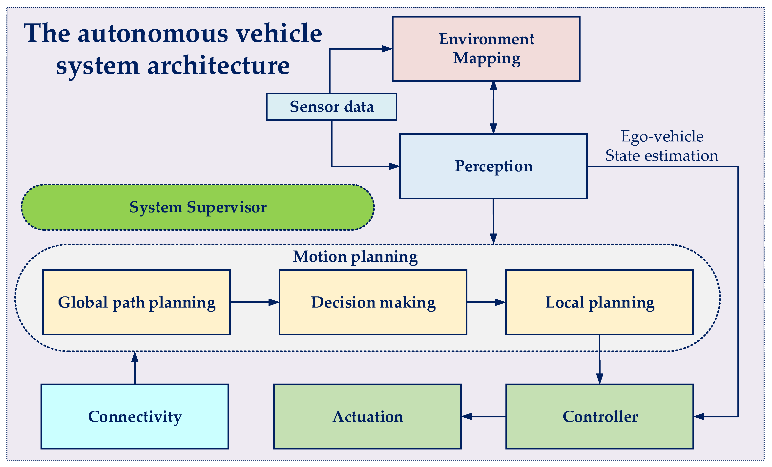
2. Hierarchical Control System

The hierarchical control system consists of global path planning(GPP), decision making, local path planning and control [27] hierarchies from low to high level as shown in Figure 1. The GPP id developed based on HD-map and V2X information by using Dijkstra’s algorithm to select the best route. A series of waypoints from the GPP is first combined with the perception to adjust the behavior of the vehicle. Then, the local path planner employs the behavior to generate an efficient trajectory. Herein, the path is comprised of a set of waypoints with a format < x , y , v > for each waypoint, where x , y are the global coordinate in the Universal Transverse Mercator (UTM) coordinate [11], and v is the speed of the vehicle. Finally, the control commands the car to follow the trajectory by using the longitudinal and lateral controllers. In this section, we neglect the GPP and concentrate on the design of decision making, local path planning, and control.

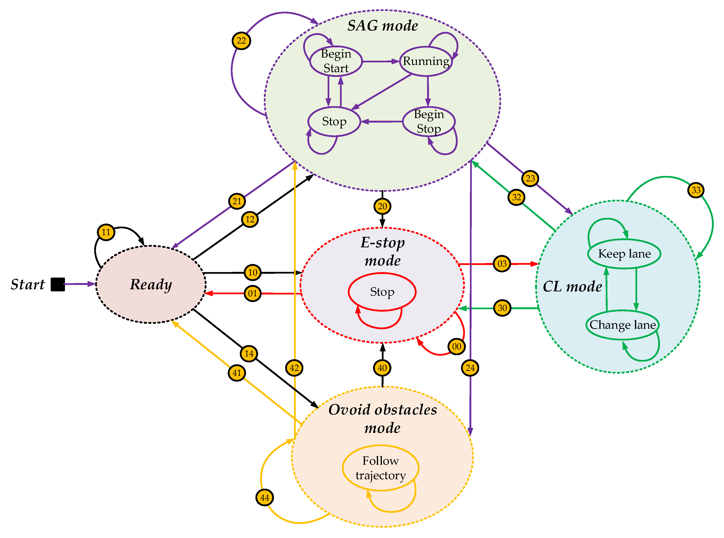
2.1. The Decision-Making Mechanism Based on Two-Stage FSM

The Decision-Making Mechanism (DMM) [28] of SDCs employs FSM to handle the mission planning and behavior on-road driving. The first DMM called the Mission FSM (M-FSM), which manages the vehicle’s missions. The second DMM named the Control FSM (C-FSM) mimics the vehicle’s status on the road. After observing the surrounding object’s trajectory from the perception and the missions data, M-FSM and C-FSM are determined as following in Figure 2. M-FSM is categorized into five classes: Ready, Stop-and-Go (SAG), Change-Lane(CL), E-stop, avoid obstacle mode. In particular, the M-FSM consists of a C-FSM that manages the control states of the vehicle. A human needs to control the vehicle starting or stopping on-road driving by reducing or increasing the acceleration, respectively, to mitigate damage to the engine. Likewise, the SAG mode is designed to mimic all human behaviors mentioned beforehand. When urgent situations appear, the E-stop mode is activated. The CL mode consists of two control states lane-keeping and lane-changing, which actuates when lane changing state is demanded. The obstacle avoiding mode activates when the obstacles have been detected lying on the path. The transition condition is a directed graph in the M-FSM, and the descriptions of all transition conditions in Figure 2 are summarized as following in Table 1.
The data structures, which we infer from Figure 2, are utilized to implement the M-FSM and C-FSM. Each state in FSM requires a resource that is updated over time in the ROS nodes of perception. The use of priority and flag of each state is to prevent access to the same resources. The priority level of the E-stop mode is highest, following by the obstacle avoiding mode, the CL mode, and the SAG mode.

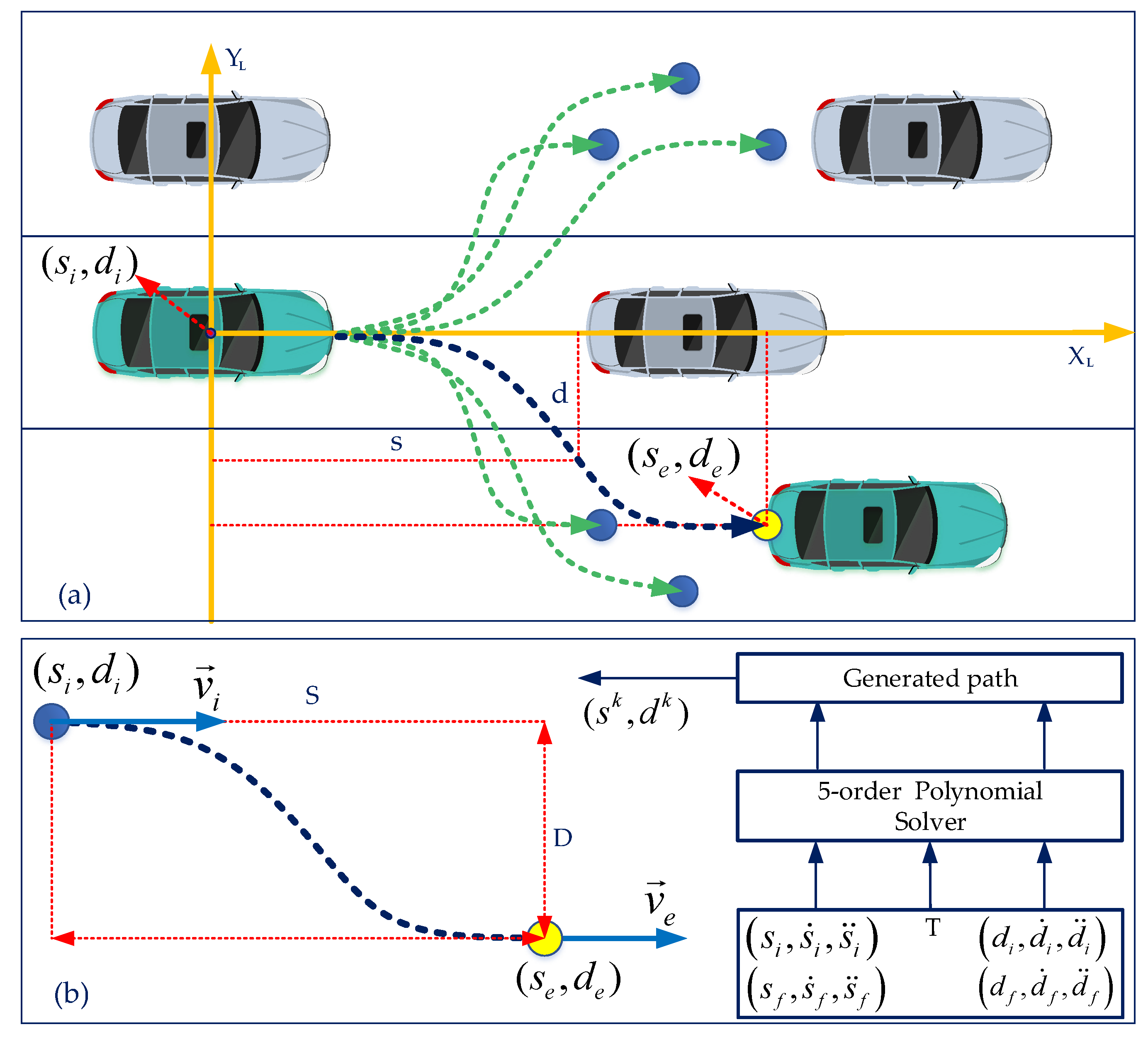
2.2. Local Path Planning

Commonly, the local path planning (LPP) is performed when the mission planning demands and described in Section 2.1. Specifically, LPP needs to find an optimal path to pass the static or dynamic objects while satisfying the kinematic and road shape constraints. The purpose of LPP is to efficiently generate a trajectory for an autonomous robot in the structured or unstructured environment given the temporal start and end position. Moreover, the trajectory, velocity, acceleration, and derivative of the acceleration must smooth during the operation of the vehicle. In this subsection, the jerk minimization based-LPP on the local Frenet coordinate is first presented. Then, an implementation of the hybrid A* algorithm with an occupancy grid map is given.

2.2.1. Optimization-Based LPP on the Local Frenet Coordinate

In this subsection, we perform an optimization-based LPP to generate a route from a start point to a goal. The lane-changing is a typical example and activated whenever motion planning orders. The Frenet coordinate [22,29] applied to represent the vehicle’s planar trajectory into a longitudinal and lateral axis as shown in Figure 3a. The coordinates are represented by s and d parameters, which are the ahead and side distance of the endpoint respect to the initial temporal position respectively. This work employs the temporary Frenet coordinate to efficiently solve an optimization problem, as shown in Figure 3b.
The best way to represent the smooth of a driving route is the derivative of acceleration called jerk. Different from previous work [22,29], an optimization problem for a spatial and temporal path with nonlinear constraints is introduced to minimize the sum of square jerks. The algorithm can also operate in SAG mode as presented in Section 2.1, which is a straightforward problem of this solution.
The problem is solved by minimizing the amount of squared-jerk over the whole temporary trajectory. The results [22,29] indicated that a polynomial function could efficiently represent a trajectory as a function over time. Two quintic polynomial functions are applied to represent a path. Once having the polynomial functions, the trajectory can reconstruct by performing each value corresponding to a discrete-time step. The path regard to s and d coordinate are quintic functions as yielded
z ( t ) = ξ 0 + ξ 1 t + ξ 2 t 2 + ξ 3 t 3 + ξ 4 t 4 + ξ 5 t 5 ,
where t is time (second) started counting from the initial pose of temporary trajectory, and ξ 0 : 5 are the coefficients of the quintic function. The velocity, acceleration and jerk are respectively given by
v z = d z ( t ) d t = ξ 1 + 2 ξ 2 t + 3 ξ 3 t 2 + 4 ξ 4 t 3 + 5 ξ 5 t 4 .
a z = d 2 z ( t ) d t 2 = d v ( t ) d t = 2 ξ 2 + 6 ξ 3 t + 12 ξ 4 t 2 + 20 ξ 5 t 3 .
j z = d 3 z ( t ) d t 3 = d v 2 ( t ) d t 2 = d a ( t ) d t = 6 ξ 3 + 24 ξ 4 t + 60 ξ 5 t 2 .
We assume that the velocity vector of the initial and the end pose have the same length, and their direction coincides with the car heading angle. Therefore, the values at the initial pose { s i , d i } and the endpoint { s e , d e } are selected as
s i = 0 , s ˙ i = v , s ¨ i = 0 d i = 0 , d ˙ i = 0 , d ¨ i = 0 s e = S , s ˙ e = v , s ¨ e = 0 d e = D , d ˙ e = 0 , d ¨ e = 0 .
The cost function of the optimization problem is the sum of the entire square-jerk in the whole temporary trajectory for both s and d direction. The cost is expressed with s and d parameters in term of the quintic function, which is defined by
ξ s , ξ d , T = arg min ξ s , ξ d , T ( t = 0 T j s 2 ( t ) d t + t = 0 T j d 2 ( t ) d t ) = arg min ξ s , ξ d , T t = 0 T 6 ξ 3 s + 24 ξ 4 s t + 60 ξ 5 s t 2 2 d t + t = 0 T 6 ξ 3 d + 24 ξ 4 d t + 60 ξ 5 d t 2 2 d t .
Combining Equations (2) and (3) with their values at initial position (t = 0) and Equation (5). The value of ξ 0 , ξ 1 and ξ 2 for both s and d coefficients are indicated undoubtedly as
ξ 0 = z ( t = 0 ) ξ 1 = v z ( t = 0 ) ξ 2 = 1 2 a z ( t = 0 ) .
Finally, six variables ξ 3 , ξ 4 and ξ 5 for both s and d need to be determined with their constrains at the end pose as yielded by
z T = ξ 0 + ξ 1 T + ξ 2 T 2 + ξ 3 T 3 + ξ 4 T 4 + ξ 5 T 5 v z T = ξ 1 + 2 ξ 2 T + 3 ξ 3 T 2 + 4 ξ 4 T 3 + 5 ξ 5 T 4 a z T = 2 ξ 2 + 6 ξ 3 T + 12 ξ 4 T 2 + 20 ξ 5 T 3 .
Thanks to Equations (6) and (8), the optimization problem is established to solve for T, ξ 3 , ξ 4 and ξ 5 given as
ξ s , ξ d , T = arg min ξ s , ξ d , T J z ( ξ , T ) = arg min ξ s , ξ d , T J s ( ξ 0 : 5 s , T ) + J d ( ξ 0 : 5 d , T ) , s . t . ξ 0 s + ξ 1 s T + ξ 2 s T 2 + ξ 3 s T 3 + ξ 4 s T 4 + ξ 5 s T 5 z s T = 0 ξ 1 s + 2 ξ 2 s T + 3 ξ 3 s T 2 + 4 ξ 4 s T 3 + 5 ξ 5 s T 4 v s T = 0 2 ξ 2 s + 6 ξ 3 s T + 12 ξ 4 s T 2 + 20 ξ 5 s T 3 a s T = 0 ξ 0 d + ξ 1 d T + ξ 2 d T 2 + ξ 3 d T 3 + ξ 4 d T 4 + ξ 5 d T 5 z d T = 0 ξ 1 d + 2 ξ 2 d T + 3 ξ 3 d T 2 + 4 ξ 4 d T 3 + 5 ξ 5 d T 4 v d T = 0 2 ξ 2 d + 6 ξ 3 d T + 12 ξ 4 d T 2 + 20 ξ 5 d T 3 a d T = 0 T > 0 .
The results of optimization problem in Equation (9) are obtained in Figure 4. It should be noticed that using constrain T > 0 in the experiment approximately increases twice the computational cost. Therefore, we drop constrain T > 0 to relax the optimization problem, later only need to check the condition. For different velocities, the optimal trajectory is solved and presented as the solid blue line in Figure 4. As observed from Figure 4, when v large, it significantly affect the results. In this case, if the value of T is selected slightly different from the optimal value, the result can not produce an optimal trajectory. Moreover, when the travel time T from the initial point to end point is known, we can easily find ξ 3 , ξ 4 and ξ 5 by using Equations (7) and (8) as follows
T 3 T 4 T 5 3 T 2 4 T 3 5 T 4 6 T 12 T 2 20 T 3 ξ 3 ξ 4 ξ 5 = z t = T ( ξ 0 + ξ 1 T + ξ 2 T 2 ) v z t = T ( ξ 1 + 2 ξ 2 T ) a z t = T 2 ξ 2 .
The last step is developing the quintic function of the s and d axis to reconstruct the trajectory at each discrete time as shown in Figure 3b. The obtained results are presented in Figure 5. To reduce the computational complexity, a practical solution uses a lookup table determined by the offline optimization solving process. Whenever the DMM informs lane changing, the lookup table is utilized online to find the optimal time of T, then solve the linear in Equation (10) to get the optimal path.

2.2.2. Obstacle Avoidance Based on Hybrid A* Algorithm

One of the important features of the path-planning module in an autonomous vehicle framework is the obstacle avoidance mechanism [16,30]. This mechanism is desired when an autonomous vehicle must detour the predefined global path in order to avoid any hindrance. Typical examples of such environments are of car crash-like obstacles, or construction sites on the highways. The path planner, upon receiving the information from the perception module about an obstruction in the way, activates the obstacle avoidance mechanism. Based on the information from the perception module and global path, sub-goals of starting and goal poses of the vehicle are defined, and an ideal path is generated that takes non-holonomic constraints into account. The realtime hybrid A*-based LPP is performed that mainly inherits the implementation of [31,32]. The algorithm is performed when DMM requests by providing start and goal location and occupancy grid map as the inputs. The goal is selected from the global path planning, whereas the perception within a sliding window continuously updates the local grid map. The algorithm starts with the initialization by generating a collision lookup table and obstacle distance lookup table. The Reed Shepp curves are calculated for the constrained heuristics, whereas an A* search was conducted for the unconstrained heuristics. The analytical collision-free path is fed to the smoother that optimizes the obstacle distances and treats it for smoothness. Later, the refined path is fed forward to the control module. The main improvement compared with the previous research [31] is a large static occupancy grid map is stored as initialization and updated during the operating of this algorithm. The local region about the obstacle is employed for path planning. This methodology enables the safe path generation when dealing with the uncertainty of dynamic objects from the perception.

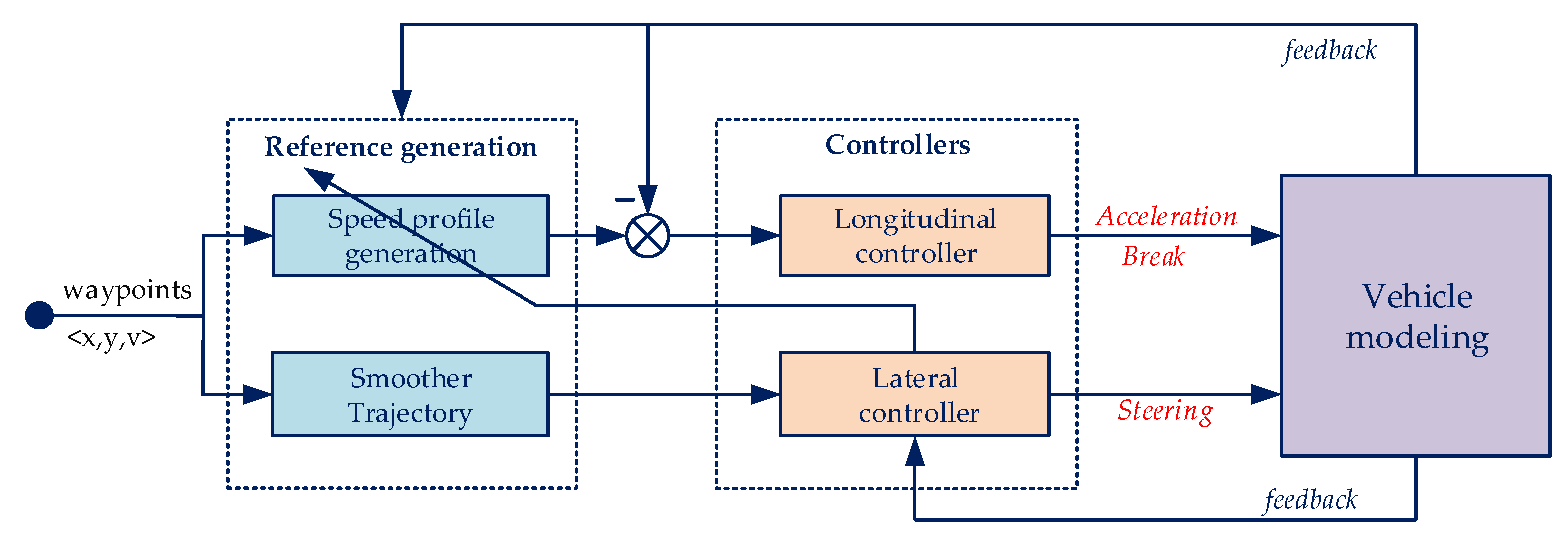
2.3. Vehicle Control Strategy

The local path planning generates a local trajectory plus target speed. Then, the vehicle is commanded to follow the local path towards reference velocities. The control architecture includes longitudinal and lateral control [33]. The longitudinal controller asks the vehicle to follow the desired speed by acting acceleration, whereas the lateral controller manipulates the lane tracking by adjusting the steering turn. The controller architecture is demonstrated as in Figure 6. The curve-level of trajectory is used to create the speed profile generation (SPP). The target speed of DMM feeds directly into the longitude controller if it is greater than the speed after the SPP. In contrast, DMM speed is utilized.

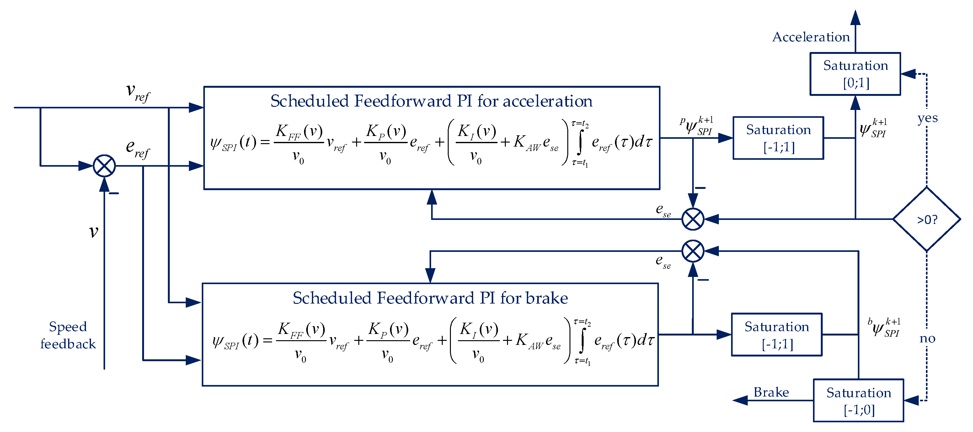
2.3.1. The Longitudinal Controller

The characteristics of the model are required to design a controller efficiently. However, the full modeling of a vehicle entails complexity and nonlinearity [34]. Besides, it is hard or impossible to identify the parameters of vehicle modeling by describing physical relationships. Instead, we identify the model by using a simple method where the workstation command as the input and the longitudinal velocity as the output. The model is represented as a second-order function with a time delay [34], as yielded in Equation (11).
G P v ( s ) = V ( s ) A c c ( s ) = K P 1 s + K P 1 T P 2 s 2 + T P 1 s 2 + T P 0 e s τ d .
Although the parameters of the model (11) depend on velocity and road terrain, the model’s characteristics are helpful to adjust the controller parameters. Researchers [16,17,20,25,30,34] did not present how to tune the controller into practice. In this work, we first collect data, then identify the vehicle model, next analyze its properties, and finally design the controllers. The SFF-PI controller [35] as in Figure 7 tracks the feedback signal including velocity error, windup affecting before and after saturation, and the vehicle velocity yielded as
ψ S P I ( t ) = K F F ( v ) v 0 v r e f + K P ( v ) v 0 e r e f + K I ( v ) v 0 + K A W e s e τ = t 1 τ = t 2 e r e f ( τ ) d τ ,
where e r e f is the difference between the desired and measured velocity, e s e is the error of output before and after the saturation block which limits the acceleration and brake within −1 and 1. K F F ( v ) , K P ( v ) , K I ( v ) are respectively feedforward, propagation, integration coefficient, which depend on the velocity, and v 0 is the nominal velocity of vehicle.
To implement the controller, we need to transform Equation (12) from continuous-time to discrete-time domain with a period of T. So, the output of the controller at time t = k T is given as
ψ S P I k = K F F v 0 v r e f k + K P ( v k ) v 0 e r e f k + K I ( v k ) v 0 + K A W e s e k T i = 0 k e r e f k .
Similarly, the output at the next time step t = ( k + 1 ) T is
ψ S P I k + 1 = K F F v 0 v r e f k + 1 + K P ( v k + 1 ) v 0 e r e f k + 1 + K I ( v k + 1 ) v 0 + K A W e s e k + 1 T i = 0 k + 1 e r e f k + 1 .
The integration can be obtained by using the recursion
Γ k + 1 = i = 0 k + 1 e r e f k + 1 = e r e f k + 1 + i = 0 k e r e f k = e r e f k + 1 + Γ k .
The proposed architecture of the longitudinal controller is illustrated in Figure 7. Using the recursive form of Equations (14) and (15) to implement the SFF-PI controller which is shown in Algorithm 1. Herein, the control algorithm is processed at each interrupt event of a timer. Line 2 gets the desired and measured velocities. Then line 3 calculates the error velocity. In line 5, the scheduled PI parameters are searched in a lookup table saved in the program. The integration value can be achieved by utilizing Equation (15) as in line 6, and the output value is processed using Equation (14) in line 7. From line 8 to line 10, if the control values before and after saturation are different, it needs to re-handle Equation (14) to get new e s e k + 1 . The controller must apply accelerating or braking to obtain the best control performance. To perform that, we only need to apply acceleration if it is more than zero, otherwise braking is used as from line 14 to line 19.
In summary, The longitudinal controller based on the SFF-PI is designed as follows
Step 1—recording data: the acceleration range [0, 1] is executed and recorded as the input, also the output is the observed velocity. Similarly, when the vehicle operates at a nominal speed, the braking force range [−1, 0] is employed.
Step 2—identifying: accelerating and braking model are identified by using the second-order modeling with a time delay.
Step 3—designing: the SFF-PI controller is designed and tuned to obtain the best result.
Step 4—evaluating: Algorithm 1 is run with the parameters tuned in Step 3. In practice, the parameters should be slightly adjusted.
Algorithm 1: Longitudinal control algorithm based on SFF-PI.
Applsci 10 03543 i001

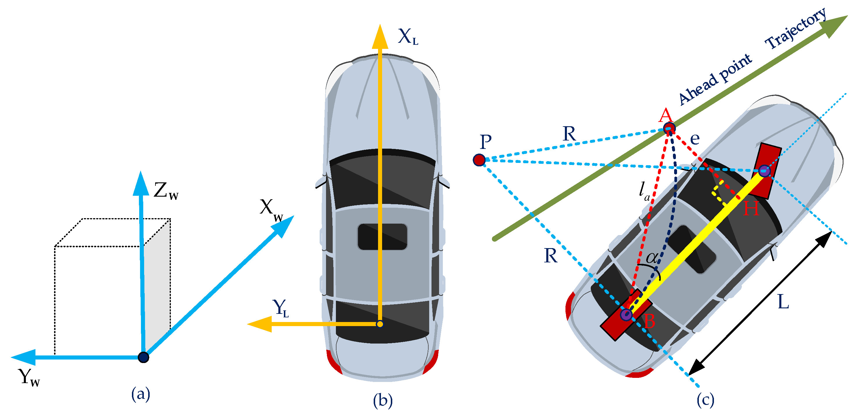
2.3.2. Adaptive-Pure Pursuit Algorithm Based-Lateral Controller

To pursue a trajectory that is provided by LPP, the lateral controller is needed. Recently, the state-of-the-art lateral controller is Model Predictive Control (MPC) [16,20,36], which can effectively address the problem with high accuracy. However, this method is complex, and it requires high computational cost and resources. Besides, the processing time of MPC controller is approximately 10 ms in practice, so it can cause a delayed signal. Although the optimal controllers such as feedforward-LQR can achieve high accuracy, its robustness is not guaranteed due to the disturbances [37]. Geometry based-path tracking is one of the most common methods of path tracking algorithms in robotics. This solution finds the relationship between the vehicle and the path by the geometric constraints. One of the most famous geometry-based controllers is Stanley, which was introduced and implemented in Stanley robot in DARPA Grand Challenge in 2005 [16,30]. This approach uses the front-wheel position as a nonlinear feedback function of the cross-track error. The controller operates smoothly in the highway driving, but it is fair to deal with disturbances. Furthermore, the Stanley method encounters a discontinuity path tracking problem while the Pure Pursuit Controller (PPC) is more robust. Although the PPC is not precise as the state-of-the-art methods in high-speed scenarios, the PPC is selected due to its stabilization to disturbances [16]. In this paper, we present the implementation of an adaptive-PPC for path tracking with an explicit algorithm. The path curvature is described in Figure 8c given as
χ = 1 R = 2 sin ( α ) l a ,
where l a is the look-ahead distance determined from the rear axle pose to the desired path, R is the radius of the circle passing through points A and B with having a tangent at point A, α is the angle between the vehicle heading and the look-ahead direction. The steering angle is calculated by using the bicycle model and Equation (16) as follows
ψ p p = tan 1 ( χ L ) = tan 1 ( 2 L sin ( α ) l a ) .
Using the relationship of cross-track error e in Figure 8c, Equation (16) can be written as
sin ( α ) = e l a χ = 2 e l a 2 .
The look-ahead l a is linearly proportional to the longitudinal velocity of the vehicle v r . Thus l a = κ v r . Finally, using Equations (17) and (18), we haves
ψ p p = tan 1 2 L sin ( α ) κ v = tan 1 2 e L l a 2 .
where l a is set to the minimum and maximum values of 3 m and 22 m, respectively. As reported in [37], the value of κ effects the stability of the system. Roughly speaking, increasing or decreasing the value of κ is the trade-off between smoothness and precision tracking. However, the value of κ is unreliable if it is excessively small or large which causes instability or poor tracking. The value of κ is tuned and implemented as in [38]. Therefore, the looking ahead distances are adapted as follows
l a = 3 ; v < 15 k p h 0.76 v 8.4 ; 15 k p h v 40 k p h 22 ; v > 40 k p h .
The vehicle speed directly affects the stabilization such as the slipping and rolling. So, the target speed needs to limit depending on the road curvature [38] as yields
v g ( ρ + ϑ ) χ = g ( ρ + ϑ ) l a 2 2 e ,
where g is gravity, ρ is the road super-elevation smaller than 6% in the urban environment, and ϑ is the side friction factor bounded to 0.1 for dry road [38]. Therefore, we bound the target speed as
v 0.9 l a e
Finally, we implement the lateral controller described in Algorithm 2 with a timer interruption of 10 ms. Herein, the look-ahead distance is first calculated, then the local path is converted to the vehicle coordinate. Next, the closest waypoint and ahead waypoint are found by using Algorithms 3 and 4, respectively. The final step is calculating the limited speed and steering angle. Note that e is y-coordinate of the ahead-waypoint in the local frame.
Algorithm 2: The lateral controller and velocity planning algorithm based on PPC.
Applsci 10 03543 i002
Algorithm 3: Find the closest waypoint to the ego-vehicle.
Applsci 10 03543 i003
Algorithm 4: Find the ahead waypoint in the reference trajectory.
Applsci 10 03543 i004

3. Experimental Results

After developing the hierarchical control system in Section 2, this section provides experimental results of the decision making, local path planning and control. Firstly, the vehicle platform, hardware, and software are presented. Secondly, we demonstrate the robustness of the control system. Finally, the local path planner is given with the performance in both structured and unstructured environments.

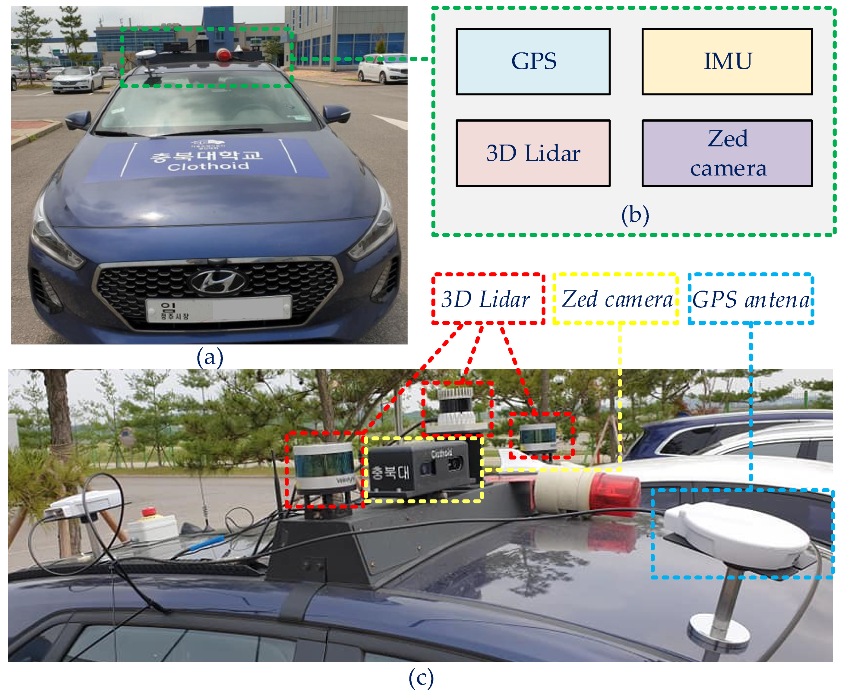
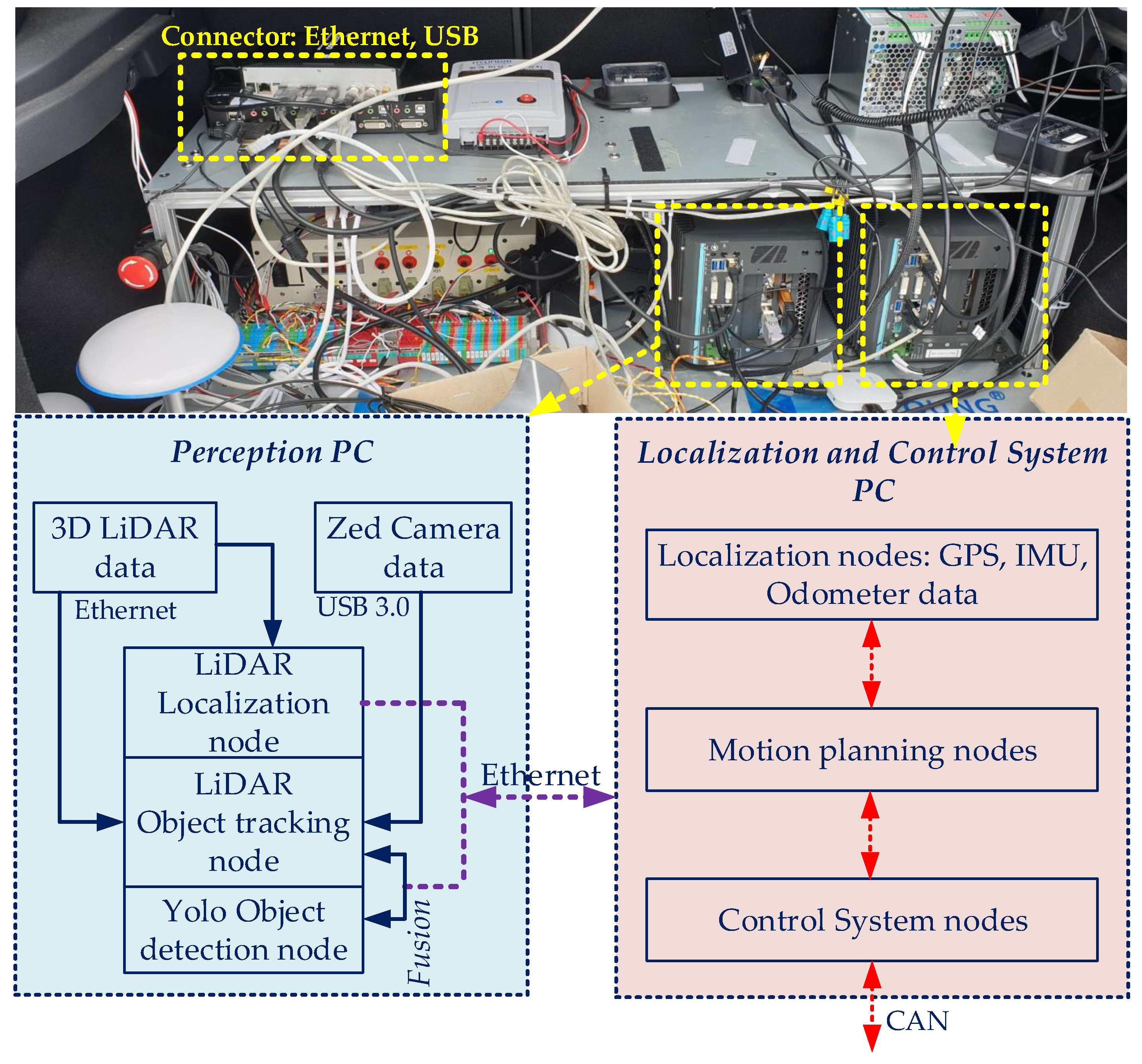
3.1. The System Integration of Autonomous Vehicle

The self-driving car uses the model Hyundai I-30 platform with the configuration illustrated as in Figure 9.
The autonomous vehicle is equipped with various sensors to enhance the perception. The sensors system consists of 3D Light Detection and Ranging (3D LiDAR), Zed-camera, GPS, IMU, and encoders. The computational devices use two computers with the configurations as Xeon X5690 processors, NVIDIA GeForce GTX-1080Ti, 32 GB RAM, 512 GB SSD, and networking gear as shown in Figure 10.
The perception workstation (PW) handles Object Detection and Tracking (ODAT) by fusing 3D LiDARs and cameras. The Control System Workstation (CSW) performs the localization by using GPS, IMU and encoders [39] and the controller. The perception, localization, and control tasks employ the Robot Operating System (ROS) middle-ware version-Kinetic Kame [15] on top of Ubuntu 16.04.5 LTS. The development utilizes two workstations connected by the ROS TCP/IP protocol. In Figure 10, the PW runs a deep learning node using YOLO v3 [40] and 3D LiDARs for ODAT with IMM-UKF-JPDAF algorithm [19]. The CSW handles the localization by applying the sensor fusion technique of GPS and IMU [39]. The control system includes global path planning based on an HD map node, local path planning node, and controller node. We notice that LiDAR object detection and LiDAR localization must work in one computer because of latency transportation of LiDAR data through the Ethernet.

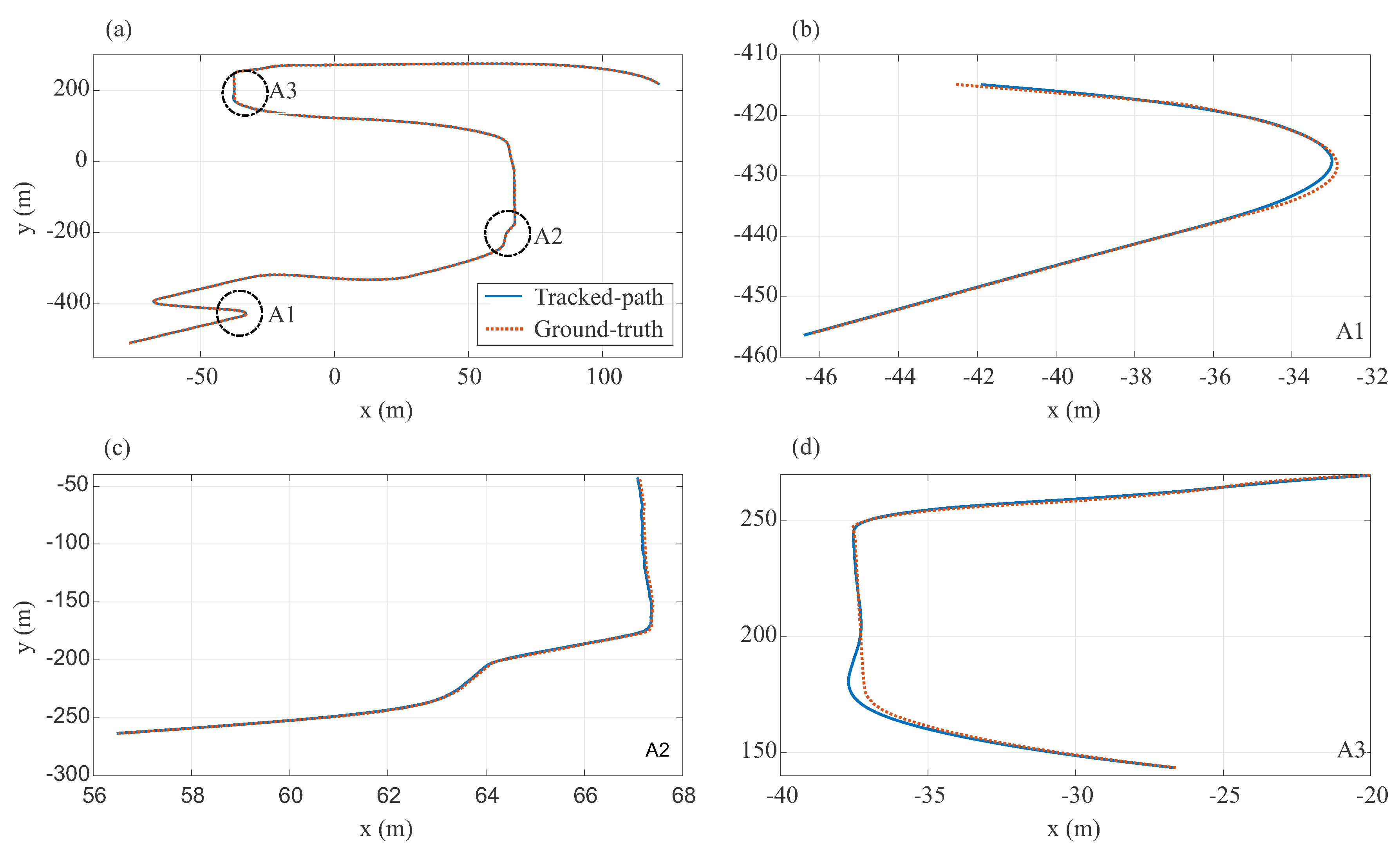
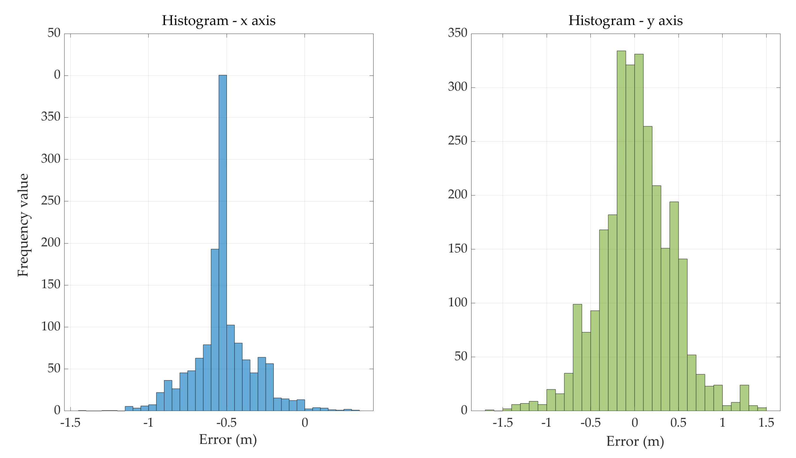
3.2. The Robustness of the Path Tracking Controller

Firstly, we implement path-tracking algorithm based on adaptive-PPC in Section 2.3.2. Then, the working performances in a proving ground are analyzed. The results show that the algorithm works efficiently and performs missions successfully in the test. The tracking results are visualized in Rviz as shown in Figure 11. The outcomes indicate that the lateral controller obtains the stabilization and robustness to disturbances such as terrain, rolling resistance, and aerodynamic effect. In the common areas with small curvature such as regions 1, 2, 3, and 4 handle well with the low slip respect to the reference trajectory. Although Region 6 and 7 have convex curvatures, the lateral controller also performs well.
Figure 12 presents the path tracking results in structured environments. The data is recorded with a bag file, then processing in MATLAB-Robotics System Toolbox. Figure 12b–d are cropped from Figure 1 working at high-curvatures. The path tracking algorithm operates well with small tracking errors in this trial. The hardest task is shown in zone 5 with a concave curve, and the vehicle performs comfortably while the vehicle speed is around 12 kph. It should be remarked that, the adaptive-PPC effortlessly tracks the center of the road while the human is troublesome to conduct this challenge. Roughly speaking, the adaptive-PPC can outperform humans in this test.To check the performance of adaptive-PPC, we define the root square error of the path tracking algorithm as follows
ς x = i = 1 N δ x 2 N = i = 1 N ( P x P x r e f ) 2 N ; ς y = i = 1 N δ y 2 N = i = 1 N ( P y P y r e f ) 2 N ; ς = ς x + ς y 2 ,
where ς x and ς y are the Root Mean Square Error (RMSE) of the path tracking in x and y-axis, and ς represents the average error in both x and y-axis. Furthermore, δ x and δ y denote the error of measured and ground-truth point at each time step. P x and P x r e f are x coordinate of each position and reference point at each measured time step, respectively. P y and P y r e f are similar for y coordinate. The results of path tracking error in the structured environment in Figure 12 shown in Table 2.
The overall error of the tracking algorithm is around 6 mm per waypoint. The errors at high-curvature approximately are 10 to 25 mm per waypoints. We also demonstrate the error in terms of the histogram as shown in Figure 13.

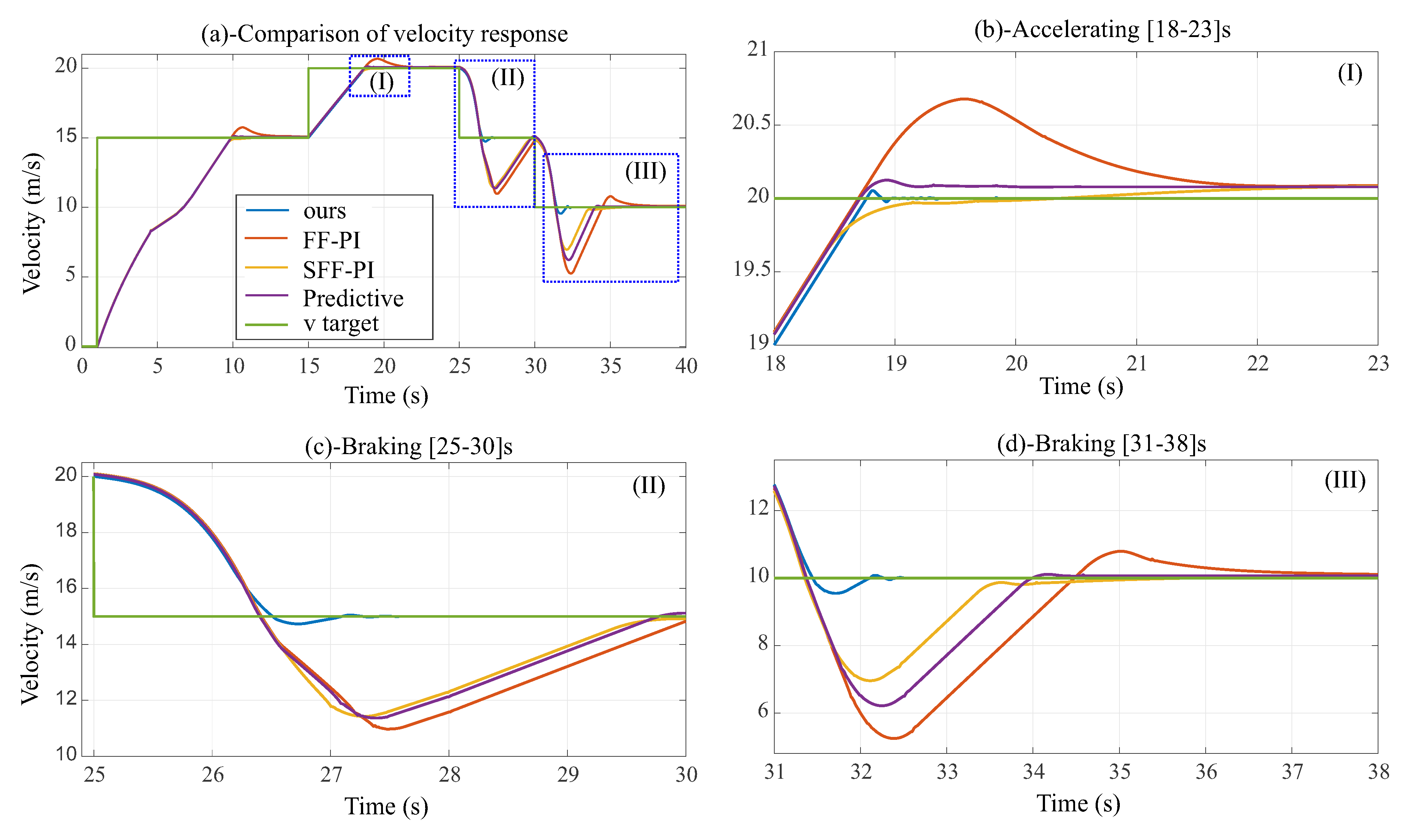
3.3. Velocity Tracking Based on SFF-PI Controller

The vehicle modeling uses MATLAB and Simulink with the dynamic model specified in Vehicle Dynamics Blockset. In this simulation, the vehicle model with one degree-of-freedom (1DOF) was used. A simulation model was developed to compare control strategies between a feedforward PID [26], a SFF-PI [26], a Predictive [35] controller and ours approach as shown in Figure 14. Our method uses two SFF-PI controllers described in Algorithm 1, and the controllers have also tuned the parameters. We implement the SFF-PI controller as in Algorithm 1. The parameters for the accelerating controller are updated as follows
K F F = 0.1 ; K A W = 1 ; v 0 = 5 ; { K P , K I } = { 0.2 , 100 } ; v < 5 { 6 v 29 , 100 v } ; 5 v < 10 { 6 v 30 , 100 v } ; 10 v < 20 { 100 , 2100 } ; v 20 .
We also adjust the parameters of the braking controller as
K F F = 0.2 ; K A W = 1 ; v 0 = 5 ; { K P , K I } = { 0.005 , 100 } ; v < 5 { 0.09 v 0.35 , 10 v + 100 } ; 5 v < 10 { 0.1 v 0.4 , 10 v + 100 } ; 10 v < 15 { 0.1 v 0.5 , 20 v + 100 } ; 15 v < 20 { 1.2 , 250 } ; v 20 .
The results in Figure 14 indicate that our controller outperforms other controllers. Figure 14b shows the accelerating process of ours has the best outcome. The most outstanding result was working on the braking process, as in Figure 14c,d.
In a real test, the performance of our longitudinal controller is provided in Figure 15. The output speed tracks the desired velocity with a small steady-state error. The result in Figure 15 is a part of the complete result in the proving ground. The desired velocity is generated by using curvature information indicated in Section 2.3.2. The response velocity tracks with a small steady-state error without overshoot because of the limit of acceleration and brake in [−0.8;0.8]. The setting time from 9 kph to 40 kph is approximately 5.5 s. However, if we do not bound the throttle, it can achieve around 4 s as the simulate result in Figure 14. In the braking situation, the design speed can archive from 40 kph to 15 kph for about 5 s.

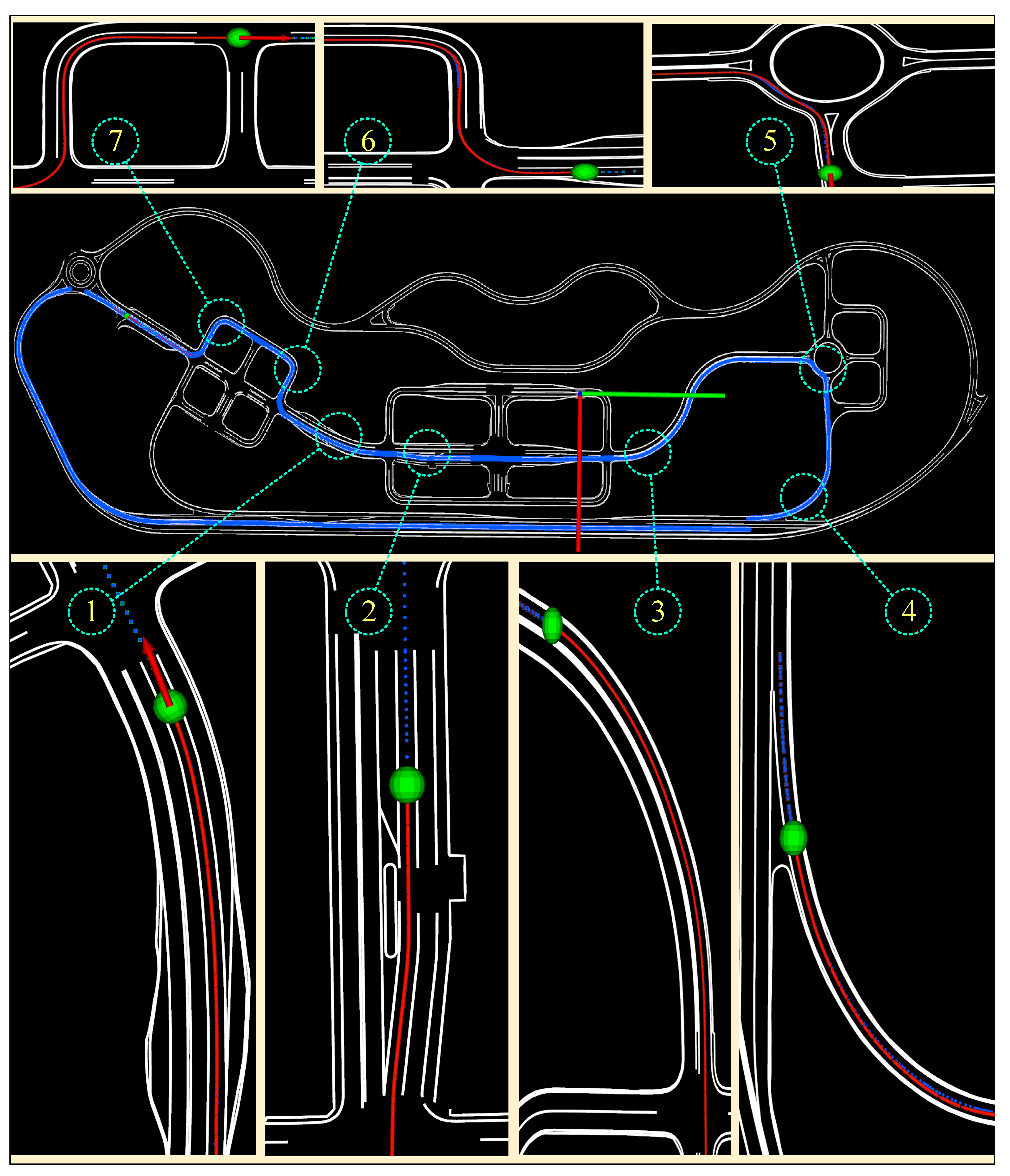
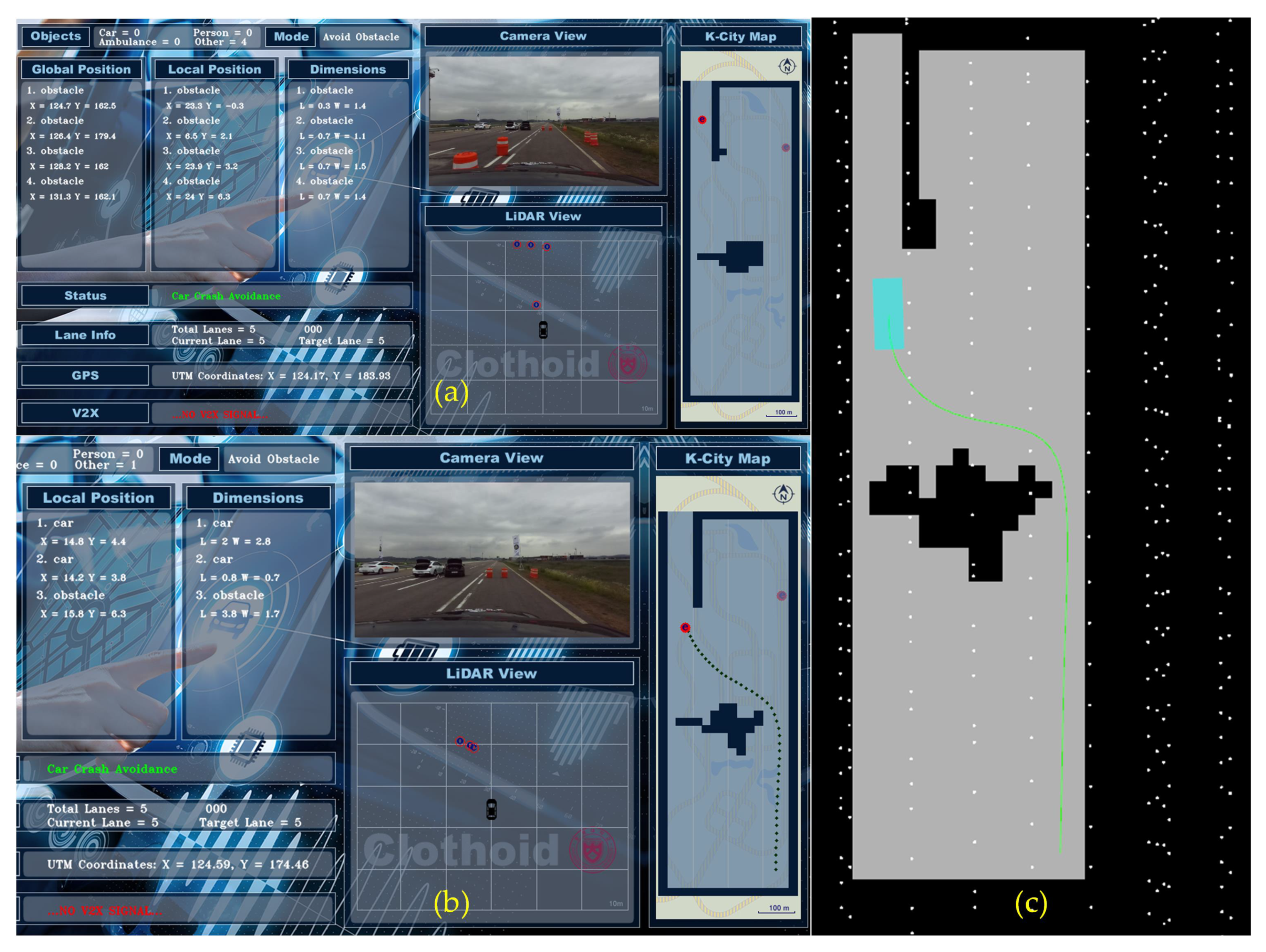
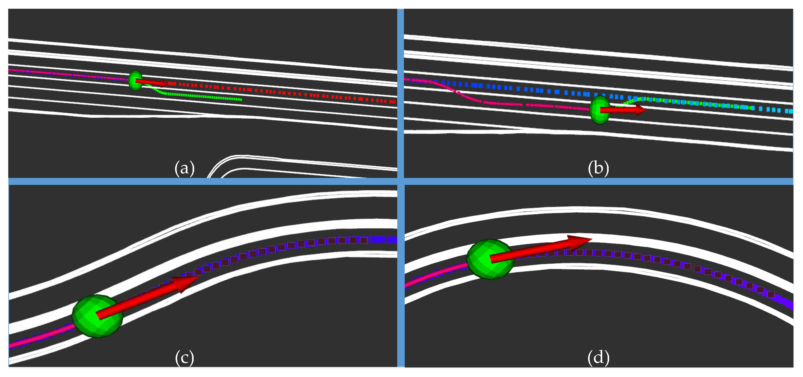
3.4. The Local Path Planning

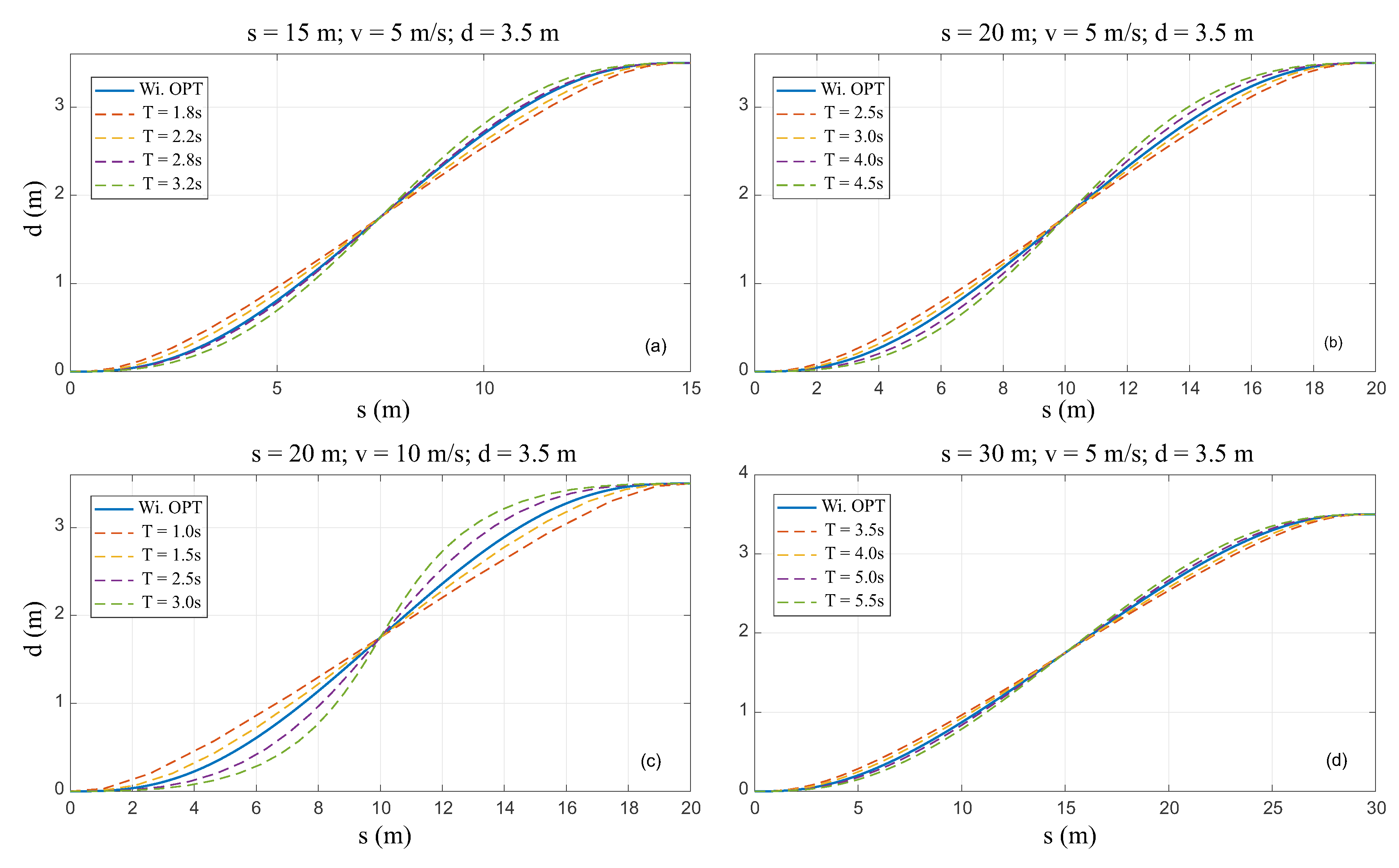
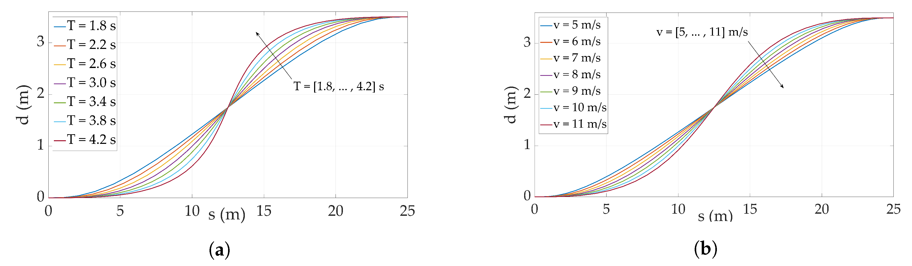
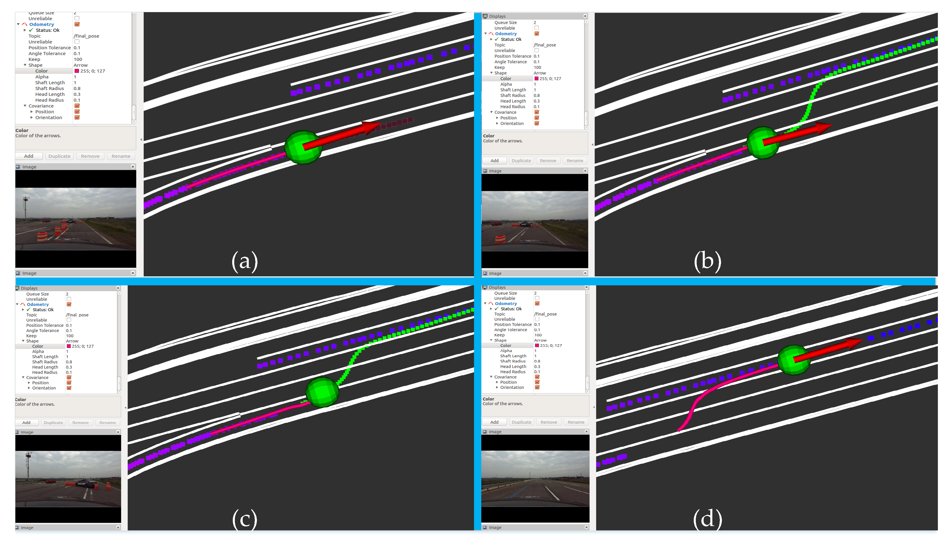
3.4.1. The Local Path Generation

The results of local path planning are presented in Figure 16. The lane-changing task is performed to produce a smooth route with the minimum jerk reported in Section 2.2.1. The lane-changing to the right lane as shown in Figure 16a, after that if the left lane safe, the vehicle change back to the left lane as visualized in Figure 16b. In Figure 16c,d, the result shows a new trajectory by using the three-order polynomial function in the Appendix A.2. The main drawback of this method is that it can not work well in high curvature as in Figure 11 regions 5–7.

3.4.2. The Local Path with Hybrid A*

Figure 17 shows two instances of custom-built visualizer. The first instance is when the perception module notices obstacles in the global path and initiates the path planning module. Thus the occupancy grid map starts to populate. The second instance is of a detoured path that is being followed by the vehicle. The result of the local path with hybrid A* in real-world experiments are demonstrated in Rviz in Figure 18. In Figure 18a, when the vehicle enters the obstacle zone where the perception detects. The vehicle follows a straight path until finding a route to pass the obstacles as shown in the Figure 18b. The green path is continuously updated and published to the control until the car reaches the goal point Figure 18c,d.

4. Conclusions

In this paper, we address the analysis and design of a hierarchical control system for a self-driving car in the urban environment. Besides, this work also presents the tuning and implementation of the system into practice. The progress addresses the hierarchical control system from the low to high-level control. A raw-trajectory is generated from the global path planning with the aid of an HD map and wireless communication V2X. Firstly, the decision-making mechanism is proposed to handle the missions and control states on the way by implementing the two-stage FSM. Then, the local path planning selects a decision and utilizes it to produce a reference trajectory to the control. Secondly, the local path planning generates an online trajectory with the jerk minimization and the hybrid A* to secure lane-change and avoid obstacles, respectively. The controllers operate the vehicle by commanding throttle, brake, steering angle to follow the local route efficiently with longitudinal and lateral controllers. We implement this work successfully with ROS middleware. The on-going works are the implementation of the autonomous vehicle working robustly and efficiently under all-weather and terrain conditions of the urban environment.

Author Contributions

Methodology, N.D.V., M.S., D.K. and G.-W.K.; N.D.V., M.S. and D.K. conducted the experiments and analyzed the results; N.D.V. wrote the original draft; G.-W.K. reviewed and edited the draft. Supervision, G.-W.K. All authors have read and agreed to the published version of the manuscript.

Funding

This research was supported in part by the National Research Foundation of Korea(NRF) grant funded by the Korea government(MSIT) (No. 2018006154) and in part by the MSIT(Ministry of Science, ICT), Korea, under the ITRC(Information Technology Research Center) support program(IITP-2020-2016-0 00465) supervised by the IITP(Institute for Information & communications Technology Planning & Evaluation).

Conflicts of Interest

The authors declare no conflict of interest.

Appendix A.

Appendix A.1. Coordinate Transformation

To implement local path planning and control algorithms, we need to transform between local (vehicle) and global frame (UTM coordinate), as shown in Figure 8. The transformation of a local point in vehicle frame { c } to world frame { W } using the homogeneous transform is yielded in Equation (A1).
W x w W y w 1 = W R C W p C 0 1 C x w C y w 1 = T C x w C y w 1 ( T S E ( 3 ) ) ,
where y a x represents the transformation from x frame to y frame, R is rotation matrix. Equation (A1) can be written as
W x w = C x w cos ( W θ C ) C y w s i n ( W θ C ) + W x C W y w = C y w s i n ( W θ C ) + C y w c o s ( W θ C ) + W y C .
A global point in world frame transforms to local coordinate as shown in Equation (A3)
C x w C y w 1 = T 1 W x w W y w 1 = W R C W p C 0 1 1 W x w W y w 1 = W R C 1 W R C 1 W p C 0 1 W x w W y w 1 .
Equation (A3) can be written as
Δ x = W x w W x C Δ y = W y w W y C C x w = Δ x cos ( W θ C ) + Δ y s i n ( W θ C ) C y w = Δ y cos ( W θ C ) Δ x s i n ( W θ C ) .

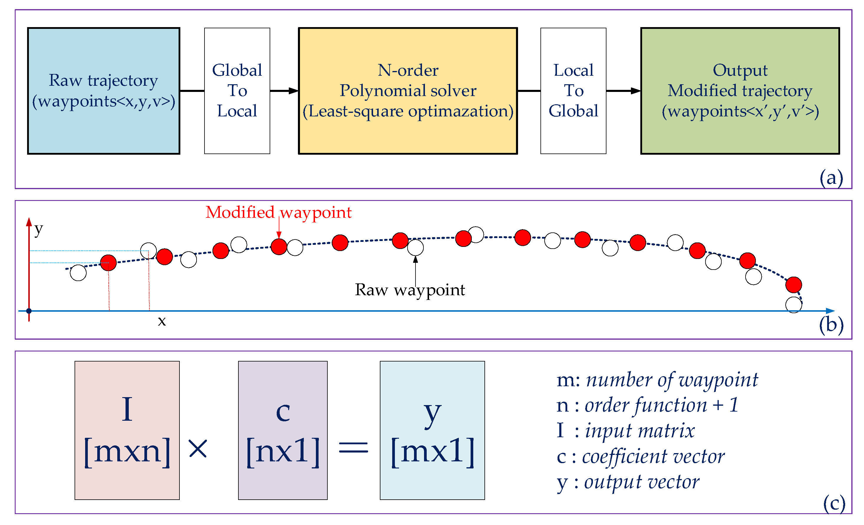
Appendix A.2. Smoother Trajectory

The smoother trajectory algorithm performs the 3-order polynomial by solving a least-square problem with QR decomposition. The polynomial function can also estimate the curve level by comparing the error of heading angle and tangent at the closest point to the vehicle.
The problem is to find parameter c with I c = y as shown in Figure A1. It can convert to a least square problem c = arg min c I c y 2 . This problem has several techniques to solve such as QR, SVD, Cholesky factorization with the computational cost 2 m n 2 2 n 3 3 , 14 m n 2 + 8 n 3 , and n 2 ( 2 m + n 3 ) flops, respectively. In general, QR factorization is selected due to lowest complex, so I = Q m x n R n x n . The use of QR is shown as
I T I = ( Q R ) T Q R = R T R R T R c = I T y = R T Q T y R c = Q T y .
We use C++ Eigen-library to serve QR factorization.
Figure A1. Smoother trajectory using n-order polynomial function based on least square optimization. (a) The overview of the smoother path algorithm, <x,y> is the coordinate of a point in the global frame, v is the velocity of the vehicle. (b) the waypoints before and after operating the smoother algorithm. (c) The dimension of matrices in the least square problem.
Applsci 10 03543 g0a1

References

  1. Singh, S. Critical Reasons for Crashes Investigated in the National Motor Vehicle Crash Causation Survey. March 2018. Available online: https://crashstats.nhtsa.dot.gov/Api/Public/ViewPublication/812506 (accessed on 10 March 2020).
  2. SAE International. Taxonomy and Definitions for Terms Related to Driving Automation Systems for On-Road Motor Vehicles; SAE International: Warrendale, PA, USA, 2019. [Google Scholar]
  3. Hawkins, A.J. Waymo is first to put fully self-driving cars on US roads without a safety driver. The Verge, 27 August 2019. [Google Scholar]
  4. Available online: https://en.wikipedia.org/wiki/DARPA_Grand_Challenge (accessed on 10 March 2020).
  5. Buehler, M.; Iagnemma, K.; Singh, S. The 2005 DARPA Grand Challenge: The Great Robot race; Springer: New York, NY, USA, 2007; Volume 36. [Google Scholar] [CrossRef]
  6. ELROB, The European Land Robot Trial (ELROB). Available online: http://www.elrob.org/ (accessed on 10 March 2020).
  7. Xin, J.; Wang, C.; Zhang, Z.; Zheng, N. China Future Challenge: Beyond the Intelligent Vehicle. IEEE Intell. Transp. Syst. Soc. Newslett. 2014, 16, 8–10. [Google Scholar]
  8. Available online: http://www.hyundai-ngv.com/en/tech_coop/sub05.do (accessed on 10 March 2020).
  9. Available online: https://selfdrivingcarx.com/google-waymo/ (accessed on 10 March 2020).
  10. Tesla Motors: Model S Press Kit. Available online: https://www.tesla.com/presskit/autopilot (accessed on 10 March 2020).
  11. Kato, S.; Takeuchi, E.; Ishiguro, Y.; Ninomiya, Y.; Takeda, K.; Hamada, T. An open approach to autonomous vehicles. IEEE Micro 2015, 35, 60–68. [Google Scholar] [CrossRef]
  12. Fan, H.; Zhu, F.; Liu, C.; Zhang, L.; Zhuang, L.; Li, D.; Zhu, W.; Hu, J.; Li, L.; Kong, Q. Baidu Apollo em motion planner. arXiv 2018, arXiv:1807.08048. [Google Scholar]
  13. NVIDIA. Driveworks SDK. Available online: https://developer.nvidia.com/driveworks (accessed on 10 March 2020).
  14. CommaAI. OpenPilot. Available online: https://github.com/commaai/openpilot (accessed on 10 March 2020).
  15. Available online: http://wiki.ros.org/kinetic/ (accessed on 10 March 2020).
  16. Paden, B.; Čáp, M.; Yong, S.Z.; Yershov, D.; Frazzoli, E. A Survey of Motion Planning and Control Techniques for Self-Driving Urban Vehicles. IEEE Trans. Intell. Veh. 2016, 1, 33–55. [Google Scholar] [CrossRef] [Green Version]
  17. Badue, C.; Guidolini, R.; Carneiro, R.V.; Azevedo, P.; Cardoso, V.B.; Forechi, A.; Jesus, L.; Berriel, R.; Paixão, T.; Mutz, F.; et al. Self-Driving Cars: A Survey. arXiv 2019, arXiv:1901.04407. [Google Scholar]
  18. Zhang, J.; Singh, S. LOAM: Lidar Odometry and Mapping in Real-time. Robot. Sci. Syst. 2014, 2. [Google Scholar] [CrossRef]
  19. Sualeh, M.; Kim, G.-W. Dynamic Multi-LiDAR Based Multiple Object Detection and Tracking. Sensors 2019, 19, 1474. [Google Scholar] [CrossRef] [Green Version]
  20. Pendleton, S.D.; Andersen, H.; Du, X.; Shen, X.; Meghjani, M.; Eng, Y.H.; Rus, D.; Ang, M.H. Perception, Planning, Control, and Coordination for Autonomous Vehicles. Machines 2017, 5, 6. [Google Scholar] [CrossRef]
  21. Gu, T.; Atwood, J.; Dong, C.; Dolan, J.M.; Lee, J.W. Tunable and stable real-time trajectory planning for urban autonomous driving. In Proceedings of the 2015 IEEE/RSJ International Conference on Intelligent Robots and Systems (IROS), Hamburg, Germany, 28 September–3 October 2015; pp. 250–256. [Google Scholar]
  22. Werling, M.; Ziegler, J.; Kammel, S.; Thrun, S. Optimal trajectory generation for dynamic street scenarios in a Frenét Frame. In Proceedings of the IEEE International Conference on Robotics and Automation, Anchorage, AK, USA, 3–7 May 2010; pp. 987–993. [Google Scholar]
  23. Bojarski, M.; Del Testa, D.; Dworakowski, D.; Firner, B.; Flepp, B.; Goyal, P.; Goyal, P.; Jackel, L.D.; Monfort, M.; Muller, U.; et al. End to end learning for self-driving cars. arXiv 2016, arXiv:1604.07316. [Google Scholar]
  24. Van Dinh, N.; Kim, G. Fuzzy Logic and Deep Steering Control based Recommendation System for Self-Driving Car. In Proceedings of the 18th International Conference on Control, Automation and Systems (ICCAS), PyeongChang, Korea, 17–20 October 2018; pp. 1107–1110. [Google Scholar]
  25. Taku, T.; Daisuke, A. Model Predictive Control Approach to Design Practical Adaptive Cruise Control for Traffic Jam. Int. J. Automot. Eng. 2018, 9, 99–104. [Google Scholar]
  26. MacAdam, C.C. Development of Driver/Vehicle Steering Interaction Models for Dynamic Analysis, Final Technical Report UMTRI-88-53; Michigan Univ Ann Arbor Transportationresearch Inst: Ann Arbor, MI, USA, 1988. [Google Scholar]
  27. Yurtsever, E.; Lambert, J.; Carballo, A.; Takeda, K. A Survey of Autonomous Driving: Common Practices and Emerging Technologies. arXiv 2019, arXiv:1906.05113. [Google Scholar]
  28. Furda, A.; Vlacic, L. Towards increased road safety: Real-time decision making for driverless city vehicles. In Proceedings of the 2009 IEEE International Conference on Systems, Man and Cybernetics, San Antonio, TX, USA, 11–14 October 2009; pp. 2421–2426. [Google Scholar] [CrossRef] [Green Version]
  29. Xu, W.; Wei, J.; Dolan, J.M.; Zhao, H.; Zha, H. A real-time motion planner with trajectory optimization for autonomous vehicles. In Proceedings of the IEEE International Conference on Robotics and Automation, Saint Paul, MN, USA, 14–18 May 2012; pp. 2061–2067. [Google Scholar] [CrossRef] [Green Version]
  30. Thrun, S.; Montemerlo, M.; Dahlkamp, H.; Stavens, D.; Aron, A.; Diebel, J.; Fong, P.; Gale, J.; Halpenny, M.; Hoffmann, G.; et al. Stanley: The robot that won the DARPA Grand Challenge. J. Field Robot. 2006, 23, 661–692. [Google Scholar] [CrossRef]
  31. Kurzer, K. Path Planning in Unstructured Environments: A Real-time Hybrid A* Implementation for Fast and Deterministic Path Generation for the KTH Research Concept Vehicle; School of Industrial Engineering and Management (ITM): Stockholm, Sweden, 2016; p. 63. [Google Scholar]
  32. Dolgov, D.; Thrun, S.; Montemerlo, M.; Diebel, J. Path planning for autonomous vehicles in unknown semi-structured environments. Int. J. Robot. Res. 2010, 29, 485–501. [Google Scholar] [CrossRef]
  33. Van, N.D.; Kim, G. Development of an Efficient and Practical Control System in Autonomous Vehicle Competition. In Proceedings of the 19th International Conference on Control, Automation and Systems (ICCAS), Jeju, Korea, 15–18 October 2019; pp. 1084–1086. [Google Scholar]
  34. Rajamani, R. Vehicle Dynamics and Control; Spinger: New York, NY, USA, 2012; ISBN 978-1-4614-1433-9. [Google Scholar]
  35. Cervin, A.; Eker, J.; Bernhardsson, B.; Årzén, K.E. FeedbackFeedforward Scheduling of Control Tasks. Real-Time Syst. 2002, 23, 25–53. [Google Scholar] [CrossRef]
  36. Raffo, G.V.; Gomes, G.K.; Normey-Rico, J.E.; Kelber, C.R.; Becker, L.B. A Predictive Controller for Autonomous Vehicle Path Tracking. IEEE Trans. Intell. Transp. Syst. 2009, 10, 92–102. [Google Scholar] [CrossRef]
  37. Snider, J.M. Automatic Steering Methods for Autonomous Automobile Path Tracking; Robotics Institute Carnegie Mellon University: Pittsburgh, PA, USA, 2009; CMU-RI-TR-09-08. [Google Scholar]
  38. Park, M.; Lee, S.; Han, W. Development of Steering Control System for Autonomous Vehicle Using Geometry –Based Path Tracking Algorithm. ITRI J. 2015, 37, 617–625. [Google Scholar] [CrossRef]
  39. Zhang, F.; Stähle, H.; Chen, G.; Simon, C.C.C.; Buckl, C.; Knoll, A. A sensor fusion approach for localization with cumulative error elimination. In Proceedings of the IEEE International Conference on Multisensor Fusion and Integration for Intelligent Systems (MFI), Hamburg, Germany, 13–15 September 2012; pp. 1–6. [Google Scholar]
  40. Redmon, J.; Farhadi, A. Yolov3: An incremental improvement. arXiv 2018, arXiv:1804.02767. [Google Scholar]
Figure 1. A general framework of an autonomous driving system which is composed of the perception and environment mapping, motion planning, and controller.
Applsci 10 03543 g001
Figure 2. Decision mechanism based on Mission-Finite State Machines (M-FSM) while the inside of M-FSM describes Control FSM (C-FSM).
Applsci 10 03543 g002
Figure 3. Jerk minimization based-trajectory generation on the local Frenet coordinates. (a) the lane change scenario; (b) jerk minimization algorithm on the temporal Frenet coordinate.
Applsci 10 03543 g003
Figure 4. Optimization solving based-jerk minimization problem, (a) s = 15 m; v = 5 m/s; d = 3.5 m; (b) s = 20 m; v = 5m/s; d = 3.5 m; (c) s = 20 m; v = 10 m/s; d = 3.5 m; (d) s = 30 m; v = 5 m/s; d = 3.5 m.
Applsci 10 03543 g004
Figure 5. Jerk minimization based-trajectory generation on the local Frenet coordinate. (a) Solving jerk minimization using a matrix form for a different traveling time T; (b) Solving jerk minimization using a matrix form for a different velocity v.
Applsci 10 03543 g005
Figure 6. The control system architecture consists of longitudinal control with the Scheduled Feedforward PI (SFF-PI) controller and lateral control using the adaptive-Pure Pursuit Controller (PPC).
Applsci 10 03543 g006
Figure 7. The SFF-PI architecture for longitudinal control.
Applsci 10 03543 g007
Figure 8. The coordinate systems in our automated driving; (a) the global coordinate system in the offset-Universal Transverse Mercator (UTM) frame; (b) the local vehicle coordinate system; (c) the geometry of path-pure pursuit algorithm.
Applsci 10 03543 g008
Figure 9. (a) Hyundai I-30 platform, (b) the perception with 3D LiDAR, Zed-camera, GPS and Inertial Measurement Unit (IMU), (c) the sensors configuration.
Applsci 10 03543 g009
Figure 10. Software and hardware architecture. The left computer manages the perception using a stereo camera and 3D LiDAR fusion. The right computer performs the localization with multiple sensor fusion of GPS and IMU and the control system. The software architecture in Robot Operating System (ROS) middle-ware arrangement is joined between the two workstations.
Applsci 10 03543 g010
Figure 11. The visualization of the path tracking algorithm in different routes, where the red line is the actual path and the green line is the ground-truth path.
Applsci 10 03543 g011
Figure 12. The path tracking results in the structured environment, (bd) are corresponding to part A1, A2, A3 of (a).
Applsci 10 03543 g012
Figure 13. Histogram of the path tracking errors.
Applsci 10 03543 g013
Figure 14. (a) the comparison of feedforward PI (FF-PI) controller, SFF-PI controller, predictive controller, and our approach; (b) the accelerating results in 18→23 s; (c) the braking result in 25→30 s; (d) the braking result in 31→38 s.
Applsci 10 03543 g014
Figure 15. Velocity tracking of our SFF-PI controller, where the time is counted from the beginning of data logging.
Applsci 10 03543 g015
Figure 16. The illustration of local path planning algorithm, (a,b) are lane-changing processes, (c,d) are path smoothing.
Applsci 10 03543 g016
Figure 17. (a,b) Clothoid visualizer application; (c) occupancy grid map with path generation.
Applsci 10 03543 g017
Figure 18. The local path with hybrid A* integrated into Rviz, (a) begins finding a route, (b) found a route, (c) following the route, (d) finish A* algorithm.
Applsci 10 03543 g018
Table 1. The descriptions of transition conditions of Decision-Making Mechanism (DMM).
ConditionDescription
10, 20, 30, 40The perception informs the emergency circumstances
00Continuously works in an emergency mode
11All ROS nodes staying healthy, and the vehicle status is ready to go
01Non-dangerous and wake up to the ready state
41Un-complete obstacle avoiding mission, and the time for the mission is over
12, 22Standard scenario
32, 42Completely performs the lane-changing and obstacle-avoidance mission, respectively
33Operating in the lane changing mode
23Demanding to change the path
03Wake up to lane changing mode if a non-emergency case comes
44Handling on the avoid obstacle mission
14, 24Need to avoid the obstacle
21Finished SAG mode, wait to new mission
Table 2. The errors of path tracking algorithm.
Whole Trajectory (m)A1 Area (m)A2 Area (m)A3 Area (m)
ς x 0.00370.01280.00290.0201
ς x 0.00780.01620.02320.0227
ς 0.00570.01450.01300.0214

