On Solving Large-Size Generalized Cell Formation Problems via a Hard Computing Approach Using the PMP

Abstract

In this paper, we show that the hard computing approach using the p-median problem (PMP) is a very effective strategy for optimally solving large-size generalized cell formation (GCF) problems. The soft computing approach, relying on heuristic or metaheuristic search algorithms, has been the prevailing strategy for solving large-size GCF problems with a short computation time at the cost of the global optimum in large instances of GCF problems; however, due to recent advances in computing technology, using hard computing techniques to solve large-sized GCF problems optimally is not time-prohibitive if an appropriate mathematical model is built. We show that the hard computing approach using the PMP-type model can even solve large 0–1 GCF instances optimally in a very short computation time with a powerful mixed integer linear programming (MILP) solver adopting an exact search algorithm such as the branch-and-bound algorithm.

1. Introduction

The cell formation (CF) problem has attracted researchers in academia as well as practitioners in the field since it was introduced as a part of group technology (GT) [1]. The initial step of CF is to create machine cells and their associated part families. A machine cell is a collection of functionally dissimilar machines which are grouped together and dedicated to process its associated part family, which is a collection of parts which are similar with regard to their geometric shape and size or processing requirements. By creating efficient cells, the maximum operations of the machines within cells (intra-cell operations) and minimum transfers of parts from one cell to another (inter-cell operations) are achieved. This leads numerous operational benefits, such as a reduction in setup time, work-in-process inventories, improvement in quality and a high degree of flexibilities to product demand changes [2].

Since the CF is an NP-hard problem [3,4], a number of approaches and methods have been proposed to solve the CF problem effectively. Papaioannou and Wilson [5] provided a recent review of the CF solution methodologies. The CF problems are classified into two categories: the standard CF (SCF) problem, considering only one process plan for each part, and the generalized CF (GCF) problem, considering alternative process plans for each part. Both problems can include replicate machines; i.e., extra copies for a machine type. GCF is more complicated than SCF since SCF is a special case of GCF. When a part has alternative process plans, operations can be performed on different types of machines or extra copies of a machine type. By considering alternative process plans and replicate machines, more independent cells and higher machine utilization due to reduced inter-cell flows can be achieved [6].

The first step in solving CF problems is to construct the mathematical model which is best suited to achieving the objectives of a specific CF. However, this usually leads to a huge model that has many integer and continuous variables, constraints, and/or nonlinear functions. As the number of machines and parts directly influencing the size of CF problem increases, the optimal solution methodology fails to solve large CF instances [7]. More specifically, if a mathematical model of CF contains nonlinear and/or multi-objective functions over multiple periods, it is very difficult to optimally solve that model, although those nonlinear functions can be linearized. Therefore, a number of soft computing approaches relying on local search methodologies such as artificial intelligence, heuristic/meta-heuristic, or hybrid algorithms have been proposed. Soft computing approaches attempt to find good or acceptable solutions to the proposed mathematical model of CF in a short computation time at the expense of the global optimum. Most soft computing approaches use specific mathematical models to set up the CF problem rather than solving them optimally. In this regard, almost all soft computing approaches for CF are heuristic in nature. However, the cell design experience with industrial experts shows that designers would rather spend more time to achieve an optimal or near optimal solution than use a heuristic approach to get an inferior solution [8].

On the contrary, hard computing approaches can use exact search algorithms such as branch-and-bound to solve the mathematical models of CF optimally if reasonable computation time is allowed. The application of hard computing approaches for CF significantly has relied on recent advances in computer hardware and commercially available mixed integer linear programming (MILP) solvers, such as CPLEX, LINGO, or Gurobi. Borrero et al. [9] stated that hard computing approaches can yield optimal solutions to large MILP problems with a reasonable running time if appropriate mathematical models are constructed.

Recently, two hard computing approaches for solving the mathematical models of CF have been mentioned in the CF-related literature. The first is an exact method that attempts to find the best cell configuration by directly maximizing the objective function of CF. The grouping efficacy (GE) measure [10] has been widely used as an objective function of CF. Since the GE takes a fractional function, the CF problem with the GE objective function results in a 0–1 nonlinear fractional programming problem. Thus, maximizing the GE directly has attracted many researchers since the early 2010s [11,12,13,14,15,16,17,18]. In order to evaluate the performance of their exact methods, 35 small to intermediate-size benchmark incidences [19] have been widely used for benchmark testing, and their solutions have been compared. However, some instances were not solved optimally even under the time limit of 100,000 s using the CPLEX MILP solver.

The other approach aims to indirectly maximize the GE or other alternative performance measures by using the classic or modified p-median problem (PMP). Since Hakimi [20,21] first introduced the PMP on a network of nodes and arcs, the PMP has been widely studied and extended to many practical situations including the location of plants, warehouses, distribution centers, hubs, and public service facilities [22]. Revelle and Swain [23] used Balinski-type constraints [24] to present an integer linear programming (ILP) formulation of the PMP. Unfortunately, since the original Revelle and Swain model (ORSM) defined on an $n$-node network contains $n^2$ binary variables and $n^2+1$ constraints, it is computationally infeasible to exactly solve the ORSM even for moderately sized networks. Therefore, many attempts have been made to formulate equivalent PMP models including fewer binary variables and constraints than the original ORSM [25,26,27,28,29,30,31]. Those reduced PMP models have been solved using hard computing techniques on MILP solvers, and their performances have been compared to those of past PMP models.

Kusiak [32,33] first proposed using the PMP-type model as an alternative mathematical programming model for the CF, replacing exact methods. However, the PMP itself does not explicitly optimize the objective of CF in the same way as the GE. Nevertheless, the PMP grasps the clustering nature of CF and presents a flexible framework by allowing additional constraints reflecting realistic aspects to be introduced [34]. In this context, the PMP matches the CF problem well and shows good solution performance for small to intermediate-size SCF/GCF instances [35,36,37,38,39,40,41,42,43,44,45,46,47,48,49]. Recently, Goldengorin et al. [34] proposed a flexible PMP-based approach for solving large-sized 0–1 SCF problems and used the Xpress MILP solver to optimally solve most of the SCF instances available in the literature within one second.

However, few studies reporting successful applications of the hard computing approach of the PMP-type model to large-sized GCF instances have appeared in the literature. There are two main reasons for this:

• First, with regard to SCF, the 35 standard incidences available in the literature have been widely used for benchmark testing for the last 20 years, and a recent study adopting a hybrid algorithm [50] has reported the best optimal solutions with huge time-savings. However, there are few open large GCF data sets available in the literature regarding the standard instances for benchmark testing and the performance comparison of the solution algorithms used. As far as the present author knows, the largest example of an open GCF available in the literature has at most 55 machines, 60 part types, and a total of 124 process plans [51].
• Second, execution strategies for CF and complicated aspects inherent in the GCF problem itself make the solution quality of CF methods very sensitive to subsequent part assignment or improvement procedures that are necessary to follow after machine cells are obtained. Three different strategies have been used to execute the CF algorithm [52]: the part family identification (PGI) strategy forms part families first and then groups machines, the machine group identification (MGI) strategy creates machine cells first and then allocate parts to cells, and the part family/machine grouping (PF/MG) strategy forms machine cells and part families simultaneously. Most soft and hard computing approaches for CF use the MGI strategy to execute CF algorithms since it usually takes enormous computation time to implement the PF/MG strategy even for intermediate-size incidences. The PMP-based approach for CF also uses the MGI strategy to create cells. Therefore, once machine cells are obtained from the PMP solution, part families need to be formed by allocating parts to the best cells. Danilovic and Ilic [50] and Li et al. [53] have established sufficient conditions for the optimal assignment of parts to machine cells given a partition of machines of a SCF problem. However, it should be noted that their sufficient conditions may not guarantee the optimal assignment of parts maximizing the GE in the GCF problem due to the existence of alternative process plans and/or replicate machines.

Motivated by the drawbacks of extant studies attacking the GCF problem, this paper proposes an effective hard computing approach using the PMP-type model to solve large-sized GCF problems. Our hard computing approach has the following distinctive features compared to previous hard computing approaches dealing with the GCF problem:

• Two new linear 0–1 mathematical models of GCF are formulated: an exact model that directly maximizes the GE and a PMP-type model that indirectly maximizes the GE. Because the exact model contains too many binary variables and constraints, the PMP-type model is used to solve large-sized GCF instances optimally. According to the computational experiments applied to large GCF instances with over 10,000 binary variables, our PMP-type model solves those large GCF instances optimally within one second using the LINGO MILP solver.
• Since the PMP-type approach uses MGI strategy to form machine cells first, a subsequent part allocating step is needed to form the corresponding part families. In this paper, a systematic heuristic part assignment procedure based on a new classification scheme of part types with alternative process plans is used to assign the best process plan of each part to its best cell. A subsequent refinement procedure is the used to further improve the block diagonal solution by reassigning improperly assigned exceptional machines (EMs) in such a way that the GE is maximized. The computational burden of implementing these extra procedures is negligibly small since they accomplish a high-quality CF within 0.2 s, even for the largest GCF instances tested in our computational experiments.
• Unlike many comparative studies of SCF using the standard data set provided in Goncalves and Resende [19], studies of GCF lack the standard data set. Our computational experiment has been conducted over the widest range of GCF incidences that have ever appeared in the CF-related literature. Our collection of the GCF incidences can be used as a standard data set for subsequent benchmark tests in the future.

2. Materials and Methods

2.1. Basic Input

Different approaches for the GCF take different approaches to the definition of alternative process plans or routings. Vin and Delchambre [54] classify the approaches by sorting the processes or routings into six categories: (i) fixed routing (process route), (ii) routing with replicate machines, (iii) routing with alternate machines for some operations, (iv) several fixed routings, (v) fixed process plan, and (vi) alternative process plans. In this paper, we take the combination of manners (ii) and (iv) to define alternative process plans to model the GCF problem.

To model the GCF problem, the binary part–machine incidence matrix (PMIM), which represents the association between the process plans of parts and machines, will be used as a basic input. Given m part types with a total of t process plans and n different machine types, the $t\times n$ binary PMIM $\mathit{A}\left(=\left[a_{irj}\right]\right)$ is defined as follows:

$$a_{irj}=\{\begin{array}{cc}1& \mathrm{if}\mathrm{process}\mathrm{plan}r\mathrm{of}\mathrm{part}i\mathrm{is}\mathrm{processed}\mathrm{on}\mathrm{machine}j\\ 0& \mathrm{otherwise}.\end{array}$$

In addition, the following indices, notation, and decision variables will be used throughout the paper:

Indices

$i=$ part index;

$r=$ process plan index;

$j=$ machine or cell index;

$k=$ copy index of replicate machine;

$c=$ machine cell/part family index.

Parameters

$m=$ number of part types;

$R_i=$ set of process plans of part type $i$;

$t=$ total number of process plans;

$n=$ number of different machine types;

$p=$ number of cells;

$U=$ upper limit on the cell size;

$DM=$ set of replicate machine types;

$M_j=$ set of copies of replicate machine type $j\in DM$;

$q=n-\left|DM\right|+{\displaystyle \sum }_{j\in DM}\left|M_j\right|=$ total number of machines including copies of replicate machine types (the symbol $\left|X\right|$ denotes the cardinality of the set X);

$g{s}_{j_1,j_2}=$ generalized similarity coefficient between machine types $j_1$ and $j_2$;

$c_{j_1,j_2}=$ similarity coefficient between machines $j_1$ and $j_2$;

$M{C}_c=$ set of machines in machine cell c;

$P{F}_c=$ set of parts in part family c;

$e=$ total number of 1s in the block diagonal solution matrix;

$e_0=$ number of exceptional elements(EEs) in the block diagonal solution matrix;

$e_v=$ number of voids in the block diagonal solution matrix.;

Decision variables

$$\begin{gathered} x_{irc}=\{\begin{array}{cc}1& \mathrm{if}\mathrm{process}\mathrm{plan}r\mathrm{of}\mathrm{part}i\mathrm{is}\mathrm{assigned}\mathrm{to}\mathrm{cell};c\\ 0& \mathrm{otherwise}.\end{array} \\ {y}_{jkc}=\{\begin{array}{cc}1& \mathrm{if}\mathrm{copy}k\mathrm{of}\mathrm{replicate}\mathrm{machine}j\mathrm{is}\mathrm{assigned}\mathrm{to}\mathrm{cell};c\\ 0& \mathrm{otherwise}.\end{array} \\ {z}_{j_1,j_2}=\{\begin{array}{cc}1& \mathrm{if}\mathrm{machine}{j}_1\mathrm{belongs}\mathrm{to}\mathrm{cell};j_2\left(j_1,j_2=1,\cdots ,q\right)\\ 0& \mathrm{otherwise}.\end{array} \end{gathered}$$

Then, the 0–1 GCF problem can be illustrated with a generalized 0–1 PMIM as shown in Figure 1a, in which each row indicates a part and each column a machine. The manufacturing system shown in Figure 1a has eight part types with a total of 19 process plans and five different machine types with an extra copy for machine type 3. An entry of “1” indicates that a part is processed by its associated machine, and an entry of “0”, which is not shown for visual convenience, indicates that it is not processed by its associated machine. The alphabetical letters after the part numbers indicate alternative process plans. Rearranging the rows and columns in such a way that only one process plan is selected for each part and only one copy is allowed for each different machine type in each cell results in a block diagonal solution matrix, as shown in Figure 1b. The solution of Figure 1b shows two machine cells and two part families. Machine cell 1 (MC₁), consisting of machines 1, 3, and 5 (MC₁ = {1, 3, 5}), processes plans 2a, 3c, 5a, 6b, and 9a of part family 1 (PF₁) (PF₁ = {2a, 3c, 5a, 6b, 9a}). MC₂, consisting of machines 2, 4 and an extra copy of machine type 3 (MC₂ = {2, 4, 3}), processes plans 1b, 4a, 7b, and 8c of PF₂ (PF₂ = {1b, 4a, 7b, 8c}). As a result, the solution of Figure 1b yields no EEs and four voids.

2.2. Performance Measure

Several comprehensive grouping efficiency measures considering both EEs and voids have been proposed to evaluate the quality of 0–1 block diagonal solutions and are reviewed critically [55,56]. Of those measures, the grouping efficacy (GE) [10] has been most widely used to evaluate the performance of the 0–1 GCF problem as well as the 0–1 SCF problem. The GE, Γ, is defined as

$$\Gamma =\frac{\mathrm{total}\mathrm{no}.\mathrm{of}1\mathrm{s}\mathrm{in}\mathrm{the}\mathrm{block}\mathrm{diagonal}\mathrm{matrix}-\mathrm{EEs}}{\mathrm{total}\mathrm{no}.\mathrm{of}1\mathrm{s}\mathrm{in}\mathrm{the}\mathrm{block}\mathrm{diagonal}\mathrm{matrix}+\mathrm{voids}}=\frac{e-e_0}{e+e_v}.$$

(1)

According to the above definition, the block diagonal solution of Figure 1b gives a GE of 85.19%. A GE of 100% indicates a perfect CF without EEs and zeros.

2.3. Mathematical Models

2.3.1. Exact Model

Several authors have provided exact formulations maximizing the grouping efficacy in the 0–1 SCF problem with a single copy of each machine type [11,12,13,14,15,16,17,18]. In this subsection, we present an exact formulation extended for the 0–1 GCF problem with multiple copies of replicate machine types.

To construct the exact formulation which directly maximizes the GE, the values of $e$, $e_0$, and $e_v$ should be calculated. They are given by the following equations:

$$e={\displaystyle \sum }_{c=1}^p{\displaystyle \sum }_{i=1}^m{\displaystyle \sum }_{r\in R_i}{\displaystyle \sum }_{j=1}^n{\displaystyle \sum }_{k\in M_j}{a}_{irj}{x}_{irc}{y}_{jkc}.$$

(2)

$$\begin{gathered} e_0={\displaystyle \sum }_{c=1}^p{\displaystyle \sum }_{i=1}^m{\displaystyle \sum }_{r\in R_i}{\displaystyle \sum }_{j=1}^n{a}_{irj}{x}_{irc}\left[{\displaystyle \sum }_{k\in M_j}\left(1-y_{jkc}\right)-\left(\left|M_j\right|-1\right)\right] \\ ={\displaystyle \sum }_{c=1}^p{\displaystyle \sum }_{i=1}^m{\displaystyle \sum }_{r\in R_i}{\displaystyle \sum }_{j=1}^n{a}_{irj}{x}_{irc}\left[1-{\displaystyle \sum }_{k\in M_j}{y}_{jkc}\right] \\ ={\displaystyle \sum }_{c=1}^p{\displaystyle \sum }_{i=1}^m{\displaystyle \sum }_{r\in R_i}{\displaystyle \sum }_{j=1}^n{a}_{irj}{x}_{irc}-{\displaystyle \sum }_{c=1}^p{\displaystyle \sum }_{i=1}^m{\displaystyle \sum }_{r\in R_i}{\displaystyle \sum }_{j=1}^n{\displaystyle \sum }_{k\in M_j}{a}_{irj}{x}_{irc}{y}_{jkc} \end{gathered}$$

(3)

$$e_v={\displaystyle \sum }_{c=1}^p{\displaystyle \sum }_{i=1}^m{\displaystyle \sum }_{r\in R_i}{\displaystyle \sum }_{j=1}^n{\displaystyle \sum }_{k\in M_j}\left(1-a_{irj}\right)x_{irc}{y}_{jkc}.$$

(4)

Note that once a process plan $r$ of part $i$ is processed on a copy $k$ of replicate machine type $j$ in cell $c$, the remaining $\left(\left|M_j\right|-1\right)$ elements with $a_{irj}=1$ processed by different copies of that replicate machine type in other cells are not the EEs.

Then, the mathematical model directly maximizing the GE is formulated as follows:

(Model 1)

$$\mathrm{Maximize}\Gamma =\frac{{{\displaystyle \sum }}_{c=1}^p{{\displaystyle \sum }}_{i=1}^m{{\displaystyle \sum }}_{r\in R_i}{{\displaystyle \sum }}_{j=1}^n{{\displaystyle \sum }}_{k\in M_j}{a}_{irj}{x}_{irc}{y}_{jkc}}{{{\displaystyle \sum }}_{c=1}^p{{\displaystyle \sum }}_{i=1}^m{{\displaystyle \sum }}_{r\in R_i}{{\displaystyle \sum }}_{j=1}^n{{\displaystyle \sum }}_{k\in M_j}{a}_{irj}{x}_{irc}+{{\displaystyle \sum }}_{c=1}^p{{\displaystyle \sum }}_{i=1}^m{{\displaystyle \sum }}_{r\in R_i}{{\displaystyle \sum }}_{j=1}^n{{\displaystyle \sum }}_{k\in M_j}(1-a_{irj})x_{irc}{y}_{jkc}}$$

(5)

Subject to

$${\displaystyle \sum }_{c=1}^p{\displaystyle \sum }_{r\in R_i}{x}_{irc}=1,i=1,\cdots ,m$$

(6)

$${\displaystyle \sum }_{c=1}^p{\displaystyle \sum }_{k\in M_j}{y}_{jkc}=1,j=1,\cdots ,m$$

(7)

$${\displaystyle \sum }_{k\in M_j}^p{y}_{jkc}\le 1,j\in DM,j=1,\cdots ,n;c=1,\cdots ,p$$

(8)

$${\displaystyle \sum }_{j=1}^n{\displaystyle \sum }_{k\in M_j}{y}_{jkc}\le U,c=1,\cdots ,p$$

(9)

$$x_{irc},y_{jkc}=0\mathrm{or}1,r\in R_i,i=1,\cdots ,m;k\in M_j,j=1,\cdots ,n;c=1,\cdots ,p.$$

(10)

The objective function in Equation (5) maximizes the GE. Constraint (6) ensures that only one process plan of each part is assigned to only one cell. Constraint (7) ensures that each machine belongs to exactly one machine cell. Constraint (8) ensures that at most a single copy of a replicate machine type is assigned to each cell. Constraint (9) ensures that the number of machines in each cell does not exceed U machines. Constraint (10) ensures the binary restriction of variables.

Model 1, which is a non-linear 0–1 fractional programming model, can be linearized by introducing the following auxiliary binary variables:

$$w_{irjkc}=x_{irc}{y}_{jkc},r\in R_i,i=1,\cdots ,m;k\in M_j,j=1,\cdots ,n;c=1,\cdots ,p.$$

(11)

To linearize the variable $w_{irjkc}$, the following extra constraints should be added [57,58]:

$$w_{irjkc}-x_{irc}-y_{jkc}\ge -1.5,r\in R_i,i=1,\cdots ,m;k\in M_j,j=1,\cdots ,n;c=1,\cdots ,p.$$

(12)

$$1.5w_{irjkc}-x_{irc}-y_{jkc}\le 0,r\in R_i,i=1,\cdots ,m;k\in M_j,j=1,\cdots ,n;c=1,\cdots ,p.$$

(13)

Then, we have the linear 0−1 fractional programming model 2 which is equivalent to model 1 as follows:

(Model 2)

$$\mathrm{Maximize}\Gamma =\frac{{{\displaystyle \sum }}_{c=1}^p{{\displaystyle \sum }}_{i=1}^m{{\displaystyle \sum }}_{r\in R_i}{{\displaystyle \sum }}_{j=1}^n{{\displaystyle \sum }}_{k\in M_j}{a}_{irj}{w}_{irjkc}}{{{\displaystyle \sum }}_{c=1}^p{{\displaystyle \sum }}_{i=1}^m{{\displaystyle \sum }}_{r\in R_i}{{\displaystyle \sum }}_{j=1}^n{{\displaystyle \sum }}_{k\in M_j}{a}_{irj}{x}_{irc}+{{\displaystyle \sum }}_{c=1}^p{{\displaystyle \sum }}_{i=1}^m{{\displaystyle \sum }}_{r\in R_i}{{\displaystyle \sum }}_{j=1}^n{{\displaystyle \sum }}_{k\in M_j}(1-a_{irj})w_{irjkc}}$$

(14)

Subject to Equations (6)–(13) and

$$w_{irjkc}=0\mathrm{or}1,r\in R_i,i=1,\cdots ,m;k\in M_j,j=1,\cdots ,n;c=1,\cdots ,p.$$

(15)

Model 2 can then be solved by using a solver such as LINGO adopting the branch-and-bound algorithm. However, the computational burden of optimally solving model 2 seems still to be heavy even if a powerful solver is used due to the presence of too many binary variables and constraints. The total number of binary variables of model 2 is

$$\left[{\displaystyle \sum }_{j=1}^n\left|M_j\right|+{\displaystyle \sum }_{i=1}^m\left|R_i\right|+\left({\displaystyle \sum }_{j=1}^n\left|M_j\right|\right)\left({\displaystyle \sum }_{i=1}^m\left|R_i\right|\right)\right]p$$

and the number of constraints is

$$n+m+\left(\left|DM\right|+1\right)p+2p\left[{\displaystyle \sum }_{j=1}^n\left|M_j\right|+{\displaystyle \sum }_{i=1}^m\left|R_i\right|+\left({\displaystyle \sum }_{j=1}^n\left|M_j\right|\right)\left({\displaystyle \sum }_{i=1}^m\left|R_i\right|\right)\right].$$

For example, to solve a large-sized 0–1 GCF problem containing 110 machines, 120 part types, and 248 process plans—which will be tested in Section 4—331,656 binary variables and 663,554 constraints are needed. Therefore, relying on an alternative model with much fewer binary variables and constraints that leads to the maximization of the GE can be a better strategy. Thus, we use the PMP-type model to solve a large-sized GCF problem by maximizing the GE indirectly.

2.3.2. PMP-Type Model

Since the exact model 2 has too many binary variables and constraints to optimally solve large-sized GCF incidences within a reasonably short computation time, we use the PMP-type model as a better alternative formulation to maximize the GE indirectly. However, to develop the PMP-type model of GCF, we need the definition of similarity coefficients incorporating both alternative process plans and replicate machines. In this paper, we use a modified version of Won and Kim’s similarity coefficient [59] defined between pairs of machine types to formulate the mathematical model of the GCF. Won and Kim’s similarity coefficient based on the binary PMIM is a generalization of the Jaccard similarity coefficient used for the SCF problem. Their similarity coefficient $g{s}_{j_1,j_2}$ between two machine types $j_1$ and $j_2$ is defined by

$$g{s}_{j_1,j_2}=\frac{{{\displaystyle \sum }}_{i=1}^m\beta \left(i,j_1,j_2\right)}{{{\displaystyle \sum }}_{i=1}^m\alpha \left(i,j_1\right)+{{\displaystyle \sum }}_{i=1}^m\alpha \left(i,j_2\right)-{{\displaystyle \sum }}_{i=1}^m\beta \left(i,j_1,j_2\right)}$$

(16)

where

$$\alpha \left(i,j_1\right)=\{\begin{array}{cc}1& \mathrm{if}{a}_{ir{j}_1}=1\mathrm{for}\mathrm{some}r\in R_i\\ 0& \mathrm{otherwise},\end{array}$$

$$(1)\beta \left(i,j_1,j_2\right)=\{\begin{array}{cc}1& \mathrm{if}{a}_{ir{j}_1}=a_{ir{j}_2}=1\mathrm{for}\mathrm{some}r\in R_i\\ 0& \mathrm{otherwise}.\end{array}$$

However, since the above similarity coefficient does not consider the replicate machines, we use Won and Logendran’s similarity coefficient [48] to formulate the PMP-type model of GCF. The similarity coefficient $g{s}_{j_1,j_2}$ between two machines $j_1$ and $j_2$ is defined as follows:

$$c_{j_1,j_2}=\{\begin{array}{cc}-\infty & \mathrm{if}\mathrm{both}{j}_1\mathrm{and}{j}_2\mathrm{belong}\mathrm{to}\mathrm{the}\mathrm{same}\mathrm{replicate}\mathrm{machine}\mathrm{type}\\ g{s}_{j_1,j_2}& \mathrm{otherwise}.\end{array}$$

(17)

Based on the similarity coefficient defined in Equation (13), the PMP-type model of GCF can be formulated as follows:

(Model 3)

$$\mathrm{Maximize}{{\displaystyle \sum }}_{j_1=1}^q{{\displaystyle \sum }}_{j_2=1}^q{c}_{j_1,j_2}{z}_{j_1,j_2}$$

(18)

Subject to

$${\displaystyle \sum }_{j_2=1}^q{z}_{j_1,j_2}=1,j_1=1,\cdots ,q$$

(19)

$${\displaystyle \sum }_{j_1=1}^q{z}_{j_1,j_1}=p$$

(20)

$${\displaystyle \sum }_{j_2=1}^q{z}_{j_1,j_2}\le U{z}_{j_1,j_2}=1,j_2=1,\cdots ,q$$

(21)

$${\displaystyle \sum }_{j_1\in M_{j_3}}^q{z}_{j_1,j_2}\le 1,j_2=1,\cdots ,q;j_3\in DM$$

(22)

$$z_{j_1,j_2}=0\mathrm{or}1,j_1,j_2=1,\cdots ,q.$$

(23)

The objective function in Equation (18) maximizes the sum of similarities among all pairs of machines including replicate machines. Constraint (19) ensures that each machine belongs to exactly one machine cell. Constraint (20) specifies the required number of machine cells. Constraint (21) ensures that the number of machines in each cell does not exceed $U$ machines. Constraint (22) ensures that at most a single copy of a replicate machine type is assigned to each cell. Constraint (23) ensures the binary restriction of variables.

Since model 3 is a linear model and the number of machine types is usually much lower than the number pf process plans, moderately large-sized instances can be solved optimally within a reasonable computation time regardless of the total number of process plans. On the contrary, the number of process plans critically affects the model size in model 2. To solve the example incidence addressed in Section 2.3.1, 12,100 binary variables and 497 constraints are needed. Clearly, model 3 is very economical since it contains much fewer binary variables and/or constraints than model 2. We will show that even a large GCF incidence can be solved optimally within only one second using the LINGO solver.

2.3.3. Part Assignment to Cells

The solution of PMP-type model 3 identifies only the machine cells. Once the machine cells are formed, parts need to be assigned to their best associated cells in such a way that the objective of CF is optimized. The classic part assignment rule that has been widely used is the maximum density rule, assigning a part to the cell in which it has most operations. Since different part assignment rules affect the solution quality of CF, several modified part assignment rules have been proposed [50,59,60,61,62,63,64]. A critical drawback of these rules is that the solution quality due to the assignment of a part depends on the assignment of other parts since they are heuristic rules. Some authors [50,53] have established sufficient conditions for optimal part assignment that do not depend on the assignment of other parts for the SCF problem. Several heuristic part assignment procedures for the GCF problem considering the number of EEs and voids have been proposed in the literature [59,61,62,63]; however, due to the existence of alternative process plans and replicate machines, no optimal part assignment rules for the GCF problem have been proposed.

Won [63] used the nonbinary generalized PMIM to develop a heuristic part assignment procedure for the GCF problem. In this paper, we use a modified heuristic part assignment procedure based on the binary generalized PMIM to classify parts into eight categories as follows:

• A type I strongly nonexceptional part (SNEP) for which a unique process plan has the most 1s in a unique machine cell without EEs;
• A type II SNEP for which multiple process plans have the most 1s in a unique machine cell without EEs;
• A type I neutrally nonexceptional part (NNEP) for which a unique process plan has the most 1s in more than one machine cell without EEs;
• A type II NNEP for which multiple process plans have the most 1s in more than one machine cell without EEs;
• A type I weakly exceptional part (WEP) for which a unique process plan has the most 1s in a unique machine cell with EEs;
• A type II WEP for which multiple process plans have the most 1s in a unique machine cell with EEs;
• A type I neutrally exceptional part (NEP) for which a unique process plan has the most 1s in more than one machine cell with EEs;
• A type II NEP for which multiple process plans have the most 1s in more than one machine cell with EEs.

To determine the specific type of a part and assign the best process plan to its best associated cell in such a way that the GE is maximized, the following measures need to be calculated for all process plans of parts:

• The numbers of EEs due to the assignment of each process plan to each cell;
• The number of voids due to the assignment of each process plan to each cell;
• The number of cells which have the most 1s for completing the required operations due to the assignment of each process plan to each cell;
• The total number of operations (1s) contained in each cell with all the parts assigned until the current stage;
• The number of parts assigned to each cell until the current stage; and
• The number of operations processed by the machines in each cell.

Criteria 1 and 3 contribute to the independent cell configuration with the least inter-cell moves. Criteria 2 and 6 contribute to the compact cell configuration with high machine utilization. Criteria 4 and 5 contribute to the balanced cell configuration with an even workload among cells. A specific type of a part can be determined from criteria 1 and 3. Figure 2 presents a flow chart showing the procedure which identifies the type of a part.

The assignment of a type I SNEP or type I WEP is straightforward: its unique candidate process plan is assigned to its associated unique cell. However, the assignment of remaining part types requires tie-breaking rules to select the best candidate process plan and its best associated cell. Given the information of criteria 1 to 6 for each part, assignment rules for the remaining part types are stated as follows:

Assignment rule for Type II SNEP or Type II WEP

There is a unique candidate cell for each of these part types. The process plan with the least number of EEs from 1 is selected. If ties occur, the plan with the maximum number of operations from 6 is selected. If ties occur again, the smallest-numbered cell is selected.

Assignment rule for Type I NNEP or Type I NEP

There is a unique candidate plan for each of these part types. The cell with the lowest number of EEs from 1 is selected. If ties occur, the cell with the least number of voids from 2 is selected. If ties occur again, the cell assigned with the least number of 1s from 4 is selected. If ties occur again, the cell assigned with the least number of part types from 5 is selected. If ties occur again, the cell with the maximum number of operations in a cell from 6 is selected. If ties occur again, the smallest-numbered cell is selected.

Assignment rule for Type II NNEP or Type II NEP

There are multiple candidate plans and cells for each of these part types. The plan and the associated cell with the least number of EEs from 1 are selected. If ties occur, the process plan and the associated cell with the least number of voids from 2 are selected. If ties occur again, the process plan and the associated cell assigned with the least number of 1s from 4 are selected. If ties occur again, the process plan and the associated cell assigned with the least number of part types from 5 are selected. If ties occur again, the process plan and the associated cell with the maximum number of operations in a cell from 6 are selected. If ties occur again, the smallest-numbered process plan and cell are selected.

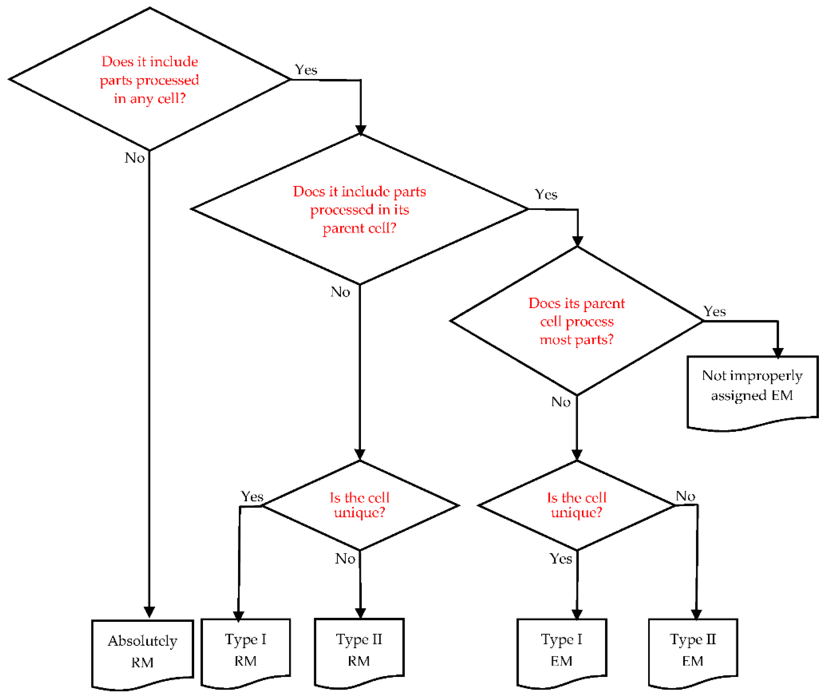
2.3.4. Reassigning Improperly Assigned Exceptional Machines (EMs) and Redundant Machines (RMs)

The CF based on the solution from model 3 and the part family formation may result in an unsatisfactory block diagonal solution due to improperly assigned Ems, which process most parts in other cells, or RMs, which process no parts in their parent cell. Therefore, a subsequent refinement procedure is used to improve the quality of incumbent block diagonal solutions through an inspection by reassigning them to their most appropriate cells if there are any improperly assigned EMs. The reassignment of improperly assigned EMs/RMs can lead to higher GE by decreasing EEs and voids.

The improperly assigned EMs/RMs are categorized as follows:

• An absolute RM which processes no parts in any cell;
• A type I RM which processes most parts in other unique cells except for its parent cell;
• A type II RM which processes most parts in two or more other cells except for its parent cell;
• A type I EM which processes some parts in its parent cell but processes most parts in other unique cells except for its parent cell;
• A type II EM which processes most parts in two or more cells including its parent cell.

To illustrate the types of improperly assigned EMs/RMs, consider a block diagonal matrix as shown in Figure 3. From this matrix, we can observe the set of machine cells, MC₁ = {1, 2, 3}, MC₂ = {4, 5, 6}, and MC₃ = {7, 8}; and the set of part families, PF₁ = {1a, 2b, 3c}, PF₂ = {4a, 5b, 6a}, and PF₃ = {7b, 8c, 9b}. According to the above definition, machines 1, 2, and 3 are type I RM, type II RM, and absolute RM, respectively, and machines 6 and 8 are type I EM and type II EM, respectively.

To determine the type of EM and RM, the following elements need to be evaluated for each machine:

• Its parent cell;
• Cells processing most parts;
• The total number of parts processed; and
• The number of parts processed in its parent cell.

Figure 4 is a flow chart showing the determination of the type of EM or RM for a machine. The reassignment procedure for improperly assigned EMs/RMs is then stated as follows:

• Reassign a type I RM or type I EM to another unique candidate cell;
• Reassign an absolute RM, type II RM or type II EM to the cell with the fewest 1s. If ties occur, reassign them to the cell with the lowest number of machines.
• Remove an absolute RM from the current cell since it does not process any parts under the incumbent cell configuration.

2.3.5. Illustrative Example

The proposed procedures for part assignment and improperly assigned EM/RM reassignment are illustrated with a hypothetical GCF incidence which includes seven machine types, 15 part types, and 35 process plans as shown in

Table 1. Routing information of parts.

Part No.	Process Plan	Machines	Part No.	Process Plan	Machines
1	a	1, 5	9	a	5, 7
	b	1, 3, 4, 6		b	2, 4
2	a	3, 5, 7	10	a	1, 3, 4
	b	2, 3		b	1, 2, 5
3	a	2, 3, 4	11	a	2, 3, 4, 6
4	a	2, 3, 4, 5		b	1, 2, 5
	b	1, 2, 4, 5		c	5, 6, 7
	c	2, 5, 6		d	2, 3, 4, 5, 7
	d	2, 3, 4, 7	12	a	3, 5
5	a	3, 4, 5, 6		b	2, 6
	b	2, 7		c	2, 3, 4
	c	1, 3, 4, 5, 7	13	a	1, 2, 3, 6
6	a	2, 4	14	a	2, 3, 4, 6
	b	1, 3, 6		b	1, 2, 3, 4
7	a	3, 5	15	a	2, 7
	b	4, 5, 7		b	3, 4
8	a	2, 3, 5
	b	4, 6, 7
	c	1, 2, 3, 6

, which lists the routing information of parts. Machine types 3 and 4 have two and one extra copies, respectively. After model 3 is solved under the condition of $p=3$ and $U=4$, the following machine cells are obtained: MC₁ = {1, 3, 6}, MC₂ = {2,4,3}, and MC₃ = {5,7,3,4}.

Once these machine cells are determined, partial assignment steps of parts 1, 2, and 3 are presented in

Table 2. Assignment of parts 1, 2, and 3 to cells.

Part No.	Process Plan	Cells Assigned	Criteria		Part Type	Criteria
			1	2		4	5	6
1	a *	1 *	1 *	2	Type II NEP
		2	2	3
		3 *	1 *	3
	b **	1 **	1 *	0 *
		2	2	1
		3	2	2
2	a **	1	2	2	Type II NNEP
		2	2	2
		3 **	0 *	1 *		0 *	0 *	3 **
	b *	1	1	2
		2 *	0 *	1 *		0 *	0 *	2
		3	1	3
3	a **	1	2	2	Type I SNEP
		2 **	0 *	0 *
		3	1	2

* indicates the candidate process plans and cells and ** indicates the best process plan and cell.

, where the column (1) indicates the number of EEs generated by the process plan assigned to a specific cell. The symbol * indicates the entries corresponding to the candidate process plan and cells selected by the criterion of that step. The symbol ** indicates the entries corresponding to the best process plan and the cell selected by the criterion of the final step. If the best candidate plan is determined, the associated best process plan and cell can be identified by scanning the columns from left to right. After all parts are assigned, no RMs and improperly assigned EMs are found. Figure 5 is the resulting block diagonal solution matrix with a GE of 77.19%.

3. Results

The purpose of the computational experiment performed in this section was two-fold. One aim was to show the effectiveness of our approach compared to the solutions already reported in the literature under the same restrictions as the reference approaches with regard to the number of cells $p$ and cell size $U$; the other was to provide solutions that can be used as benchmarks for comparative testing with different CF solution approaches by finding better alternative solutions that have not been reported in the literature under different values of $p$ and $U$.

The proposed PMP-based hard computing approach has been implemented and tested with two groups of GCF incidences: 26 small to intermediate-sized problem sets available in the literature and three expanded large-sized ones. The large-sized incidences are expanded with values of $p$ which are different from the original ones.

Table 3. Computational results with small to intermediate-sized original incidences. GE: grouping efficacy.

Problem	Problem Size					Reference Algorithm				Proposed Approach
Source	n(q)	m	t	p	U	e	EEs	Voids	GE (%)	e	EEs	Voids	GE (%)	CPU (s)
1. [33]	4	5	11	2	2	9	0	1	90.00	9	0	1	90.00	0.05 a + 0.044 b
2. [35]	6	10	20	2	4	28	2	8	72.22	28	2	8	72.22	0.05 + 0.047
	6(7)	10	20	2	4	27	0	10	72.97	31	0	8	79.49	0.09 + 0.054
3. [65]	20	20	51	5	5	66	1	17	78.31	67	6	16	73.49	0.09 + 0.189
4. [66]	6	6	13	2	3	15	0	3	83.33	15	0	3	83.33	0.05 + 0.044
5. [67]	10	10	27	3	5	47	10	17	57.81	49	12	12	60.66	0.08 + 0.062
	10(13)	15	27	3	5	49	5	20	63.77 c	49	4	21	64.29	0.08 + 0.050
6. [68]	7	14	32	3	3	31	5	6	70.27d	29	5	6	68.57	0.06 + 0.048
7. [69]	10	10	24	3	5	31	1	3	88.24	31	1	3	88.24	0.08 + 0.050
	10(11)	10	24	3	5	33	3	10	69.77	33	1	3	88.89	0.06 + 0.049
8. [70]	8	13	26	3	3	33	2	5	81.58	33	3	4	81.08	0.09 + 0.049
9. [70]	30	30	89	6	7	151	1	48	75.38	150	1	46	76.02	0.11 + 0.065
10. [59]	4	4	8	2	2	8	0	0	100.00	8	0	0	100.00	0.05 + 0.040
	7	10	23	3	3	25	3	2	81.48	23	4	5	67.86	0.06 + 0.045
	11	10	22	4	3	28	3	3	80.65	27	3	4	77.42	0.08 + 0.041
	26	28	71	6	7	124	16	25	72.48	121	15	27	71.62	0.10 + 0.059
11. [71]	8	15	46	2	4	30	1	31	47.54	35	1	26	55.74	0.08 + 0.049
	8	15	46	2	5	NA	NA	NA	NA	33	0	22	60.00	0.07 + 0.048
	8	15	46	3	3	32	1	12	70.45	33	1	9	76.19	0.09 + 0.047
12. [72]	12	20	26	3	5	NA	29	NA	47.06 e	85	31	26	48.65	0.08 + 0.047
13. [72]	14	20	45	3	5	85	24	35	50.83e	85	31	27	48.21	0.09 + 0.051
14. [72]	18	18	59	3	6	116	26	108	40.18 e	116	32	84	42.00	0.09 + 0.054
15. [73]	10(13)	7	13	3	5	22	0	9	70.97	23	1	11	64.71	0.08 + 0.053
16. [74]	6(15)	20	34	3	5	49	0	52	48.51 e	49	0	51	49.00	0.08 + 0.048
17. [75]	6	8	14	2	3	21	1	4	80.00	22	1	3	84.00	0.05 + 0.046
18. [75]	5	7	11	2	3	15	0	3	83.33	17	1	1	88.89	0.05 + 0.047
19. [75]	10(14)	16	31	2	7	68	8	52	50.00	68	1	45	59.29	0.08 + 0.050
20. [76]	10(16)	20	35	2	10	77	0	87	46.95	77	4	79	46.79	0.09 + 0.049
21. [77]	9	8	20	2	6	28	2	13	63.41	28	2	10	68.42	0.08 + 0.046
22. [78]	30	70	149	2	15	NA	NA	NA	NA	477	132	717	28.89	0.15 + 0.079
	30	70	149	3	10	NA	NA	NA	NA	478	193	415	31.91	0.28 + 0.082
	30	70	149	4	8	NA	NA	NA	NA	477	219	290	33.64	0.17 + 0.081
	30	70	149	5	6	NA	NA	NA	NA	478	249	192	34.18	0.16 + 0.081
23. [51]	30	35	82	4	8	224	52	92	54.43	229	52	86	56.19	0.18 + 0.067
	30	35	100	5	7	NA	NA	NA	NA	233	58	38	64.58	0.13 + 0.066
24. [51]	40	45	100	6	8	263	39	86	64.18	263	37	85	64.94	0.19 + 0.076
	40	45	100	7	7	NA	NA	NA	NA	266	42	36	74.17	0.26 + 0.069
25. [51]	55	60	124	8	9	402	50	62	75.86	411	50	53	77.80	0.27 + 0.076
26. [62]	8	20	27	3	4	60	10	2	80.65	60	10	2	80.65	0.07 + 0.051

(^a) Running time implementing model 3. (^b) Running time assigning parts and reassigning improperly assigned EMs/RMs. (^c) The best solution reported in [69]. (^d) The best solution reported in [79]. (^e) The best solution reported in [61].

and

Table 4. Computational results with double-expanded large-size incidences.

Original Problem	Expanded Problem Size					Proposed Approach
	n(q)	m	t	p	U	e	EEs	Voids	GE (%)	CPU (s)
1. [70]	60	60	178	12	7	302	2	90	76.53	0.28 + 0.085
2. [78]	60	140	298	10	6	956	502	386	33.83	0.89 + 0.129
3. [51]	60	70	164	10	7	466	116	76	64.58	0.58 + 0.095
4. [51]	80	90	200	14	7	533	81	70	74.96	0.77 + 0.101
5. [51]	110	120	248	16	9	822	100	106	77.80	0.63 + 0.121

show a total of 39 test incidences for 26 small to intermediate-sized original problems and a total of five expanded test incidences for three large-sized original problems, respectively.

The former incidences are used for comparative purposes along with the results obtained by the reference approaches; the latter incidences are used to show the effectiveness of our approach in solving large-sized GCF incidences. The double-expanded large-size incidences have been produced by following Adil et al.’s data expansion scheme [80], which duplicates rows and columns of an existing intermediate-sized binary PMIM instead of using randomly generated data sets.

For the original problems 6, 11, 22, 23, and 24 in Table 3, extra incidences have been tested for values of $p$ and $U$ different from those used the in the original problems. Some of the original data sets include information on the operation sequences and/or production volumes of parts. Those data sets are slightly changed so that the resulting routing data or PMIMs are suited for the 0–1 GCF problem format. For problem 5, process plans b and c of part type 2 are merged into an identical process plan since they require the same tools. For problems 17 and 19, process plan c of part type 1 has been deleted since it requires the same machines as process plan b. All the GCF incidences and block diagonal solution matrices are available upon request.

Model 3 has been solved using the LINGO 16.0 solver on an ASUS laptop computer including an Intel Core i7-9750H processor running at 2.6 GHz with 16 GB RAM under the Windows 10 operating system. The procedures for part assignment and improperly assigned EM/RM reassignment were coded in C + + and implemented using the Visual Studio 2015. The execution times taken to implement all the reference CF methods selected for comparative purposes will not be reported since each incidence selected in our experiment was solved using different machines and compilers; only the execution time taken to implement our approach is reported for future comparison.

4. Discussion

In Table 3, the bold-faced GEs indicate the best GEs obtained from the corresponding reference approach and proposed PMP hard computing approach. Of these 39 test incidences, the best published values of GE under the corresponding conditions of $p$ and $U$ for four incidences of problem 22 and three extra test incidences of problems 11, 23, and 24 have not been reported in the literature. Therefore, these instances are not used for performance comparison between the reference approaches and the proposed PMP approach and are reported only for the purpose of future comparison.

According to the computational result presented in Table 3, for six incidences (6/32 = 18.8%) of problems 1, 2, 4, 7, 10, and 26, both approaches yield the same GEs. For nine incidences (9/32 = 28.1%) of problems 3, 6, 8, 10, 13, 15, and 20, the reference approaches yield better GEs than the PMP approach. For 17 incidences (17/32 = 53.1%) of problems 2, 5, 7, 9, 11, 12, 14, 16, 17, 18, 19, 21, 23, 24, and 25, the PMP approach yields better GEs than the reference approaches. In summary, the proposed PMP hard computing approach absolutely outperforms the existing soft or hard computing approaches by 53.1% for the small to intermediate GCF incidences available in the literature. Furthermore, the proposed PMP hard computing approach finds better alternative solutions which were not found by the reference approaches with values of $p$ and $U$ which were different from the original problems 11, 23, and 24.

Regarding the computing time required to implement model 3, the proposed PMP hard computing approach reached the global optimum within 0.3 s even for a large incidence of 24 including 3025 binary variables. The execution times required to implement subsequent procedures for part assignment and improperly assigned EM/RM reassignment were also negligibly small since those procedures were terminated within 0.1 s for all incidences.

The proposed PMP hard computing approach has been applied to larger GCF incidences in order to show how efficiently the PMP hard computing approach solves large-sized GCF incidences. To the best of our knowledge, problem 24 is the largest open GCF incidence that is available in the literature and therefore can be used for comparative purposes with different CF solution approaches. Some authors [61,81] tested the efficiency of their CF solution approaches with randomly generated incidences in order to show the efficiency of their methods for large-sized incidences. However, they did not provide solutions that show an explicit configuration of machine cells and associated part families. As a result, the best published values of GE for those incidences are not available for benchmark testing with such randomly generated incidences.

To show how efficiently the proposed PMP hard computing approach solves even larger GCF incidences, we have chosen to double-expand some original large incidences instead of using randomly generated incidences. For this purpose, problems 8 and 21 to 24 were selected and expanded. A typical strategy used to randomly generate large-sized matrices is to create an ideal block diagonal structure first and then destroy it gradually by using random flips. The random flipping of the original GCF matrices is performed to change 1s in the diagonal blocks into zeros and zeros in the off-diagonal blocks into 1s [34]. The more flipped the expanded matrices, the less random they become. However, the large GCF incidences generated through double-expansion in our computational experiment are not randomly flipped, meaning that the resulting matrices do not approach completely random ones. By avoiding random flips over the expanded matrices, we can test both the efficiency and robustness of the proposed PMP approach. The only element randomly scrambled is the order of part numbers.

Table 4 shows the double-expanded incidences and computational results with those incidences. The numbers of machines of expanded incidences vary from 60 to 110, and the numbers of binary variables therefore vary from 3600 to 12,100. As far as the author knows, few mathematical models have been implemented to use a hard computing approach to optimally solve large-sized GCF incidences with such a large number of binary variables. According to Table 4, model 3 reaches the global optimum for all the expanded incidences within one second. Subsequent procedures for part assignment and improperly assigned EM/RM reassignment were terminated within 0.2 s. Clearly, this shows the computational efficiency of the proposed PMP hard computing approach for large-sized GCF problems. Furthermore, except for incidence 2, which was double-expanded for problem 21, the remaining double-expanded incidences even yielded better GEs than the original incidence before double-expansion. This reveals the robustness of the proposed PMP approach when applied to large-sized GCF problems.

5. Conclusions

In this paper, we have proposed an effective hard computing technique to solve large-sized GCF incidences to the global optimum within a short computation time. The distinctive contributions of this paper are summarized as follows:

• Two new linear 0–1 mathematical models have been formulated to solve the GCF problem: an exact model to directly maximize the GE and a PMP-type model to indirectly maximize the GE;
• It seems still to be very difficult to use a hard computing approach to optimally solve large-sized GCF incidences of an exact mathematical model optimizing the objective function directly.
• The PMP-type model, as an alternative to optimizing the objective function of GCF indirectly, can use hard computing techniques to solve large-sized GCF incidences optimally in a very short computation time. Even a large GCF incidence containing 12,100 binary variables can be solved within only one second to the global optimum, and the machine cells can be identified.
• The computation time for subsequent part assignment procedures finding the associated part families and refinement steps and reassigning improperly assigned EMs/RMs is also negligibly small, even if some soft computing heuristics can work faster, as shown by Goldengorin et al. [34].
• The solution quality based on the proposed hard computing approach compares favorably to existing GCF solution approaches.
• The GCF incidences collected in our computation experiment can be used as a standard data set for subsequent benchmark tests in the future.

A limitation of the paper should be addressed. Unlike Danilovic & Ilic’s part assignment rule [50], the part assignment procedure proposed in this paper does not guarantee the optimal part assignment since it is heuristic. The solution quality due to the assignment of a part depends on the assignment of other parts. Therefore, establishing sufficient conditions for optimal part assignment in the GCF problem will be a very attractive future research issue.

References

1. Burbidge, J.L. The new approach to production. Prod. Eng. 1961, 40, 769–794. [Google Scholar] [CrossRef]
2. Wemmerlöv, U.; Johnson, D.J. Empirical findings on manufacturing cell design. Int. J. Prod. Res. 2000, 38, 481–507. [Google Scholar] [CrossRef]
3. Ballakur, A.; Steudel, H.J. A within–cell utilization based heuristic for designing cellular manufacturing systems. Int. J. Prod. Res. 1987, 25, 639–655. [Google Scholar] [CrossRef]
4. Batsyn, M.V.; Batsyna, E.K.; Bychkov, I.S. On NP-completeness of the cell formation problem. Int. J. Prod. Res. 2019, in press. [Google Scholar] [CrossRef]
5. Papaioannou, G.; Wilson, J.M. The evolution of cell formation problem methodologies based on recent studies (1997–2008): Review and directions for future research. Eur. J. Oper. Res. 2010, 206, 509–521. [Google Scholar] [CrossRef] [Green Version]
6. Lozano, S.; Guerrero, F.; Eguia, I.; Onieva, L. Cell design and loading in the presence of alternative routing. Int. J. Prod. Res. 1999, 37, 3289–3304. [Google Scholar] [CrossRef]
7. Islam, K.M.S.; Sarker, B.R. A similarity coefficient measure and machine-parts grouping in cellular manufacturing systems. Int. J. Prod. Res. 2000, 38, 699–720. [Google Scholar] [CrossRef]
8. Heragu, S.S.; Chen, J.S. Optimal solution of cellular manufacturing system design: Benders’ decomposition approach. Eur. J. Oper. Res. 1998, 107, 175–192. [Google Scholar] [CrossRef]
9. Borrero, J.S.; Gillen, C.; Prokopyev, O.A. Fractional 0–1 programming: Applications and algorithms. J. Glob. Optim. 2017, 69, 255–282. [Google Scholar] [CrossRef]
10. Kumar, C.S.; Chandrasekharan, M.P. Grouping efficacy: A quantitative criterion for goodness of block diagonal forms of binary matrices in group technology. Int. J. Prod. Res. 1990, 28, 233–243. [Google Scholar] [CrossRef]
11. Elbenani, B.; Ferland, J.A. Cell formation problem solved exactly with the Dinkelbach algorithm. CIRRET 2012, 7, 1–14. [Google Scholar]
12. Elbenani, B.; Ferland, J.A. An exact method for solving the manufacturing cell formation problem. Int. J. Prod. Res. 2012, 50, 4038–4045. [Google Scholar] [CrossRef]
13. Bychkov, I.; Batsyn, M.; Pardalos, P.M. Exact model for the cell formation problem. Optim. Lett. 2014, 8, 2203–2210. [Google Scholar] [CrossRef]
14. Brusco, M.J. An exact algorithm for maximizing grouping efficacy in part-machine clustering. IIE Trans. 2015, 47, 653–671. [Google Scholar] [CrossRef]
15. Pinheiro, R.G.S.; Martins, I.C.; Protti, F.; Ochi, L.S.; Simonetti, L.G.; Subramanian, A. On solving manufacturing cell formation via bicluster editing. Eur. J. Oper. Res. 2016, 254, 769–779. [Google Scholar] [CrossRef] [Green Version]
16. Utkina, I.; Batsyn, M.V.; Batsyna, E.K. A branch and bound algorithm for a fractional 0-1 programming problem. In Discrete Optimization and Operations Research; Kochetov, Y., Khachay, M., Beresnev, V., Nurminski, E., Pardalos, P., Eds.; Lecture Notes in Computer Science; Springer: New York, NY, USA, 2016; Volume 9869, pp. 244–255. [Google Scholar]
17. Bychkov, I.; Batsyn, M. An efficient exact model for the cell formation problem with a variable number of production cells. Comput. Oper. Res. 2018, 91, 112–120. [Google Scholar] [CrossRef] [Green Version]
18. Utkina, I.; Batsyn, M.V.; Batsyna, E.K. A branch-and-bound algorithm for the cell formation problem. Int. J. Prod. Res. 2018, 56, 3262–3273. [Google Scholar] [CrossRef]
19. Goncalves, J.F.; Resende, M.G.C. An evolutionary algorithm for manufacturing cell formation. Comput. Ind. Eng. 2004, 47, 247–273. [Google Scholar] [CrossRef]
20. Hakimi, S.L. Optimum location of switching centers and the absolute centers and medians of a graph. Oper. Res. 1964, 12, 450–459. [Google Scholar] [CrossRef]
21. Hakimi, S.L. Optimum distribution of switching centers and some graph related theoretic problems. Oper. Res. 1965, 13, 462–475. [Google Scholar] [CrossRef]
22. Shi, J.; Zheng, X.; Jiao, B.; Wang, R. Multi-scenario cooperative evolutionary algorithm for the β-Robust p-median problem with demand uncertainty. Appl. Sci. 2019, 9, 4174. [Google Scholar] [CrossRef] [Green Version]
23. ReVelle, C.S.; Swain, R.W. Central Facilities location. Geogr. Anal. 1970, 2, 30–42. [Google Scholar] [CrossRef]
24. Balinski, M. Integer programming: Methods, uses, computations. Manag. Sci. 1965, 12, 253–313. [Google Scholar] [CrossRef]
25. Efroymson, M.A.; Ray, T.L. A branch-bound algorithm for plant location. Oper. Res. 1966, 14, 361–368. [Google Scholar] [CrossRef]
26. Church, R.L. COBRA: A new formulation of the classic p-median location problem. Ann. Oper. Res. 2003, 122, 103–120. [Google Scholar] [CrossRef]
27. Goldengorin, B.; Ghosh, D.; Sierksma, G. Branch and peg algorithms for the simple plant location problem. Comput. Oper. Res. 2003, 30, 967–981. [Google Scholar] [CrossRef] [Green Version]
28. Goldengorin, B.; Tijssen, G.A.; Ghosh, D.; Sierksma, G. Solving the simple plant location problems using a data correcting approach. J. Global Optim. 2003, 25, 377–406. [Google Scholar] [CrossRef]
29. Church, R.L. BEAMR: An exact and approximate model for the p-median problem. Comput. Oper. Res. 2008, 35, 417–426. [Google Scholar] [CrossRef]
30. Elloumi, S. A tighter formulation of the p-median problem. J. Glob. Optim. 2010, 19, 69–83. [Google Scholar] [CrossRef]
31. García, S.; Labbé, M.; Marín, A. Solving large p-median problems with a radius formulation. INFORMS J. Comput. 2011, 23, 546–556. [Google Scholar] [CrossRef]
32. Kusiak, A. The part families problem in flexible manufacturing systems. Ann. Oper. Res. 1985, 3, 279–300. [Google Scholar] [CrossRef]
33. Kusiak, A. The Generalized group technology concept. Int. J. Prod. Res. 1987, 25, 561–569. [Google Scholar] [CrossRef]
34. Goldengorin, B.; Krushinsky, D.; Slomp, J. Flexible PMP approach for large-size cell formation. Oper. Res. 2012, 60, 1157–1166. [Google Scholar] [CrossRef]
35. Sankran, S.; Kasilingam, R.G. An integrated approach to cell formation and part routing in group technology. Eng. Optim. 1990, 16, 235–245. [Google Scholar] [CrossRef]
36. Kaparthi, S.; Suresh, N.C. Performance of selected part-machine grouping techniques for data sets of wide ranging sizes and imperfection. Decis. Sci. 1994, 25, 515–539. [Google Scholar] [CrossRef]
37. Lee, H.; Garcia-Diaz, A. Network flow procedures for the analysis of cellular manufacturing systems. IIE Trans. 1996, 28, 333–345. [Google Scholar] [CrossRef]
38. Viswanathan, S. A new approach for solving the p-median problem in group technology. Int. J. Prod. Res. 1996, 34, 2691–2700. [Google Scholar] [CrossRef]
39. Deutsch, S.J.; Freeman, S.F.; Helander, M. Manufacturing cell formation using an improved p-median model. Comput. Ind. Eng. 1998, 34, 135–146. [Google Scholar] [CrossRef]
40. Won, Y. New p-median approach to cell formation with alternative process plans. Int. J. Prod. Res. 2000, 38, 229–240. [Google Scholar] [CrossRef]
41. Won, Y. Two-phase approach to GT cell formation using efficient p-median formulations. Int. J. Prod. Res. 2000, 38, 1601–1613. [Google Scholar] [CrossRef]
42. Won, Y.; Lee, K.C. Modified p-median approach for efficient GT cell formation. Comput. Ind. Eng. 2004, 46, 495–510. [Google Scholar] [CrossRef]
43. Ashayeri, J.; Heuts, R.; Tammel, B. A modified simple heuristic for the p-median problem, with facilities design applications. Robot. CIM Int. Manuf. 2005, 21, 451–464. [Google Scholar] [CrossRef]
44. Won, Y.; Currie, K.R. An effective p-median model considering production factors in machine cell/part family formation. J. Manuf. Syst. 2006, 25, 58–64. [Google Scholar] [CrossRef]
45. Süer, G.A.; Huang, J.H.; Maddisetty, S. Design of dedicated, shared and remainder cells in a probabilistic demand environment. Int. J. Prod. Res. 2010, 48, 5613–5646. [Google Scholar] [CrossRef]
46. Egilmez, G.; Süer, G.A.; Huang, J. Stochastic cellular manufacturing system design subject to maximum acceptable risk level. Comput. Ind. Eng. 2012, 63, 842–854. [Google Scholar] [CrossRef]
47. Egilmez, G.; Süer, G.A. The impact of risk on the integrated cellular design and control. Int. J. Prod. Res. 2014, 52, 1455–1478. [Google Scholar] [CrossRef]
48. Won, Y.; Logendran, R. Effective two-phase p-median approach for the balanced cell formation in the design of cellular manufacturing system. Int. J. Prod. Res. 2015, 53, 2730–2750. [Google Scholar] [CrossRef]
49. Alhawari, O.; Süer, G. Modified p-median model with minimum threshold for average family similarity. Procedia Manuf. 2019, 39, 1048–1056. [Google Scholar] [CrossRef]
50. Danilovic, M.; Ilic, O. A novel hybrid algorithm for manufacturing cell formation problem. Expert Syst. Appl. 2019, 135, 327–350. [Google Scholar] [CrossRef]
51. Kao, Y.; Chen, C.C. Automatic clustering for generalised cell formation using a hybrid particle swarm optimisation. Int. J. Prod. Res. 2014, 52, 3466–3484. [Google Scholar] [CrossRef]
52. Riccardo, M.; Riccardo, A.; Marco, B. Similarity-based cluster analysis for the cell formation problem. In Operations Management Research and Cellular Manufacturing Systems: Innovative Methods and Approaches; Modrák, V., Pandian, R.S., Eds.; IGI Global: Hershey, PA, USA, 2012; pp. 140–163. [Google Scholar]
53. Li, X.; Baki, M.; Aneja, Y. An ant colony optimization metaheuristic for machine-part cell formation problems. Comput. Oper. Res. 2010, 37, 2071–2081. [Google Scholar] [CrossRef]
54. Vin, E.; Delchambre, A. Generalized cell formation: Iterative versus simultaneous resolution with grouping genetic algorithm. J. Intell. Manuf. 2014, 25, 1113–1124. [Google Scholar] [CrossRef]
55. Sarker, B.R. Measures of grouping efficiency in cellular manufacturing systems. Eur. J. Oper. Res. 2001, 130, 588–611. [Google Scholar] [CrossRef]
56. Sarker, B.R.; Khan, M. A comparison of existing grouping efficiency measures and a new weighted grouping efficiency measure. IIE Trans. 2001, 33, 11–27. [Google Scholar] [CrossRef]
57. Mahdavi, I.; Javadi, B.; Fallah-Alipour, K.; Slomp, J. Designing a new mathematical model for cellular manufacturing system based on cell utilization. Appl. Math. Comput. 2007, 190, 662–670. [Google Scholar] [CrossRef]
58. Paydar, M.M.; Saidi-Mehrabad, M. A hybrid genetic-variable neighborhood search algorithm for the cell formation problem based on grouping efficacy. Comput. Oper. Res. 2013, 40, 980–990. [Google Scholar] [CrossRef]
59. Won, Y.; Kim, S. Multiple criteria clustering algorithm for solving the group technology problem with multiple process routings. Comput. Ind. Eng. 1997, 32, 207–220. [Google Scholar] [CrossRef]
60. Mukattash, A.M.; Adil, M.B.; Tahboub, K.K. Heuristic approaches for part assignment in cell formation. Comput. Ind. Eng. 2002, 42, 327–341. [Google Scholar] [CrossRef]
61. Wu, T.H.; Chung, S.H.; Chang, C.C. Hybrid simulated annealing algorithm with mutation operator to the cell formation problem with alternative process routings. Expert Syst. Appl. 2009, 36, 3652–3661. [Google Scholar] [CrossRef]
62. Shiyasa, C.R.; Pillaia, V.M. Cellular manufacturing system design using grouping efficacy-based genetic algorithm. Int. J. Prod. Res. 2014, 52, 3504–3517. [Google Scholar] [CrossRef]
63. Won, Y. P-median approach for the large-size multi-objective generalized cell formation. Korean Manag. Sci. Rev. 2018, 35, 35–55. [Google Scholar] [CrossRef]
64. Al-Zawahreha, A.; Dahmanib, N.; Alethem, K.A.; Mukattash, A. Sensitivity analysis of the impact of part assignment in cellular manufacturing systems. Decis. Sci. Lett. 2019, 8, 109–120. [Google Scholar] [CrossRef]
65. Nagi, R.; Harhalakis, G.; Proth, J. Multiple routings and capacity consideration in group technology applications. Int. J. Prod. Res. 1990, 28, 2243–2257. [Google Scholar] [CrossRef]
66. Moon, Y.B.; Chi, S.C. Generalized part family formation using neural network techniques. J. Manuf. Syst. 1992, 11, 149–159. [Google Scholar] [CrossRef]
67. Kasilingam, R.G.; Lashkari, R.S. Cell formation in the presence of alternate process plans in flexible manufacturing systems. Prod. Plan. Control. 1991, 2, 135–141. [Google Scholar] [CrossRef]
68. Logendran, R.; Ramakrishna, P.; Sriskandarajah, C. Tabu search-based heuristics for cellular manufacturing systems in the presence of alternative process plans. Int. J. Prod. Res. 1994, 32, 273–297. [Google Scholar] [CrossRef]
69. Adil, G.K.; Rajamani, D.; Strong, D. Cell formation considering alternate routeings. Int. J. Prod. Res. 1996, 34, 1361–1380. [Google Scholar] [CrossRef]
70. Lee, M.K.; Luong, H.S.; Abhary, K. A genetic algorithm based cell design considering alternative routing. Comput. Integr. Manuf. 1997, 10, 93–107. [Google Scholar] [CrossRef]
71. Han, J. Formation of Part and Machine Cells with Consideration of Alternative Machines. Master’s Thesis, Ohio University, Athens, OH, USA, 1998. [Google Scholar]
72. Sofianopoulou, S. Manufacturing cells design with alternative process plans and/or replicate machines. Int. J. Prod. Res. 1999, 37, 707–720. [Google Scholar] [CrossRef]
73. Gen, M.; Cheng, R. Manufacturing cell design. In Genetic Algorithms and Engineering Optimization; John Wiley & Sons: New York, NY, USA, 2000; pp. 390–450. [Google Scholar]
74. Aktürk, M.S.; Turkcan, A. Cellular manufacturing system design using a holonistic approach. Int. J. Prod. Res. 2000, 38, 2327–2347. [Google Scholar] [CrossRef]
75. Yin, Y.; Yasuda, K. Manufacturing cells’ design in consideration of various production factors. Int. J. Prod. Res. 2002, 40, 885–906. [Google Scholar] [CrossRef]
76. Solimanpur, M.; Vrat, P.; Shankar, R. A multi-objective genetic algorithm approach to the design of cellular manufacturing systems. Int. J. Prod. Res. 2004, 42, 1419–1441. [Google Scholar] [CrossRef]
77. Bhide, P.; Bhandwale, A.; Kesavadas, T. Cell formation using multiple process plans. J. Intell. Manuf. 2005, 16, 53–65. [Google Scholar] [CrossRef]
78. Hu, L.; Yasuda, K. Minimising material handling cost in cell formation with alternative processing routes by grouping genetic algorithm. Int. J. Prod. Res. 2006, 44, 2133–2167. [Google Scholar] [CrossRef]
79. Hwang, H.; Ree, P. Routes selection for the cell formation problem with alternative part process plans. Comput. Ind. Eng. 1996, 30, 423–431. [Google Scholar] [CrossRef]
80. Adil, G.K.; Rajamani, D.; Strong, D. Assignment allocation and simulated annealing algorithms for cell formation. IIE Trans. 1997, 29, 53–67. [Google Scholar] [CrossRef]
81. Wu, T.H.; Chen, J.F.; Yeh, J.Y. A decomposition approach to the cell formation problem with alternative process plans. Int. J. Adv. Manuf. Technol. 2004, 24, 834–840. [Google Scholar] [CrossRef]
Figure 1. (a) Initial generalized part–machine incidence matrix (PMIM=; (b) block diagonal solution matrix.
Applsci 10 03478 g001
Figure 2. Flow chart identifying the category of part. SNEP: strongly nonexceptional part; NNEP: neutrally nonexceptional part; WEP: weakly exceptionally part; NEP: neutrally exceptional part.
Applsci 10 03478 g002
Figure 3. A block diagonal matrix for identifying the type of exceptional machines (EMs)/redundant machines (RMs).
Applsci 10 03478 g003
Figure 4. Flow chart identifying the type of EM and RM.
Applsci 10 03478 g004
Figure 5. Block diagonal solution to the hypothetical example.
Applsci 10 03478 g005