Olive Oils Classification via Laser-Induced Breakdown Spectroscopy

Abstract

The classification of olive oils and the authentication of their geographic origin are important issues for public health and for the olive oil market and related industry. The development of fast, easy to use, suitable for on-line, in-situ and remote operation techniques for olive oils classification is of high interest. In the present work, 36 olive oils from different places in Crete, Greece, are studied using a laser-based technique, Laser-Induced Breakdown Spectroscopy (LIBS), assisted by machine learning algorithms, aiming to classify them in terms of their geographical origin. The excellent classification results obtained demonstrate the great potential of LIBS, which is further extended by the use of machine learning.

1. Introduction

Olive oil is a key element of the Mediterranean diet because of its excellent nutritional and organoleptic properties. Extra Virgin Olive Oils (EVOOs), in particular, usually attain much higher price than other types of vegetable oils; this difference resulted from the increased demand of the markets and the preferences of the consumers, the latter being oriented during recent years, progressively, towards higher quality and more healthy food products and ingredients. Inevitably, this situation makes EVOOs more prone to adulteration by other lower cost vegetable oils (as e.g., pomace oil). In addition, when the olive oil of a region is recognized for its unique properties (as e.g., taste, odor, color, etc.) and assessed for that by the specialists and the consumers, its designation of origin and/or geographical indication is becoming finally a brand name, giving added value and therefore resulting in higher market prices. Thus, Protected Designation of Origin (PDO) and/or Protected Geographical Indication (PGI) protocols can significantly differentiate the different types of olive oils [1,2,3,4]. In that view, the control of the authenticity of foodstuff is essential and necessary for the fair trade between the producers and the consumers, and there are several national (e.g., Hellenic Food Authority-EFET in Greece) and international (e.g., European Commission) organizations in charge to set and control the frameworks about the allowed concentration of the different food ingredients while they are often responsible to prepare the necessary legislation in order to preserve the PDO and the PGI of food. Then, according to this legislation, food’s categorization, which is based on its variety and designation of origin, is set as a criterion of their authenticity and quality.

During the last twenty years, there have been several common methodologies for olive oil testing, which are mainly used for assessing the oil’s suitability as an edible product (e.g., by labeling it as extra virgin, virgin, lampante, etc.), for determining the amounts of substances which are related with its quality, such as the phenolic content and stigmatadienes [5], and for determining its regional provenance. The most standard and common methods employed are liquid and gas chromatographic techniques. However, they require significant laboratory workload for the full characterization of an olive oil sample; despite the high accuracy and excellent results they offer, there is need for new techniques that can alleviate the workload associated with their use. In addition, some important issues that need to be resolved are the identification of geographical origin, and/or the classification of olive oils based on their acidity, etc. As an alternative to the chromatographic techniques, different spectroscopic techniques have been proposed and applied for the analysis of olive oils, with different degree of success, such as NMR spectroscopy [6,7], FT-IR spectroscopy [8,9], Raman spectroscopy [10,11,12] and, recently, Laser-Induced Breakdown Spectroscopy (LIBS) [13,14,15]. LIBS is a laser based analytical technique that uses an intense enough laser beam to induce a dielectric breakdown in a sample or on its surface [16,17]. The result is the formation of a spark, i.e., a plasma, which contains atoms and small (mainly diatomic) molecules (that can be excited or not), ions and electrons. The so produced plasma lives, in general, for a short time (e.g., up to some tens/hundreds of μs), depending on the material, while during this time, it emits some characteristic spectral radiations arising from its different excited constituents and the physical processes occurring in the hot plasma. The spectral analysis of the plasma radiation contains information about the sample’s elemental composition, being a kind of spectral fingerprint. The collection of such LIBS spectra is rapid, does not require any previous time-consuming preparation of the sample and it can be performed on-line, in situ and even remotely. Among the different advantages of the LIBS technique is its ability to analyze any state of matter (i.e., solids, gases, liquids, metals or dielectrics).

Since the elemental composition of olive oil is mainly of carbon, hydrogen and oxygen, the corresponding olive oil LIBS spectra are expected to exhibit spectral features related to these elements with some intensity differences [17]. Therefore, the classification/discrimination of olive oil, based only on such LIBS spectra, is not very useful or at least extremely difficult. To overcome this difficulty, machine learning techniques can be employed to unravel any valuable information contained in these LIBS spectra. Machine learning algorithms can perform tasks suitable for categorizing/classifying data into desired and distinct classes. These algorithms have been widely applied on LIBS data [18], for classification of steel materials [19], for the classification/identification of polymeric samples [20,21], for biomedical and agricultural applications [22,23,24] and for food analysis [25,26].

LIBS analysis of olive oils for classification purposes has been reported up to very recently by few groups. Among them, Caceres et al. were the first using LIBS combined with artificial neural networks to study various types of olive oils and report successful classification of the oils they examined in terms of their geographical origin. Shortly after, in another work [14] using the ratio of C(I)–247.8 nm to the C₂ band at 516.6 nm, some vegetable oils were successfully classified by LIBS in terms of their saturated fatty acid content. More recently, in another study [15], LIBS combined with some machine learning algorithms was used for the classification of some olive oils in terms of their geographical origin and acidity content. It was the first time, to the best of our knowledge, that LIBS assisted by different machine learning algorithms was used for such classification. The reported classification accuracies were quite successful however a limited number of samples were used for the proof-of-concept of the proposed experimental approach. In the present work, a more extended study is performed, employing Laser-Induced Breakdown Spectroscopy assisted by some machine learning techniques for the classification/discrimination of a much larger number of olive oils (33 EVOOs and 3 VOOs), based on their geographical origin. The present olive oils correspond to a more geographically representative data set and they have been collected following specific protocols.

2. Materials and Methods

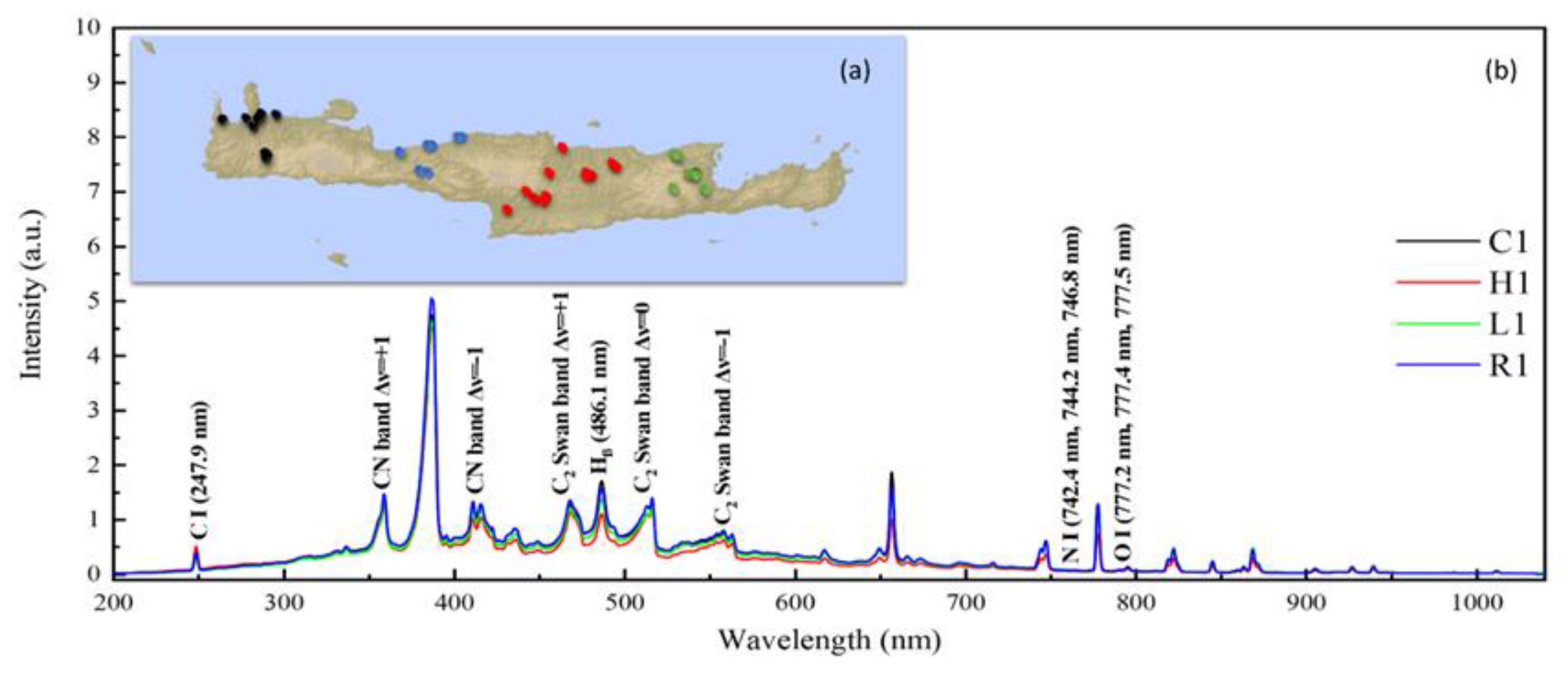
2.1. The Olive Oil Samples

The studied olive oils were classified as EVOOs (33) and VOOs (3) according to free fatty acid and peroxide values [27], and they were collected directly from the producers following specific and strict protocols, from different areas of the island of Crete, Greece. The geographical distribution of the studied olive oils is shown in Figure 1a. The great majority of the studied olive oils (i.e., 33 samples) belong to the Koroneiki cultivar, while 3 samples were a mixture of Koroneiki and Tsounati cultivars. They originated from the following geographical areas of Crete: Chania (9 samples, denoted as C1–C9), Rethymnon (8 samples, R1–R8), Heraklion (12 samples, H1–H12) and Lasithi (7 samples, L1–L7). All samples, after their collection, were stored in dark-colored glass bottles and were kept at a temperature of 2–4 °C. Prior to the laser measurements, the oil samples were left at room temperature for about four hours. More detailed information about the samples is presented in Table S1 in the Supplementary Material section.

2.2. LIBS Setup

For the needs of the experiments, 2 ml of each sample were placed in small shallow uncovered glass recipients with diameters of 2.5 cm (i.e., petri dishes), allowing access of the focused laser beam on their free surface in order to induce a spark, i.e., a plasma. For the creation of the plasma the focused laser beam of a 5 ns Q-switched Nd: YAG laser (Quanta-Ray INDI, Spectra Physics) operating at its fundamental frequency at 1064 nm was used. The laser beam was focused on the olive oil sample surface using a 100 mm focal length quartz lens. The energy of the laser pulses employed was about 80–90 mJ. The laser focusing conditions and the laser energy were optimized in order to provide a sufficiently good signal-to-noise-ratio (SNR) and avoid important splashing, which inevitably occurred. The emission from the plasma was collected via a quartz lens and fed into a quartz optical fiber bundle, the latter being coupled to the entrance slit of a 75 mm focal length spectrograph (Avantes, AvaSpec-2048-USB2). The spectrograph had a 300 lines/mm grating and its detector was 2048-pixel CCD (see e.g., Figure S1).

The spectroscopic system allowed for the observation of the spectral range from 200 to 1100 nm with a resolution of 0.44 nm/pixel. The measurements were performed using a time delay (t_d) of 1.28 μs, and an integration time (t_w) of 1.05 ms for the CCD detector, which were the minimum values allowed by the electronic hardware of the instrument. For the measurements, every laser shot induced a plasma, while ten successive laser shots were averaged corresponding to one LIBS measurement. Then, up to 100 such LIBS spectra were collected, from different places of the free surface, and were used for the statistical analysis. However, after several experiments, it was determined that no significant improvement of the statistical analysis accuracies was occurring for more than 15–20 LIBS spectra. As a result, it was decided to use only 30 such independent LIBS measurements for the algorithms’ training.

2.3. Data Analysis

For the analysis of the LIBS spectroscopic data collected from the different olive oils, some machine learning techniques were selected, employed and assessed for this kind of input data set, i.e., LIBS spectral data, using the Python library Scikit-learn [28]. Among the different machine learning algorithms applied, were the Principal Component Analysis (PCA) [29], the Linear Discriminant Analysis (LDA) [30], the k-Nearest Neighbors (k-NN) [31] and the Support Vector Classifiers (SVC) [32].

Briefly, the PCA is an unsupervised machine learning technique well known for its efficiency for dimensionality reduction of large data sets while maintaining most of the initial information. To accomplish this task, PCA uses an orthogonal transformation to convert the initial dataset (i.e., the LIBS spectra here) into a set of uncorrelated variables, namely the Principal Components (PCs), where the first principal component, PC1, has the largest possible variance, and each succeeding component, in turn, has the highest possible variance under the constraint that it is orthogonal to the preceding components. These variables can be plotted and, thus, the original dataset can be visualized based on its variance, providing a simple and straightforward approach for the visual inspection of the classes.

Oppositely to the PCA algorithm, LDA is a supervised algorithm. It is commonly used for dimensionality reduction problems as a pre-processing step for machine learning applications and for visualization purposes as well. As a supervised learning technique, it can be used as a classification algorithm, as well. LDA maximizes the ratio of the between-class variance over the within-class variance through a classifier with a linear decision boundary, generated by fitting class conditional densities to the data and using Bayes’ theorem. The LDA model fits a Gaussian probability density to each class with the assumption that all classes share the same variance–covariance matrix.

In addition to the LDA approach, two more supervised algorithms were employed in this work for the olive oils classification: the k-NN and SVC algorithms. In both k-NN and SVC classifications, the output is a class membership. In particular, in k-NN, an object is classified by a majority vote of its neighbors, with the object being assigned to the most common class among its k-nearest neighbors. In a different view, in SVC, each data point is viewed as a vector in a n-dimensional space with the value of each feature being the value of a coordinate. Then, SVC classification is performed by finding a hyper-plane that best differentiates the different classes.

The supervised algorithms (LDA, k-NN and SVC) were applied both on raw and on pre-processed data. The latter ones were obtained by pre-processing using the PCA algorithm on the raw LIBS data and the resulting principal components were used as inputs for the classification algorithms. In general, such pre-treatment procedures result in effective reduction of the data dimensionality, and therefore, the subsequently used supervised techniques can be trained with much less inputs compared to the use of the raw (i.e., the un-treated) data, having a direct impact on the computational time without any significant loss of information. Moreover, the dimensionality reduction with PCA can act as a noise removal technique, since PCA has the ability to maintain only the features with the greater variation of the original data and principal components with low variance (e.g., may represent noise of a spectra) can be discarded. The maximum variance in the LIBS spectral data corresponds to the peaks (e.g., emission lines) which contain most of the information.

For the model evaluation, the k-fold cross validation technique was implemented in the algorithmic training in order to ensure the stability of the algorithm and obtain the prediction accuracy with k = 5. For both the k-NN and SVC models, hyperparameter tuning was performed, ensuring robustness and preventing overfitting. In that way, the dataset is shuffled and split into k groups, where one group is used as test and the remaining k-1 are used as training samples. This procedure is performed k times. In that way, classification accuracies, along with precision, recall and f1-scores values are obtained allowing for better and more accurate assessment of the classification procedure. Furthermore, classification reports are presented for the predictive models for further evaluation (see e.g.,

Table 1. Classification report for k-NN, SVC and LDA algorithms.

Sample	k-NN		SVC		LDA
	f1-Score	Support	f1-Score	Support	f1-Score	Support
C1	0.9	11	1	11	0.9	11
C2	0.9	7	0.9	7	1	7
C3	0.4	3	0.7	3	0.9	3
C4	0.7	6	0.8	6	0.5	6
C5	0.5	6	0.9	6	0.4	6
C6	0.2	5	0.7	5	0.2	5
C7	0.9	6	0.8	6	0.9	6
C8	0.4	4	0.8	4	0.4	4
C9	0.5	9	0.8	9	0.5	9
H1	0.3	5	0.7	5	0.9	5
H2	0.7	4	1	4	1	4
H3	0.3	2	0.5	2	1	2
H4	0.3	5	0.9	5	1	5
H5	0.6	7	1	7	0.6	7
H6	0.2	8	0.9	8	0.9	8
H7	0.4	7	1	7	0	7
H8	0.8	10	0.9	10	0.9	10
H9	0.4	5	0.9	5	0.7	5
H10	0.6	10	0.9	10	0.7	10
H11	0.6	6	0.7	6	0.5	6
H12	0.6	5	0.8	5	0.4	5
L1	0	5	0.7	5	0.7	5
L2	1	5	1	5	1	5
L3	0.6	9	0.8	9	0.8	9
L4	0.3	8	0.8	8	0.5	8
L5	0.7	5	1	5	0	5
L6	0.4	6	0.9	6	0.3	6
L7	0.8	5	1	5	1	5
R1	0.7	3	1	3	0.4	3
R2	0.4	5	0.8	5	0.7	5
R3	0.2	8	0.9	8	0.8	8
R4	0.8	8	1	8	0.8	8
R5	0.8	5	0.8	5	1	5
R6	0.8	2	0.8	2	0.8	2
R7	0.7	5	0.9	5	0.2	5
R8	0.8	6	0.8	6	0.8	6
macro avg	0.6	216	0.9	216	0.7	216

,

Table 2. Classification report for PCA-preprocessed k-NN, SVC and LDA algorithms.

	k-NN		SVC		LDA
Sample	f1-Score	Support	f1-Score	Support	f1-Score	Support
C1	0.9	11	1	11	1	11
C2	0.9	7	0.9	7	1	7
C3	0.4	3	0.7	3	1	3
C4	0.7	6	0.8	6	0.9	6
C5	0.5	6	0.9	6	1	6
C6	0.2	5	0.9	5	0.9	5
C7	0.9	6	0.8	6	1	6
C8	0.4	4	0.8	4	0.9	4
C9	0.5	9	0.9	9	0.9	9
H1	0.3	5	0.7	5	1	5
H2	0.7	4	1	4	1	4
H3	0.3	2	0.5	2	1	2
H4	0.3	5	0.9	5	1	5
H5	0.6	7	1	7	1	7
H6	0.2	8	0.9	8	1	8
H7	0.4	7	1	7	1	7
H8	0.8	10	0.9	10	1	10
H9	0.4	5	0.9	5	1	5
H10	0.6	10	0.8	10	0.9	10
H11	0.6	6	0.7	6	0.8	6
H12	0.6	5	0.9	5	0.6	5
L1	0	5	0.8	5	0.9	5
L2	1	5	1	5	1	5
L3	0.6	9	0.8	9	0.9	9
L4	0.3	8	0.8	8	0.9	8
L5	0.7	5	1	5	1	5
L6	0.4	6	0.9	6	0.9	6
L7	0.8	5	1	5	1	5
R1	0.7	3	0.9	3	1	3
R2	0.4	5	0.9	5	0.9	5
R3	0.2	8	0.9	8	0.9	8
R4	0.8	8	1	8	1	8
R5	0.8	5	0.8	5	1	5
R6	0.8	2	0.8	2	0.8	2
R7	0.7	5	0.9	5	1	5
R8	0.8	6	0.8	6	0.9	6
macro avg	0.6	216	0.9	216	0.9	216

and

Table 3. Classification report for PCA-preprocessed LDA prediction model, used to predict new LIBS spectra from all samples.

Sample	f1-Score	Support	Sample	f1-Score	Support
C1	1	5	H10	1	5
C2	1	5	H11	1	5
C3	1	5	H12	1	5
C4	0.9	5	L1	0.7	5
C5	0.7	5	L2	0.9	5
C6	0.9	5	L3	1	5
C7	1	5	L4	1	5
C8	1	5	L5	0.9	5
C9	1	5	L6	1	5
H1	0.9	5	L7	1	5
H2	0.9	5	R1	1	5
H3	0.7	5	R2	0.9	5
H4	0.6	5	R3	0.9	5
H5	1	5	R4	1	5
H6	0.9	5	R5	1	5
H7	1	5	R6	0.9	5
H8	1	5	R7	1	5
H9	1	5	R8	0.9	5
macro avg	0.9	180

shown in the next section) and better understanding of the obtained results. F1-score values higher than 0.5, indicate successful classification (green color highlighted), while values lower or equal than 0.5 indicate wrong predictions (red color highlighted) [33].

3. Results and Discussion

The LIBS spectra of the 36 olive oils samples were collected using the previously described experimental conditions and procedures and they were used for the training and the evaluation of the different predictive models examined here. In Figure 1b, some representative olive oil LIBS spectra are presented, using the same color code followed in Figure 1a, to facilitate the designation of the different geographical areas of origin. All samples’ LIBS spectra are presented in Figure S2 at the Supplementary Material (SM) section. As can be seen from Figure 1b and Figure S2, all the LIBS spectra of the studied olive oils are very similar, exhibiting as expected the same spectral features, due to their identical elemental composition. Several atomic and molecular origin spectral features are easily identified, as for example the atomic oxygen, O(I), lines at 777 nm, the atomic hydrogen lines (belonging to the Balmer series) H_α and H_β at 656.3 and 486.1 nm respectively and the atomic line of carbon C(I) at 247.9 nm. In addition to the above atomic emissions, the progression of the molecular bands of the B–X violet system of neutral cyanogen CN (v = −1, 0, +1), around 400 nm and the progression of the C₂ molecular bands (Swan bands) arising from the fragmentation of the different olive oil’s constituents (as for instance the fatty acids: oleic, linoleic and palmitic acids, etc.) under the plasma conditions [14]. As can be seen, the high resemblance of these spectra makes their classification, at least by visual inspection, very difficult if not impossible. Hence, the implementation of machine learning techniques is becoming necessary for the discrimination and classification of the different olive oils based on their LIBS spectra.

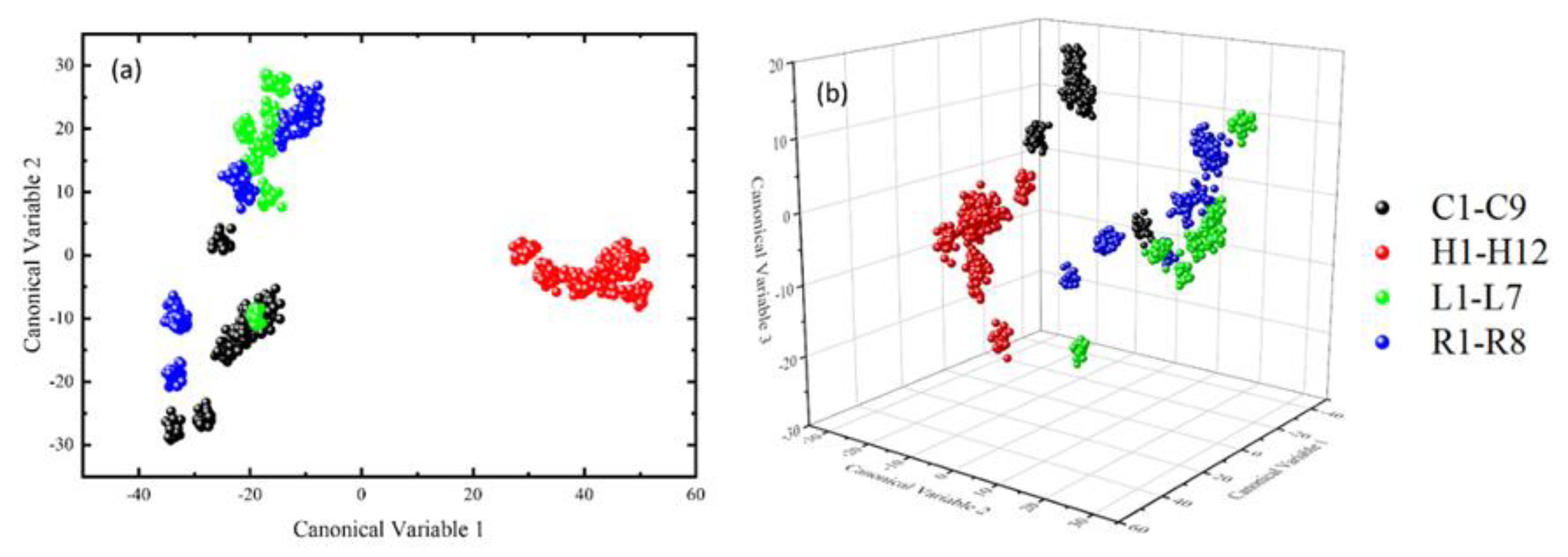
3.1. Classification Using the Raw LIBS Spectroscopic Data

At first, the raw LIBS spectroscopic data were used as inputs for the k-NN, SVC and LDA algorithmic training. The obtained accuracies were determined to be:(57.2 ± 2.7)%, (89.4 ± 0.9)% and (71.5 ± 2.4)% respectively. This finding suggests that the predictive model resulting from the k-NN algorithmic training seems to be the least successful for classification purposes in this case. In contrast, the quite high accuracy of the SVC algorithm, along with its very low standard deviation, suggests a very successful predictive model choice.

For the training of the LDA algorithm, 35 canonical variables were used (which is the maximum number of canonical variables that can be used for training, as their maximum number can be as high as the number of samples, i.e., 36 reduced by 1). As can be seen from the corresponding 2D and 3D scatter plots of Figure 2a,b, the samples H1–H12 and the C1–C9 ones were clearly distinguishable and well separated from the other samples, while some limited overlapping was found to occur for the L1–L7 and R1–R8 samples. Although the LDA algorithm provided relatively good separation between samples based on the results of these figures, its accuracy was found to be only slightly higher than 70%, making the LDA predictive model not a preferred choice. The reason for this relatively low accuracy of the LDA model is because in each cluster there exist many different samples and there is a possible extra overlapping between them, that cannot be observed visually in the plots of Figure 2a,b, due to the coloring of the clusters. Because of this situation, and in order to better evaluate the above findings, the corresponding classification reports were constructed and are shown in Table 1. The classification report offers a more detailed picture of the classification procedure, including all the samples, alongside with their behavior during the algorithmic training.

The f1-score shown in Table 1 is a weighted harmonic mean of the precision and recall parameters, so that the best score corresponds to 1.0, while the worst one corresponds to 0.0 [33]. The precision parameter denotes the ability of a classifier not to label an instance positive that is actually negative. For each class, it is defined as the ratio of true positives to the sum of true and false positives. The recall parameter expresses the ability of a classifier to find all positive instances. For each class it is defined as the ratio of true positives to the sum of true positives and false negatives. The individual values of the precision and recall parameters are not included in Table 1 for simplicity reasons, since the f1-score contains information related to both of them. The other parameter used for the evaluation of the results of Table 1, is the so-called support parameter. The support is the number of actual occurrences of a class in the specified dataset. For further evaluation of the classifier’s overall f1-score, the simple arithmetic mean of the per-class f1-scores is also used, which is called macro average. The classification report tables with precision and recall values for k-NN, SVC and LDA on raw data are presented in Tables S2a, S3a and S4a, respectively, in the Supplementary Material section.

As can been seen in Table 1, in the case of k-NN, 16 of 36 samples present f1-scores lower than 0.5, suggesting the reduced suitability of this model to classify the samples correctly. On the other hand, the macro average of 0.6 or 60% is very close to the accuracy of the algorithm which was found to be (57.2 ± 2.7)%. In contrast, all 36 samples for the case of SVC algorithm, except one, have f1-scores quite high and this can be confirmed by the average as well, which attains a value of 0.9, which is very close to the obtained algorithmic accuracy of (89.4 ± 0.9)%. These findings are important evidence that the SVC is a very robust and well-trained predictive model, able to discriminate the samples successfully and with quite high accuracy. On the contrary, the LDA algorithm was observed to exhibit difficulties in prediction, mostly from the samples C1–C9 and L1–L7, the former having 4 out of 9 samples and the latter having 4 out of 7 samples with f1-scores lower than 0.5. Interestingly, in the case of the H1–H12 and R1–R8 samples, the LDA algorithm was found operating much more successfully, yielding high f1-scores for 9 out of 12 H-samples and for 6 out of 8 R-samples.

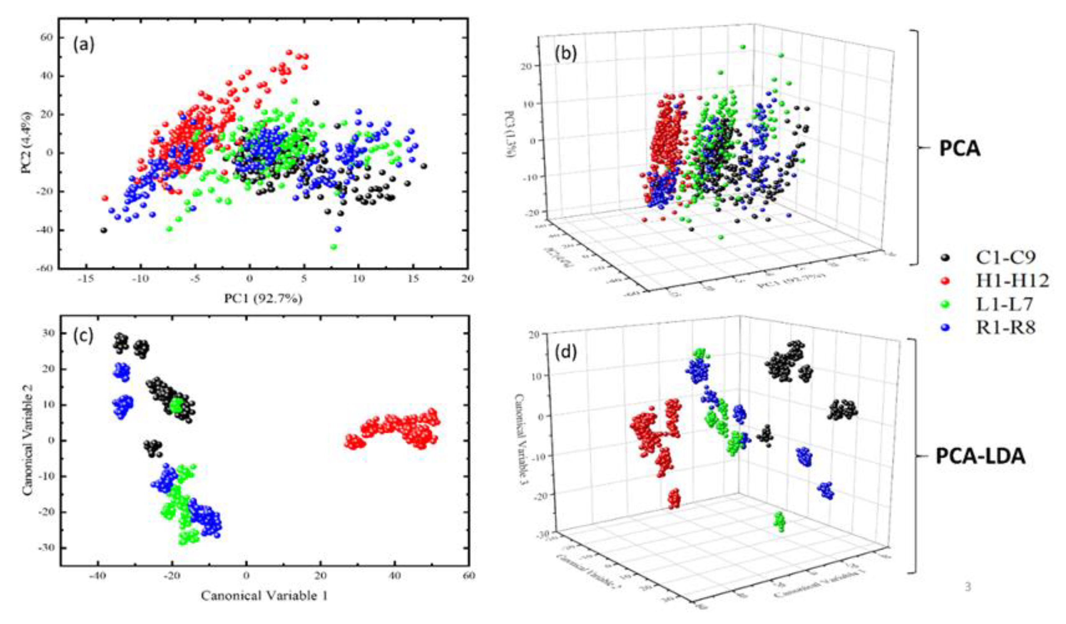
3.2. Classification Results Using the PCA Pre-Processed LIBS Spectroscopic Data

At first, the unsupervised PCA technique was employed to obtain some reduction of the dimensionality of the LIBS data, and also to search for the occurrence of any pattern, in order to proceed, in the next stage, to further classification by means of algorithmic training. The 2D and 3D score plots for the first two and three PCs are presented in Figure 3a,b respectively. As can be seen from these plots, the H-samples are clearly separated from the C-, L- and R-ones, the latter forming a separate second cluster, suffering however, from some relatively important overlapping. Nevertheless, the explained variance from the first 3 PCs were determined to be 92.7% for PC1, 4.4% for PC2 and 1.3% for PC3 with a cumulative explained ratio of the order of 98.4%. The cumulative explained variance as a function of the number of PCs considered is shown in Figure 4a. As can be seen from this plot, the use of only few principal components (PCs) seems to be quite successful as the cumulative obtained variance very quickly attains a plateau, suggesting that the use of more PCs is not as necessary, as might be expected initially.

The loadings plot for the first three PCs (i.e., PC1, PC2, PC3) are presented in Figure 4. Loadings are very important because their values relate the significance of every spectral feature from the original data with the related PC. For instance, by inspecting the plot for PC1 in Figure 4b, which has an explained variance of 92.7%, it becomes obvious that the whole spectra along with the strong background is very important in order to extract most of the variance which is explained by the first principal component, PC1. Furthermore, it seems that the CN band is more dominant than the other spectral features, while the hydrogen’s H_α and H_β spectral lines and the oxygen line have the most significant contributions for PC1. For the second principal component, PC2 (see e.g., Figure 4c), which has an explained variance of 4.4%, the previously mentioned emissions continue to contribute, with the contribution of the background being practically negligible, and thus almost vanished. The same pattern was found for the third principal component, PC3 (see e.g., Figure 4d), with an explained variance of only 1.3%. However, in this case, the C₂ bands seem to be the important features for this principal component.

Next, for the classification of the olive oils, the original dataset was pretreated through PCA and the obtained PCs were used as inputs for the k-NN, SVC and LDA algorithms. For the training of the algorithms 30 PCs were used, as Figure 4a suggests, since the 30 PCs explain more than 99% of the original variance. The accuracies of the predictive models were then found to be: (56.9 ± 2.5)%, (88.9 ± 1.2)% and (94.0 ± 1.1)% for k-NN, SVC and LDA respectively. More specifically, the classification model resulting from the k-NN algorithmic training, indicates that this algorithm is the least suitable for the classification of the present samples. In contrast, the quite high accuracies obtained, along with the extremely low standard deviations of the SVC and LDA algorithms, indicate that they are both very successful predictive models. It is interesting to mention, that the accuracies of k-NN and SVC obtained after preprocessing of the raw data, are almost the same as the accuracies achieved directly using the raw data. This observation is very important, since it suggests that dimensionality reduction does not affect the accuracy of the predictive models while in the case of the LDA, the achieved accuracy was improved by more than 20%. The scatter plots of the 2D and 3D LDA algorithm are presented in Figure 3c,d, respectively. For the training of the LDA algorithm 35 canonical variables were used. As it is shown from the scatter plots, the H-samples and all the C-samples are well distinguished from the rest of the samples, but an overlapping between the L- and R-samples is still noticeable.

To provide more insight on the k-NN, SVC and LDA algorithms’ behavior when combined with the preprocessing of the input data by PCA, the corresponding classification report was prepared and is presented as Table 2. The precision and recall values for k-NN, SVC and LDA algorithms on the preprocessed data with the PCA, are presented in the classification reports in Tables S2b, S3b and S4b, respectively, in the Supplementary Material section.

As can been seen in Table 2, in the case of k-NN, 16 of the 36 olive oil samples present f1-scores lower than 0.5, indicating that the k-NN model is not a successful choice to provide a correct classification of the present samples based on the LIBS spectroscopic data input. The macro average was found to be 0.6 or 60%, which is very close to the accuracy of the algorithm which was (56.9 ± 2.5)%. In contrast, all 36 samples in the case of the SVC algorithm (except one sample) and the LDA algorithm, have quite high f1-scores, a finding which is further confirmed by the averages, which attained values of 0.9 and 1.0 respectively. It should be mentioned that the values of the averages are very similar to the obtained algorithmic accuracies, which were (88.9 ± 1.2)% and (94.0 ± 1.1)% respectively. Therefore, it results, that in the case of the LIBS data preprocessed by PCA, both the SVC and especially the LDA predictive models were found to exhibit very high accuracies and great robustness.

It must be emphasized at this point, that during the hyperparameter tuning of the SVC algorithm, the optimum kernel that was chosen for training was a linear one. Considering that both, LDA and PCA, are linear transformation techniques (in contrast to the k-NN which is a non-linear model), it is obvious that the LIBS spectroscopic data that were used are most probably better characterized by linear correlations and for this reason linear models are found to be more effective for their treatment and discrimination purposes. Summarizing the accuracies determined for the different predictive models employed were determined as follows: for the non-preprocessed LIBS data: k-NN: (57.2 ± 2.7)%, SVC: (89.4 ± 0.9)%, LDA: (71.5 ± 2.4)% and for the PCA preprocessed LIBS data: k-NN: (56.9 ± 2.5)%, SVC: (88.9 ± 1.2)%, LDA: (94.0 ± 1.1)%.

To further validate the accuracy of the obtained results, an external validation procedure was also performed, by utilizing the most successful model created in this work, i.e., LDA with PCA pre-processing. In that way the predictive abilities of our models can be further tested. In this case, the training set contained 25 LIBS spectra from each oil sample (i.e., samples C1–C9, H1–H12, L1–L7 and R1–R8), while the test set contained 5 unique LIBS spectra from each sample, as well. The training was performed with 5-fold cross-validation and attained a predictive accuracy of (94.1 ± 1.6)%, by using 30 PCs as inputs. The prediction accuracy by using the created model to validate the test set reached 93.88% agreement with the training data. These results are summarized in Table 3.

To the best of our knowledge, there are only two studies reported in the literature employing LIBS assisted by machine learning approaches, aiming to discriminate/classify olive oils in terms of their geographical origins. In the first of them, reference [13], neural networks have been used to provide a successful classification of the studied oils, attaining an accuracy of 95%. However, the samples employed were typical commercial edible oils (from the local market), containing different brands and grades (e.g., olive oil, sunflower and hazelnut and corn oils). In addition, these oils were produced in four different countries (i.e., Spain, Italy, Greece, and Argentina) with very different climatic and soil conditions. Most importantly, only some of the studied oils were of extra virgin olive quality. All these factors can increase the differences between the samples, this situation being reflected on the corresponding LIBS spectra; therefore, facilitating their classification. In other words, the differences of the LIBS spectra could be sizeable thus allowing for a more efficient discrimination/classification. To avoid exposure on such ambiguities, special care has been taken in the present study to employ only well characterized olive oils of extra virgin quality.

In the second study [15], different machine learning techniques (e.g., LDA, SVC and RFCs (Random Forest Classifiers)) were used for the classification of some extra virgin olive oils collected directly from the producers based on their acidity and geographical origin. Although it was a preliminary study, the reported results were very successful.

In order to further validate and better explore the capabilities of LIBS assisted by machine learning a much larger number of olive oil samples were collected and became available within the framework of a national project aiming to study and characterize the Greek olive oils. These constitute a first reliable data set, with olive oil samples being characterized by several research groups working in different scientific fields (e.g., agronomy, chemistry, biology, microbiology, etc.) all related to olive trees and olive oil research. In that view, this first attempt, employing a reliable and homogenized set of samples, all of them of extra virgin quality, is of great importance in order to evaluate the capacity of the LIBS technique and to assess the suitability and the robustness of the machine learning algorithmic approaches which were chosen to assist LIBS in terms of classification and authentication issues of olive oils.

From the above first very encouraging results, it becomes evident that the implementation of the machine learning algorithms can greatly assist the LIBS technique to achieve successful discrimination between olive oils originating from different geographical areas. The application of k-NN and SVC algorithms combined with the pretreatment of the LIBS spectroscopic data with the PCA algorithm makes possible the improvement of the results and the extraction of valuable information from the LIBS spectra which otherwise would not have been identified.

4. Conclusions

In the present work, the LIBS technique combined with some of the most popular, open source, machine learning algorithms were used with great success for the discrimination/classification of some olive oils in terms of their geographical origin. Classification accuracies exceeding 90% were attained, suggesting the potential of this approach. In addition to the discrimination/classification issues, the effect of pre-processing of the LIBS spectroscopic data on the accuracy of the different predictive models was also investigated. It was found that pre-processing of the LIBS spectroscopic data, e.g., with the PCA algorithm, can improve the accuracy of some predictive models, e.g., the LDA one, while leaving unaffected the classification accuracies of k-NN and SVC models, despite the dimensionality reduction achieved. In fact, the pre-processing of the LIBS spectroscopic data with PCA has a great impact on the LDA predictive model accuracy, this last attaining a value up to (94.0 ± 1.1)%. Overall, it can be concluded that pre-processing of the LIBS spectroscopic data by the PCA algorithm can be an effective method for minimization of the training time while, in some cases, it can considerably enhance the obtained accuracies.

In addition, it was found that the most suitable and efficient machine learning models, in the case of such LIBS spectroscopic data sets, seem to be the linear ones. This qualitative finding is of great importance, because the selection of a suitable predictive model is not an easy task while, in general, there is no “rule of thumb”, indicating what kind of algorithms are best suited for a specific task. Concluding, based on the great results obtained so far from LIBS measurements, and for a relatively small geographical region, i.e., the island of Crete, it can be expected that the next step, would be the validation of the presented approach on a larger geographical scale, which would include more regions and even more countries.

References

1. European Union. Regulation (EU) No 1151/2012 of the European Parliament and of the Council of 21 November 2012 on quality schemes for agricultural products and foodstuffs. Off. J. Eur. Union 2012, L343, 1–29. [Google Scholar]
2. Boskou, D. Olive Oil: Chemistry and Technology, 2nd ed.; AOCS Publishing: Champaign, IL, USA, 2006. [Google Scholar]
3. Likudis, Z. Olive Oils with Protected Designation of Origin (PDO) and Protected Geographical Indication (PGI). In Products from Olive Tree; Boskou, D., Clodoveo, M.L., Eds.; IntechOpen: London, UK, 2016. [Google Scholar] [CrossRef] [Green Version]
4. Markiewicz-Keszycka, M.; Cama-Moncunill, R.; Casado-Gavalda, M.P.; Sullivan, C.; Cullen, P.J. Laser-induced breakdown spectroscopy for food authentication. Curr. Opin. Food Sci. 2019, 28, 96–103. [Google Scholar] [CrossRef]
5. Standards and Methods. Available online: http://www.internationaloliveoil.org/estaticos/view/224-testing-methods (accessed on 18 December 2019).
6. Longobardi, F.; Ventrella, A.; Napoli, C.; Humpfer, E.; Schütz, B.; Schäfer, H.; Kontominas, M.G.; Sacco, A. Classification of olive oils according to geographical origin by using 1H NMR fingerprinting combined with multivariate analysis. Food Chem. 2012, 130, 177–183. [Google Scholar] [CrossRef]
7. Petrakis, P.V.; Agiomyrgianaki, A.; Christophoridou, S.; Spyros, A.; Dais, P. Geographical Characterization of Greek Virgin Olive Oils (Cv. Koroneiki) Using1H and31P NMR Fingerprinting with Canonical Discriminant Analysis and Classification Binary Trees. J. Agric. Food Chem. 2008, 56, 3200–3207. [Google Scholar] [CrossRef]
8. Tapp, H.S.; Defernez, M.; Kemsley, E.K. FTIR Spectroscopy and Multivariate Analysis Can Distinguish the Geographic Origin of Extra Virgin Olive Oils. J. Agric. Food Chem. 2003, 51, 6110–6115. [Google Scholar] [CrossRef]
9. Bendini, A.; Cerretani, L.; Di Virgilio, F.; Belloni, P.; Bonoli-Carbognim, M.; Lercker, G. Preliminary Evaluation of the Application of the FTIR Spectroscopy to Control the Geographic Origin and Quality of Virgin Olive Oils. J. Food Qual. 2007, 30, 424–437. [Google Scholar] [CrossRef]
10. Korifi, R.; Le Dréau, Y.; Molinet, J.; Artaud, J.; Dupuy, N. Composition and authentication of virgin olive oil from French PDO regions by chemometric treatment of Raman spectra. J. Raman Spectrosc. 2011, 42, 1540–1547. [Google Scholar] [CrossRef]
11. Sánchez-López, E.; Sánchez-Rodríguez, M.I.; Marinas, A.; Marinas, J.M.; Urbano, F.J.; Caridad, J.M.; Moalem, M. Chemometric study of Andalusian extra virgin olive oils Raman spectra: Qualitative and quantitative information. Talanta 2016, 156–157, 180–190. [Google Scholar] [CrossRef]
12. Craig, A.P.; Franca, A.S.; Irudayaraj, J. Surface-Enhanced Raman Spectroscopy Applied to Food Safety. Annu. Rev. Food Sci. Technol. 2013, 4, 369–380. [Google Scholar] [CrossRef]
13. Caceres, J.O.; Moncayo, S.; Rosales, J.D.; de Villena, F.J.M.; Alvira, F.C.; Bilmes, G.M. Application of Laser-Induced Breakdown Spectroscopy (LIBS) and Neural Networks to Olive Oils Analysis. Appl. Spectrosc. 2013, 67, 1064–1072. [Google Scholar] [CrossRef]
14. Mbesse Kongbonga, Y.G.; Ghalila, H.; Onana, M.B.; Ben Lakhdar, Z. Classification of vegetable oils based on their concentration of saturated fatty acids using laser induced breakdown spectroscopy (LIBS). Food Chem. 2014, 147, 327–331. [Google Scholar] [CrossRef] [PubMed]
15. Gazeli, O.; Bellou, E.; Stefas, D.; Couris, S. Laser-based classification of olive oils assisted by machine learning. Food Chem. 2020, 302, 125329. [Google Scholar] [CrossRef] [PubMed]
16. Cremers, D.A.; Radziemski, L.J. Handbook of Laser-Induced Breakdown Spectroscopy; Wiley-Blackwell: Oxford, UK, 2013. [Google Scholar]
17. De Giacomo, A.; Hermann, J. Laser-induced plasma emission: From atomic to molecular spectra. J. Phys. D Appl. Phys. 2017, 50, 183002. [Google Scholar] [CrossRef]
18. Zhang, T.; Tang, H.; Li, H. Chemometrics in laser-induced breakdown spectroscopy. J. Chemom. 2018, 32, e2983. [Google Scholar] [CrossRef]
19. Zhang, Y.; Sun, C.; Gao, L.; Yue, Z.; Shabbir, S.; Xu, W.; Wu, M.; Yu, J. Determination of minor metal elements in steel using laser-induced breakdown spectroscopy combined with machine learning algorithms. Spectrochim. Acta Part B At. Spectrosc. 2020, 166, 105802. [Google Scholar] [CrossRef]
20. Sattmann, R.; Monch, I.; Krause, H.; Noll, R.; Couris, S.; Hatziapostolou, A.; Mavromanolakis, A.; Fotakis, C.; Larrauri, E.; Miguel, R. Laser-Induced Breakdown Spectroscopy for Polymer Identification. Appl. Spectrosc. 1998, 52, 456–461. [Google Scholar] [CrossRef]
21. Stefas, D.; Gyftokostas, N.; Bellou, E.; Couris, S. Laser-Induced Breakdown Spectroscopy Assisted by Machine Learning for Plastics/Polymers Identification. Atoms 2019, 7, 79. [Google Scholar] [CrossRef] [Green Version]
22. Singh, V.K.; Sharma, J.; Pathak, A.K.; Ghany, C.T.; Gondal, M.A. Laser-induced breakdown spectroscopy (LIBS): A novel technology for identifying microbes causing infectious diseases. Biophys. Rev. 2018, 10, 1221–1239. [Google Scholar] [CrossRef]
23. Gaudiuso, R.; Melikechi, N.; Abdel-Salam, Z.A.; Harith, M.A.; Palleschi, V.; Motto-Ros, V.; Busser, B. Laser-induced breakdown spectroscopy for human and animal health: A review. Spectrochim. Acta Part B At. Spectrosc. 2019, 152, 123–148. [Google Scholar] [CrossRef]
24. Liu, F.; Ye, L.; Peng, J.; Song, K.; Shen, T.; Zhang, T.; He, Y. Fast Detection of copper content in rice by laser-induced breakdown spectroscopy with uni- and multivariate analysis. Sensors 2018, 18, 705. [Google Scholar] [CrossRef] [Green Version]
25. Chen, C.-T.; Banaru, D.; Sarnet, T.; Hermann, J. Two-step procedure for trace element analysis in food via calibration-free laser-induced breakdown spectroscopy. Spectrochim. Acta Part B At. Spectrosc. 2018, 150, 77–85. [Google Scholar] [CrossRef] [Green Version]
26. Zivkovic, S.; Savovic, J.; Kuzmanovic, M.; Petrovic, J.; Momcilovic, M. Alternative analytical method for direct determination of Mn and Ba in peppermint tea based on laser induced breakdown spectroscopy. Microchem. J. 2018, 137, 410–417. [Google Scholar] [CrossRef]
27. European Union Commission. Commission Delegated Regulation No 2016/2095 of 26 September 2016 amending Regulation (EEC) No 2568/91 on the characteristics of olive oil and olive-residue oil and on the relevant methods of analysis. Off. J. Eur. Union 2016, L326, 1–6. [Google Scholar]
28. Pedregosa, F.; Varoquaux, G.; Gramfort, A.; Michel, V.; Thirion, B.; Grisel, O.; Blondel, M.; Prettenhofer, P.; Weiss, R.; Dubourg, V.; et al. Scikit-learn: Machine Learning in Python. J. Mach. Learn. Res. 2011, 12, 2825–2830. [Google Scholar]
29. Jolliffe, I.T. Principal Component Analysis; Springer: New York, NY, USA, 2011. [Google Scholar]
30. Tharwat, A.; Gaber, T.; Ibrahim, A.; Hassanien, A.E. Linear discriminant analysis: A detailed tutorial. AIC 2017, 30, 169–190. [Google Scholar] [CrossRef] [Green Version]
31. Cover, T.; Hart, P. Nearest neighbor pattern classification. IEEE Trans. Inf. Theory 1967, 13, 21–27. [Google Scholar] [CrossRef]
32. Cortes, C.; Vapnik, V. Support-vector networks. Mach. Learn. 1995, 20, 273–297. [Google Scholar] [CrossRef]
33. Powers, D.M.W. Evaluation: From Precision, Recall and F-Factor to ROC, Informedness, Markedness & Correlation; Technical Report SIE-07-001; School of Informatics and Engineering, Flinders University: Adelaide, Australia, 2007. [Google Scholar]
Figure 1. (a) Geographical distribution of the studied olive oils, (b) LIBS spectra of 4 representative samples, i.e., samples C1, H1, L1 and R1.
Applsci 10 03462 g001
Figure 2. (a) 2D and (b) 3D LDA scatter plots corresponding to the olive oil samples from Chania (C), Heraklion (H), Lasithi (L) and Rethymnon (R) regions.
Applsci 10 03462 g002
Figure 3. PCA (a) 2D and (b) 3D score plots and PCA-LDA (c) 2D and (d) 3D scatter plots corresponding to the olive oil samples from Chania (C), Herakleion (H), Lasithi (L) and Rethymnon (R) regions.
Applsci 10 03462 g003
Figure 4. (a) Cumulative explained variance, loadings plots for (b) PC1, (c) PC2, and (d) PC3.
Applsci 10 03462 g004