Similarity Analysis for Time Series-Based 2D Temperature Measurement of Engine Exhaust Gas in TDLAT

Abstract
1. Introduction
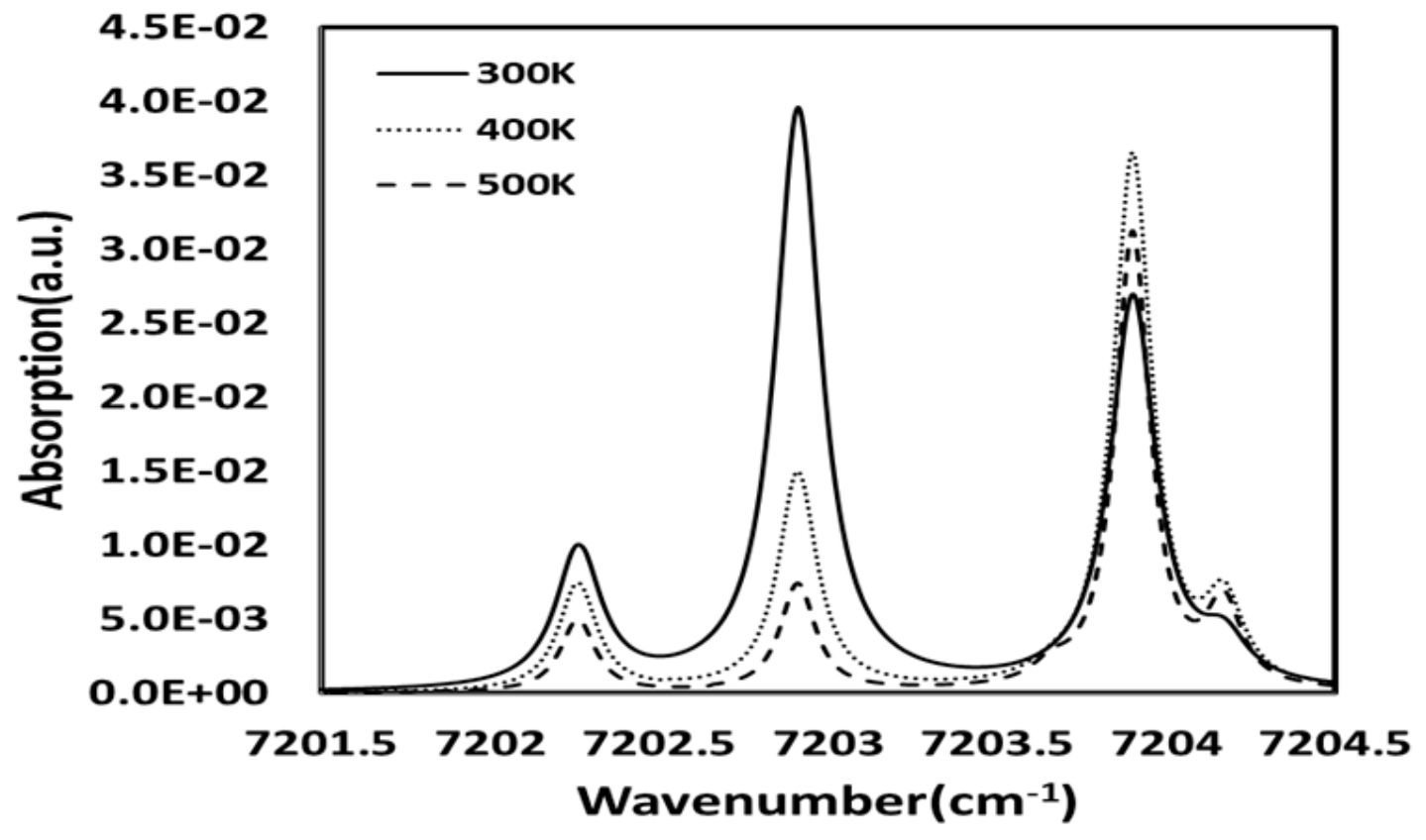
2. Theory of TDLAS
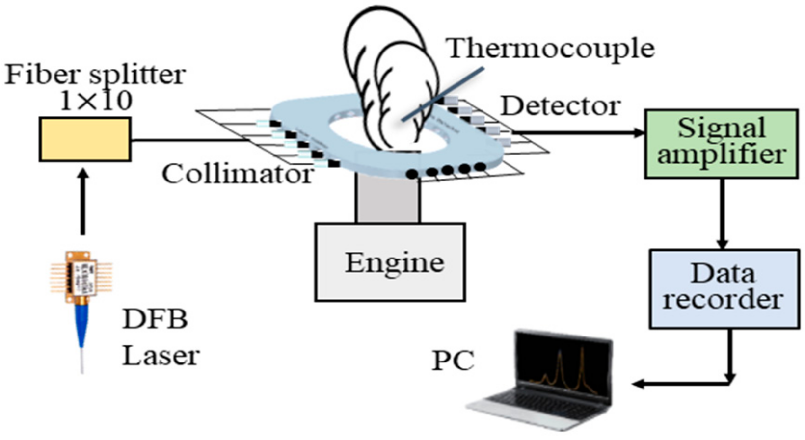
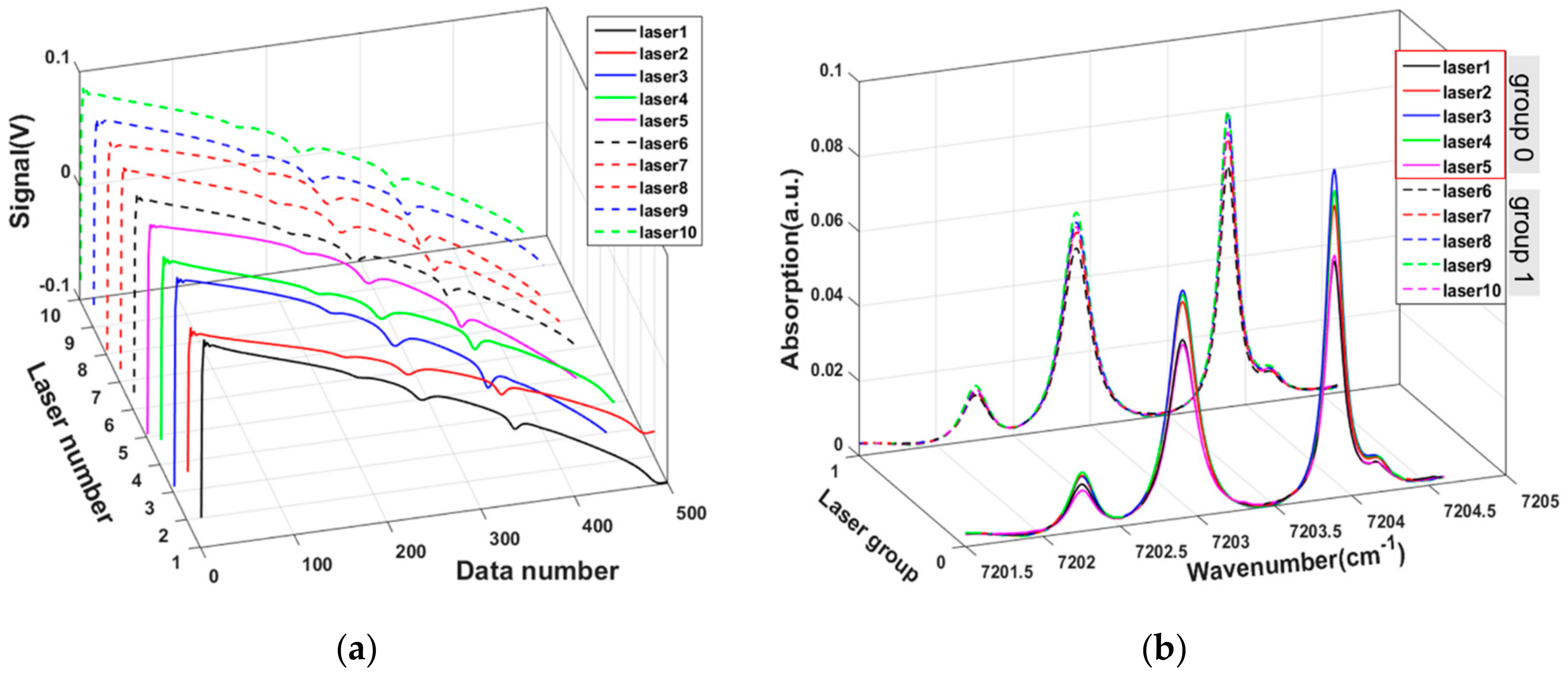
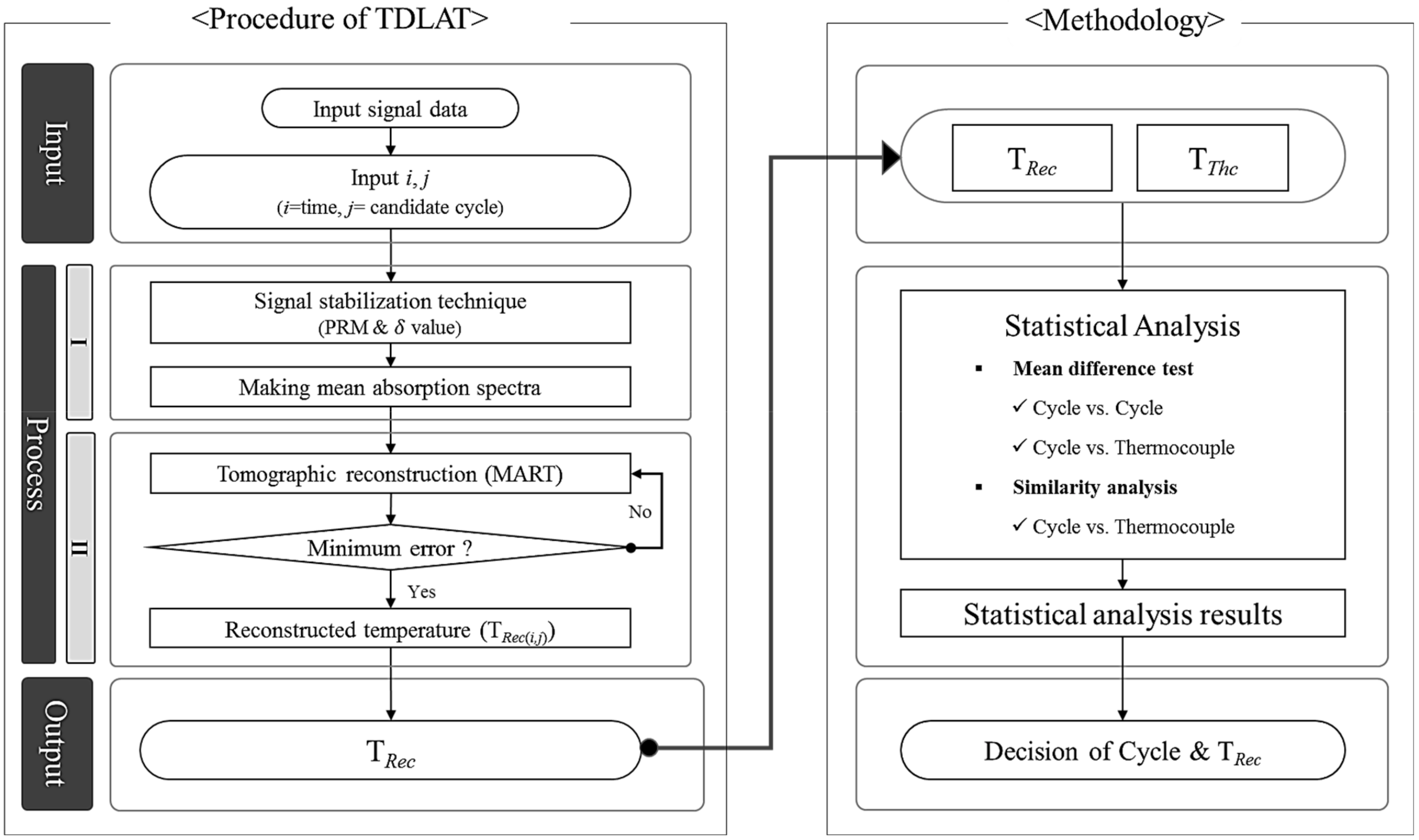
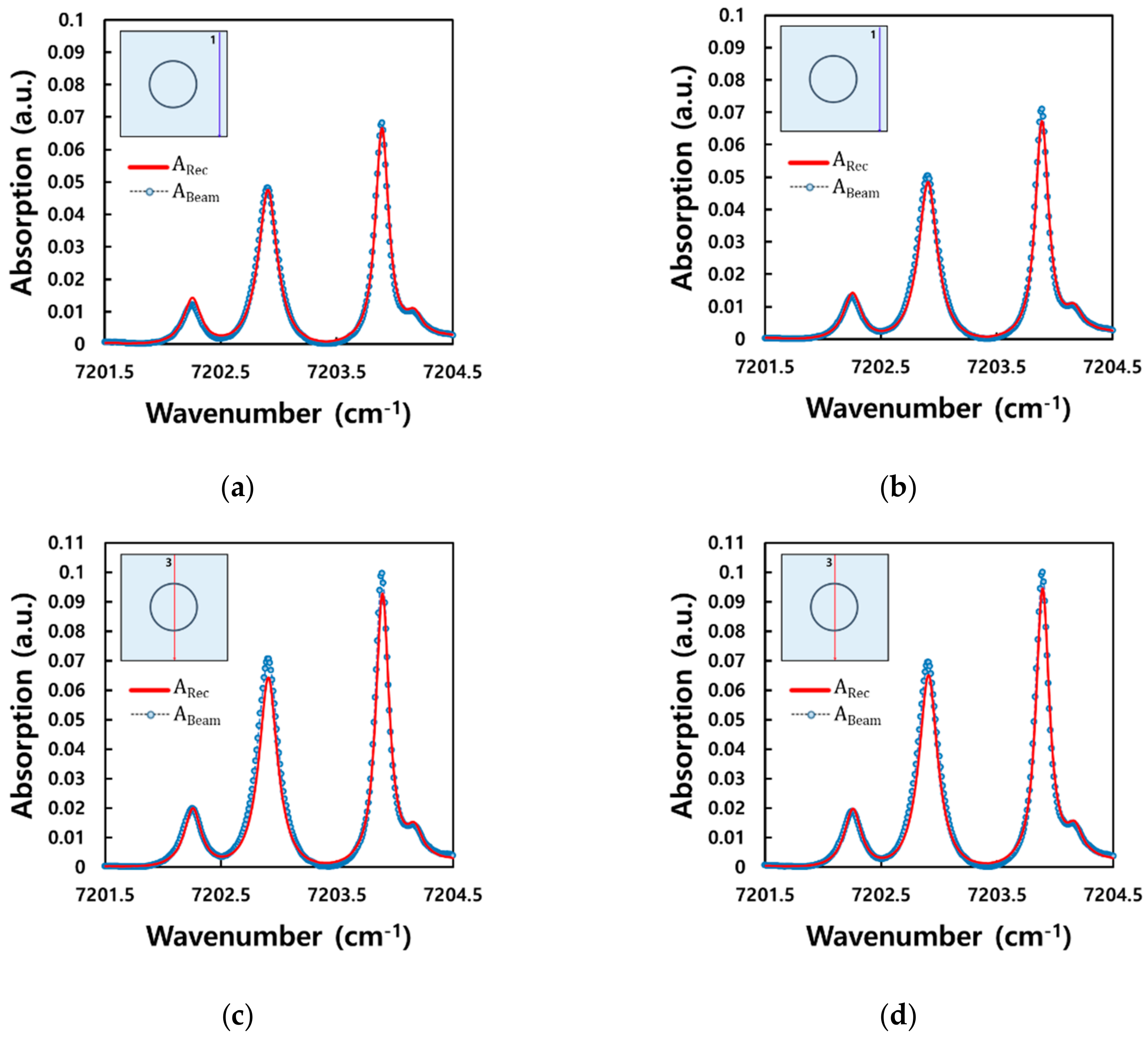
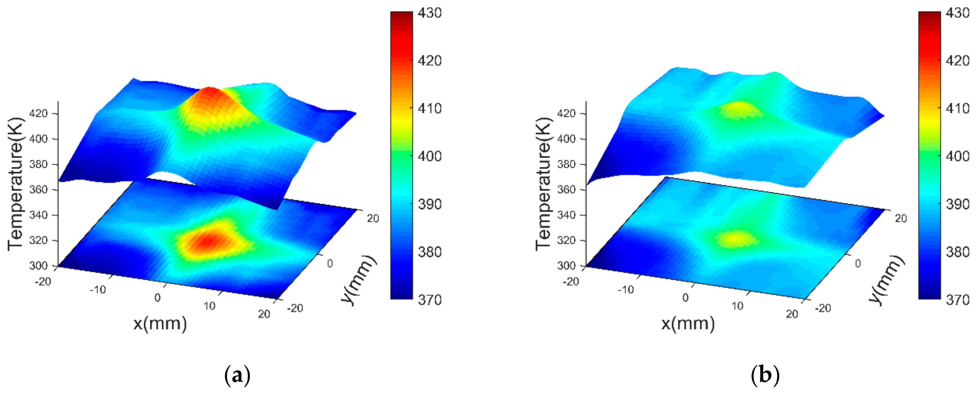
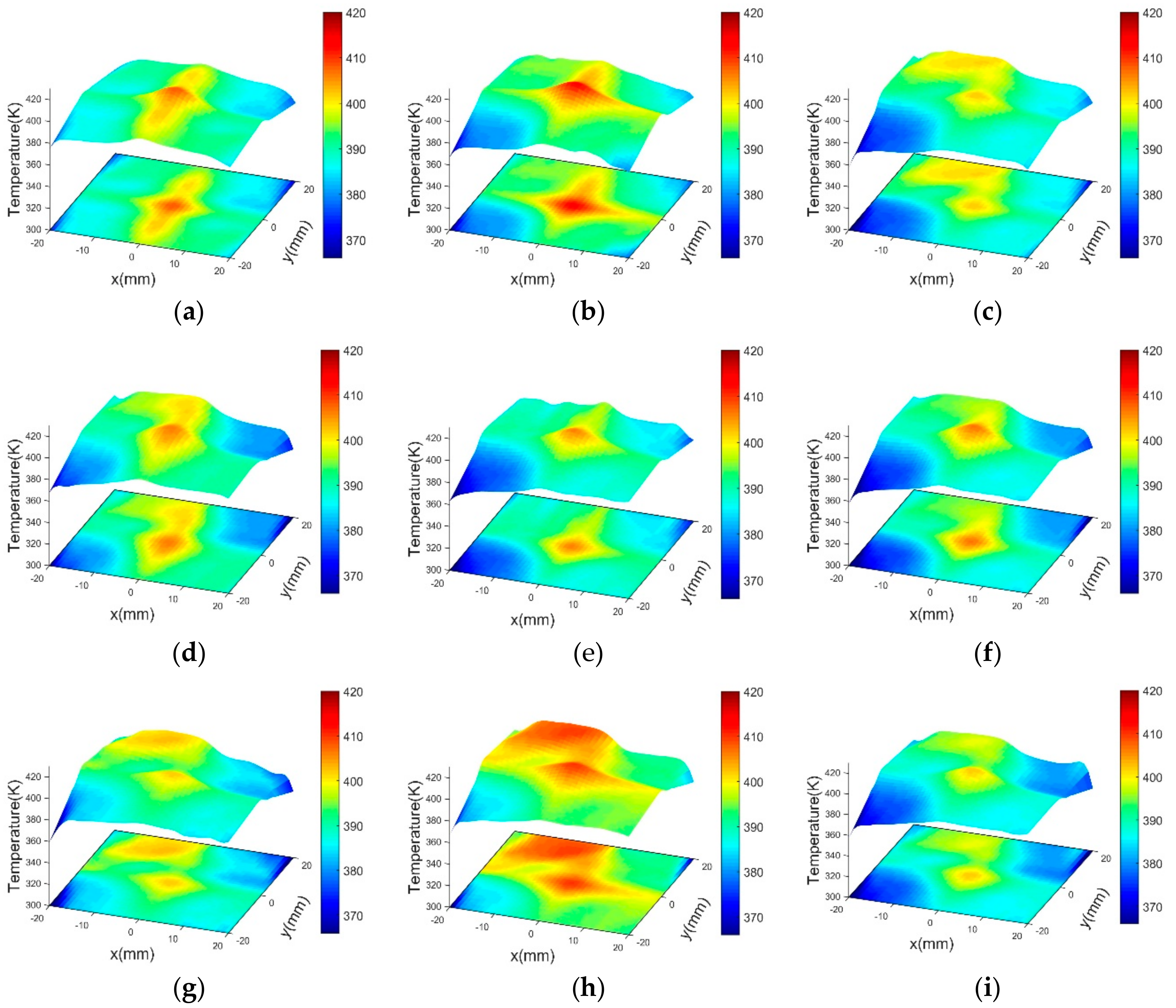
3. Experiment and Tomography Analysis
4. Statistical-Based Mean Difference Test and Similarity Analysis
4.1. [Step 1] Mean Difference Test
4.1.1. Paired t Test
- Null hypothesis: (the population mean of the difference () equals the hypothesized mean of the difference ().
- Alternative hypothesis: (the population mean of the difference () does not equal the hypothesized mean of the difference ().
4.1.2. Results of Mean Difference Test in [Step 1]
4.2. [Step 2] Similarity Analysis
4.2.1. Two-Sample t-Test
- Null hypothesis: H0: = Thcg Recg = (the difference between the population means (Thcg Recg) is equal to the hypothesized difference ()).
- Alternative hypothesis: H1: = Thcg Recg (the difference between the population means (Thcg Recg) is not equal to the hypothesized difference ()).
4.2.2. Root Mean Square Error (RMSE)
4.2.3. Time-Based Mahalanobis Distance (TMD)
4.2.4. Results of Similarity Analysis in [Step 2]
5. Conclusions
Author Contributions
Funding
Conflicts of Interest
Appendix A

| Cycles | Time (s) | |||||||||
|---|---|---|---|---|---|---|---|---|---|---|
| 1 | 2 | 3 | 4 | 5 | 6 | 7 | 8 | 9 | ||
| P-Value | ||||||||||
| 31 | <0.05 | 0.055 | <0.05 | <0.05 | 0.094 | <0.05 | <0.05 | <0.05 | <0.05 | |
| 51 | <0.05 | <0.05 | 0.175 | <0.05 | 0.062 | 0.105 | <0.05 | <0.05 | 0.205 | |
| 71 | <0.05 | <0.05 | 0.127 | <0.05 | 0.117 | <0.05 | <0.05 | <0.05 | 0.071 | |
| 91 | 0.071 | <0.05 | 0.109 | <0.05 | 0.265 | 0.073 | 0.071 | <0.05 | 0.099 | |
| 111 | 0.160 | 0.053 | 0.142 | <0.05 | 0.426 | 0.162 | 0.392 | 0.060 | 0.207 | |
| 151 | 0.099 | 0.213 | 0.218 | <0.05 | 0.401 | 0.706 | 0.106 | <0.05 | 0.143 | |
| 201 | 0.581 | 0.215 | 0.152 | 0.168 | 0.997 | 0.617 | 0.104 | <0.05 | 0.832 | |
| 251 | 0.899 | 0.148 | 0.115 | 0.280 | 0.645 | 0.688 | 0.388 | 0.302 | 0.678 | |
| 301 | 0.349 | 0.276 | 0.066 | 0.355 | 0.466 | 0.173 | 0.801 | 0.635 | 0.537 | |
| 351 | 0.398 | 0.285 | 0.220 | 0.181 | 0.614 | 0.271 | 0.660 | 0.758 | 0.391 | |
| 401 | <0.05 | 0.248 | 0.153 | 0.358 | 0.499 | <0.05 | 0.529 | 0.565 | 0.062 | |
| 451 | 0.054 | 0.243 | 0.284 | 0.227 | 0.348 | 0.064 | 0.358 | 0.867 | 0.125 | |
| 501 | <0.05 | 0.427 | 0.379 | 0.562 | 0.332 | <0.05 | 0.114 | 0.127 | <0.05 | |
| 601 | <0.05 | 0.548 | 0.794 | 0.854 | 0.387 | <0.05 | <0.05 | <0.05 | <0.05 | |
| 701 | <0.05 | 0.247 | 0.832 | 0.833 | 0.281 | <0.05 | <0.05 | <0.05 | <0.05 | |
| 801 | <0.05 | 0.413 | 0.607 | 0.565 | 0.231 | <0.05 | <0.05 | <0.05 | <0.05 | |
| 901 | <0.05 | 0.352 | 0.729 | 0.441 | 0.210 | <0.05 | <0.05 | <0.05 | <0.05 | |
| 1001 | <0.05 | 0.687 | 0.343 | 0.383 | 0.103 | <0.05 | <0.05 | <0.05 | <0.05 | |
References
- Amin, R.; Galen, B.F.; John, W.H.; Joseph, R.T.; James, D.P.; Christine, K.L. Rapidly pulsed reductants for diesel NOx reduction with lean NOx traps: Effects of pulsing parameters on performance. Appl. Catal. B Environ. 2018, 223, 177–191. [Google Scholar]
- Perng, C.C.; Easterling, V.G.; Harold, M.P. Fast lean-rich cycling for enhanced NOx conversion on storage and reduction catalysts. Catal. Today 2014, 231, 125–134. [Google Scholar] [CrossRef]
- Lietti, L.; Artioli, N.; Righini, L.; Castoldi, L.; Forzatti, P. Pathways for N2 and N2O formation during the reduction of NOx over Pt–Ba/Al2O3 LNT catalysts investigated by labeling isotopic experiments. Ind. Eng. Chem. Res. 2012, 51, 7597–7605. [Google Scholar] [CrossRef]
- Roy, S.; Gord, J.R.; Patnaik, A.K. Recent advances incoherent anti-Stokes Raman scattering spectroscopy: Fundamental developments and applications in reacting flows. Prog. Energy Combust. Sci. 2010, 36, 280–306. [Google Scholar] [CrossRef]
- Steuwe, C.; Kaminski, C.F.; Baumberg, J.J.; Mahajan, S. Surface enhanced coherent anti-Stokes Raman scattering on nanostructured gold surfaces. Nano Lett. 2011, 11, 5339–5343. [Google Scholar] [CrossRef] [PubMed]
- Williams, B.; Edwards, M.; Stone, R.; Williams, J.; Ewart, P. High precision in-cylinder gas thermometry using laser induced gratings: Quantitative measurement of evaporative cooling with gasoline/alcohol blends in a GDI optical engine. Combust. Flame 2014, 161, 270–279. [Google Scholar] [CrossRef]
- Hoffman, D.; Münch, K.U.; Leipertz, A. Two-dimensional temperature determination in sooting flames by filtered Rayleigh scattering. Opt. Lett. 1996, 21, 525–527. [Google Scholar] [CrossRef]
- Itani, L.; Bruneaux, G.; Lella, A.; Schulz, C. Two-tracer LIF imaging of preferential evaporation of multi-component gasoline fuel sprays under engine conditions. Proc. Combust. Inst. 2015, 35, 2915–2922. [Google Scholar] [CrossRef]
- Cho, K.Y.; Satija, A.; Pourpoint, T.L.; Son, S.F.; Lucht, R.P. High-repetition-rate three-dimensional OH imaging using scanned planar laser-induced fluorescence system for multiphase combustion. Appl. Opt. 2014, 53, 316–326. [Google Scholar] [CrossRef]
- Deguchi, Y.; Yasui, D.; Adachi, A. Development of 2D temperature and concentration measurement method using tunable diode laser absorption spectroscopy. J. Mech. Eng. Autom. 2012, 2, 543–549. [Google Scholar]
- Ma, L.; Li, X.; Sanders, S.T.; Caswell, A.W.; Roy, S.; Plemmons, D.H.; Gord, J.R. 50-kHz-rate 2D imaging of temperature and H2O concentration at the exhaust plane of a J85 engine using hyperspectral tomography. Opt. Express 2013, 21, 1152–1162. [Google Scholar] [CrossRef] [PubMed]
- Busa, K.M.; Ellison, E.N.; McGovern, B.J.; McDaniel, J.C.; Diskin, G.S.; DePiro, M.J.; Capriotti, D.P.; Gaffney, R.L. Measurements on NASA Langley Durable Combustor Rig by TDLAT: Preliminary Results. In Proceedings of the 51st AIAA Aerospace Sciences Meeting Including New Horizons Forum and Aerospace Exposition, Grapevine, TX, USA, 7–10 January 2013. [Google Scholar]
- Busa, K.M.; Rice, B.E.; McDaniel, J.C.; Goyne, C.P.; Rockwell, R.D.; Fulton, J.A.; Edwards, J.R.; Diskin, G.S. Scramjet combustion efficiency measurement via tomographic absorption spectroscopy and particle image velocimetry. AIAA J. 2016, 54, 2463–2471. [Google Scholar] [CrossRef]
- Sun, P.; Zhang, Z.; Li, Z.; Gou, Q.; Dong, F. Study of two dimensional tomography reconstruction of temperature and gas concentration in combustion field using TDLAS. Appl. Sci. 2017, 7, 990. [Google Scholar] [CrossRef]
- Zhang, Z.R.; Pang, T.; Yang, Y.; Xia, H.; Cui, X.; Sun, P.; Wu, B.; Wang, Y.; Sigrist, M.W.; Dong, F. Development of a tunable diode laser absorption sensor for online monitoring of industrial gas total emissions based on optical scintillation cross-correlation technique. Opt. Express 2016, 24, 943–955. [Google Scholar] [CrossRef] [PubMed]
- Dickheuer, S.; Marchuk, O.; Tsankov, T.V.; Luggenhölscher, D.; Czarnetzki, W.; Ertmer, S.; Kreter, A. Measurement of the magnetic field in a linear magnetized plasma by tunable diode laser absorption spectroscopy. Atoms 2019, 7, 48. [Google Scholar] [CrossRef]
- Stritzke, F.; Kely, S.V.D.; Feiling, A.; Dreizler, A.; Wagner, S. TDLAS-based NH3 mole fraction measurement for exhaust diagnostics during selective catalytic reduction using a fiber-coupled 2.2-µm DFB diode laser. Opt. Express 2015, 119, 143–152. [Google Scholar] [CrossRef]
- Bolshov, M.A.; Kuritsyn, Y.A.; Romanovskii, Y.V. Tunable diode laser spectroscopy as a technique for combustion diagnostics. Spectrochim. Acta Part B 2015, 106, 45–66. [Google Scholar] [CrossRef]
- Xu, L.; Liu, C.; Jing, W.; Cao, Z.; Xue, X.; Lin, Y. Tunable diode laser absorption spectroscopy-based tomography system for on-line monitoring of two-dimensional distributions of temperature and H2O mole fraction. Rev. Sci. Instrum. 2016, 87, 013101. [Google Scholar] [CrossRef]
- Gamache, R.R.; Kennedy, S.; Hawkins, R.; Rothman, L.S. Total internal partition sums for molecules in the terrestrial atmosphere. J. Mol. Struct. 2000, 517–518, 407–425. [Google Scholar] [CrossRef]
- Rothman, L.S.; Gordon, I.E.; Barbe, A.; Benner, D.C.; Bernath, P.F.; Birk, M.; Bizzocchi, L.; Boudon, V.; Brown, L.R.; Campargue, A.; et al. The HITRAN2012 molecular spectroscopic database. J. Quant. Spectrosc. Radiat. Transf. 2013, 130, 4–50. [Google Scholar] [CrossRef]
- Hong, D.H.; Wang, L.; Truong, T.K. Low-complexity direct computation algorithm for cubic-spline interpolation scheme. J. Vis. Commun. Image Represent. 2018, 50, 159–166. [Google Scholar] [CrossRef]
- Deguchi, Y.; Noda, M.; Abe, M.; Abe, M. Improvement of combustion control through real-time measurement of O2 and CO concentrations in incinerators using diode laser absorption spectroscopy. Proc. Combust. Inst. 2002, 29, 147–153. [Google Scholar] [CrossRef]
- Choi, D.W.; Jeon, M.G.; Cho, G.R.; Kamimoto, T.; Deguchi, Y.; Doh, D.H. Performance improvements in temperature reconstructions of 2-D tunable diode laser absorption spectroscopy (TDLAS). J. Therm. Sci. 2016, 25, 84–89. [Google Scholar] [CrossRef]
- Zaatar, Y.; Bechara, J.; Khoury, A.; Zaouk, D.; Charles, J.-P. Diode laser sensor for process control and environmental monitoring. Appl. Energy 2000, 65, 107–113. [Google Scholar] [CrossRef]
- Doh, D.H.; Lee, C.J.; Cho, G.R.; Moon, K.R. Performances of Volume-PTV and Tomo-PIV. Open J. Fluid Dyn. 2012, 2, 368–374. [Google Scholar] [CrossRef]
- Choi, K.M.; Lee, J.T.; Jeon, S.G.; Hong, T.G.; Paek, J.K.; Han, S.H.; Yim, D.S. A review of fundamentals of statistical concepts in clinical trials. J. Korean Soc. Clin. Pharmacol. Ther. 2012, 20, 109–124. [Google Scholar] [CrossRef][Green Version]
- Cort, J.W.; Kenhi, M. Advantages of the mean absolute error (MAE) over the root mean square error (RMSE) in assessing average model performance. Clim. Res. 2015, 30, 79–82. [Google Scholar]
- Seo, M.K.; Yun, W.Y. Clustering based hot strip roughing mill diagnosis using Mahalanobis distance. J. Korean Inst. Ind. Eng. 2017, 43, 298–307. [Google Scholar]
- Wikipedia. Available online: https://en.wikipedia.org/wiki/Mahalanobis_distance (accessed on 23 September 2019).
- Yu, J.W.; Jang, J.Y.; Yoo, J.Y.; Kim, S.S. Fault detection method for steam boiler tube using Mahalanobis distance. J. Korean Inst. Intell. Syst. 2016, 26, 246–252. [Google Scholar] [CrossRef][Green Version]
- Minitab 19 Support. Available online: https://support.minitab.com/en-us/minitab/18/Assistant_Two_Sample_t.pdf (accessed on 20 November 2019).


| No. | Time (s) | TRec | ||||
|---|---|---|---|---|---|---|
| 31 | 51 | 901 | 1001 | |||
| 1 | 1.0 | 404.833 | 400.000 | 405.432 | 404.189 | |
| 2 | 406.775 | 401.665 | 407.081 | 405.842 | ||
| 3 | 404.947 | 399.784 | 405.436 | 404.455 | ||
| 4 | 407.458 | 401.846 | 407.028 | 405.633 | ||
| 5 | 409.400 | 403.506 | 408.581 | 407.223 | ||
| 6 | 407.556 | 401.614 | 406.820 | 405.720 | ||
| 7 | 404.951 | 399.982 | 405.459 | 404.137 | ||
| 8 | 406.842 | 401.604 | 406.900 | 405.606 | ||
| 9 | 404.999 | 399.722 | 405.051 | 405.159 | ||
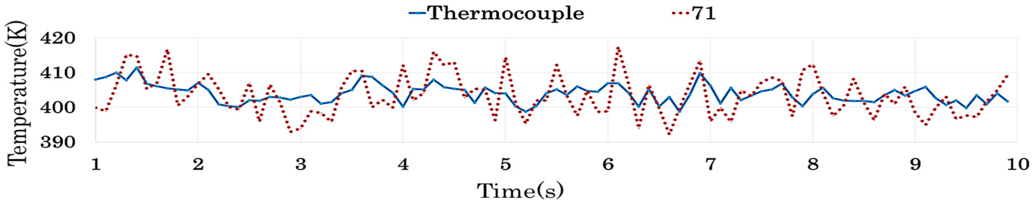
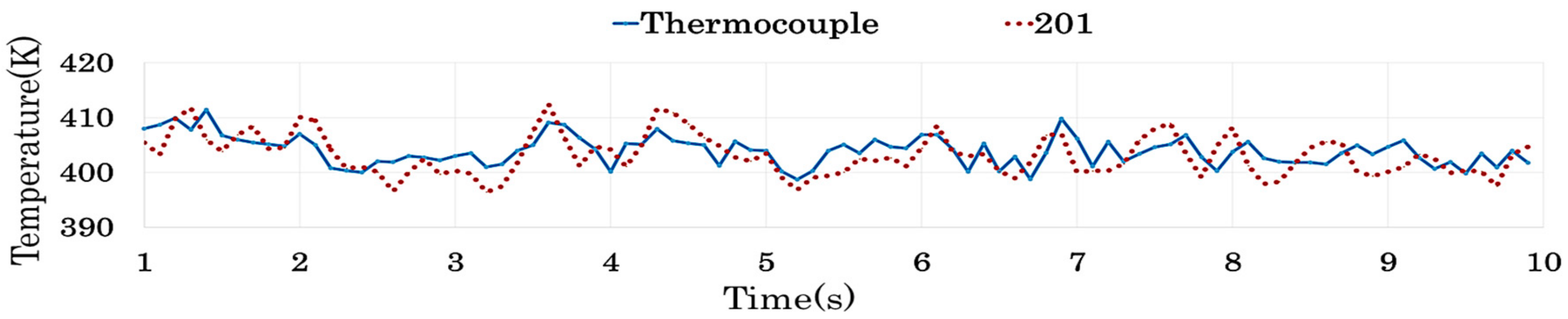
| 806 | 9.9 | 398.712 | 399.182 | 400.164 | 400.543 | |
| 807 | 397.870 | 397.965 | 402.270 | 402.782 | ||
| 808 | 396.147 | 396.544 | 401.184 | 401.859 | ||
| 809 | 397.183 | 397.668 | 401.351 | 401.646 | ||
| 810 | 396.221 | 396.327 | 403.357 | 403.785 | ||
| Time (s) | Test Sets | p-Value | ||
|---|---|---|---|---|
| 1.0 | All sets | <0.05 | ||
| 2.0 | 251 | vs. | 301 | 0.626 |
| 451 | vs. | 501 | 0.476 | |
| 451 | vs. | 601 | 0.402 | |
| 501 | vs. | 601 | 0.331 | |
| 3.0 | All sets | <0.05 | ||
| 4.0 | 351 | vs. | 401 | 0.371 |
| 5.0 | 451 | vs. | 501 | 0.208 |
| 6.0 | 401 | vs. | 451 | 0.633 |
| 7.0 | 601 | vs. | 701 | 0.221 |
| 8.0 | All sets | <0.05 | ||
| 9.0 | All sets | <0.05 | ||
| No. | Group | Time (s) | TThc(i) | ||||
|---|---|---|---|---|---|---|---|
| 31 | 51 | 1001 | |||||
| 1 | 1 | 1.0 | 408.000 | 406.418 | 401.080 | 405.204 | |
| 2 | 1.1 | 408.688 | 402.722 | 401.324 | 406.271 | ||
| 3 | 1.2 | 409.921 | 407.890 | 407.890 | 406.525 | ||
| 4 | 1.3 | 407.798 | 410.285 | 411.842 | 406.990 | ||
| 5 | 1.4 | 411.453 | 402.434 | 411.723 | 406.453 | ||
| 6 | 1.5 | 406.759 | 392.685 | 401.679 | 406.284 | ||
| 7 | 1.6 | 406.005 | 397.013 | 405.508 | 407.419 | ||
| 8 | 1.7 | 405.461 | 418.457 | 416.981 | 407.537 | ||
| 9 | 1.8 | 405.110 | 407.200 | 401.237 | 406.350 | ||
| 10 | 1.9 | 404.842 | 416.607 | 407.599 | 405.416 | ||
| 80 | 9 | 9.0 | 404.658 | 397.217 | 397.462 | 401.795 | |
| 81 | 9.1 | 405.853 | 394.707 | 393.932 | 401.638 | ||
| 82 | 9.2 | 402.657 | 408.041 | 403.190 | 400.741 | ||
| 83 | 9.3 | 400.688 | 395.484 | 396.351 | 400.231 | ||
| 84 | 9.4 | 401.921 | 402.101 | 398.922 | 401.280 | ||
| 85 | 9.5 | 399.798 | 393.647 | 396.263 | 401.277 | ||
| 86 | 9.6 | 403.453 | 410.205 | 399.067 | 401.559 | ||
| 87 | 9.7 | 400.895 | 390.764 | 398.329 | 401.343 | ||
| 89 | 9.8 | 403.987 | 398.441 | 401.295 | 400.894 | ||
| 90 | 9.9 | 401.752 | 403.739 | 409.931 | 400.857 | ||
| Cycles | Time (s) | ||||||||
|---|---|---|---|---|---|---|---|---|---|
| 1 | 2 | 3 | 4 | 5 | 6 | 7 | 8 | 9 | |
| p-Value | |||||||||
| 31 | 0.647 | 0.463 | 0.839 | 0.273 | 0.692 | 0.496 | 0.924 | 0.976 | 0.169 |
| 51 | 0.711 | 0.726 | 0.316 | 0.292 | 0.707 | 0.681 | 0.864 | 0.728 | 0.069 |
| 71 | 0.774 | 0.985 | 0.147 | 0.292 | 0.982 | 0.896 | 0.727 | 0.997 | 0.164 |
| 91 | 0.603 | 0.891 | 0.225 | 0.441 | 0.369 | 0.985 | 0.842 | 0.693 | 0.362 |
| 111 | 0.531 | 0.983 | 0.390 | 0.667 | 0.092 | 0.901 | 0.828 | 0.352 | 0.482 |
| 151 | 0.486 | 0.892 | 0.402 | 0.671 | <0.05 | 0.779 | 0.708 | 0.574 | 0.474 |
| 201 | 0.396 | 0.964 | 0.328 | 0.381 | <0.05 | 0.958 | 0.684 | 0.488 | 0.177 |
| 251 | 0.510 | 0.858 | 0.271 | 0.289 | 0.074 | 0.743 | 0.791 | 0.467 | 0.078 |
| 301 | 0.384 | 0.890 | 0.246 | 0.325 | <0.05 | 0.789 | 0.928 | 0.137 | 0.109 |
| 351 | 0.415 | 0.928 | 0.196 | 0.411 | <0.05 | 0.770 | 0.979 | 0.102 | 0.073 |
| 401 | 0.406 | 0.790 | 0.177 | 0.253 | <0.05 | 0.655 | 0.984 | 0.112 | 0.051 |
| 451 | 0.530 | 0.735 | 0.136 | 0.235 | <0.05 | 0.537 | 0.946 | 0.081 | <0.05 |
| 501 | 0.509 | 0.691 | 0.136 | 0.269 | <0.05 | 0.622 | 0.865 | <0.05 | <0.05 |
| 601 | 0.478 | 0.620 | 0.097 | 0.284 | <0.05 | 0.495 | 0.886 | <0.05 | <0.05 |
| 701 | 0.432 | 0.631 | 0.084 | 0.367 | <0.05 | 0.449 | 0.911 | <0.05 | 0.054 |
| 801 | 0.357 | 0.550 | 0.058 | 0.336 | <0.05 | 0.430 | 0.977 | <0.05 | <0.05 |
| 901 | 0.316 | 0.574 | 0.053 | 0.431 | 0.062 | 0.431 | 0.871 | <0.05 | <0.05 |
| 1001 | 0.216 | 0.528 | <0.05 | 0.446 | 0.057 | 0.413 | 0.773 | <0.05 | <0.05 |
| Cycles | Time (s) | Total | |||||||||
|---|---|---|---|---|---|---|---|---|---|---|---|
| 1 | 2 | 3 | 4 | 5 | 6 | 7 | 8 | 9 | |||
| RMSE | RMSE | Rank | |||||||||
| 31 | 8.487 | 8.039 | 10.325 | 8.441 | 12.622 | 7.869 | 7.320 | 5.887 | 5.887 | 8.578 | 18 |
| 51 | 5.514 | 5.592 | 6.370 | 5.994 | 7.759 | 4.776 | 6.912 | 5.526 | 5.526 | 6.049 | 17 |
| 71 | 6.269 | 4.497 | 5.404 | 6.334 | 5.316 | 6.007 | 6.028 | 4.420 | 4.420 | 5.538 | 16 |
| 91 | 4.879 | 3.775 | 4.331 | 5.559 | 3.894 | 5.921 | 5.073 | 3.620 | 3.620 | 4.822 | 15 |
| 111 | 4.702 | 3.860 | 4.282 | 5.046 | 3.580 | 5.265 | 4.156 | 3.496 | 3.496 | 4.393 | 14 |
| 151 | 3.755 | 3.129 | 4.216 | 4.833 | 3.564 | 2.957 | 4.314 | 4.065 | 4.065 | 3.918 | 13 |
| 201 | 3.177 | 2.978 | 3.349 | 3.376 | 2.900 | 2.529 | 3.810 | 3.736 | 3.736 | 3.199 | 12 |
| 251 | 3.024 | 3.063 | 3.496 | 3.400 | 2.338 | 3.166 | 3.243 | 2.755 | 2.755 | 3.120 | 11 |
| 301 | 2.603 | 2.884 | 3.159 | 2.961 | 2.749 | 2.844 | 2.541 | 2.267 | 2.267 | 2.809 | 10 |
| 351 | 2.056 | 2.733 | 2.799 | 2.686 | 2.955 | 3.333 | 2.529 | 2.099 | 2.099 | 2.703 | 9 |
| 401 | 1.951 | 2.583 | 2.641 | 2.451 | 2.849 | 3.149 | 2.546 | 2.456 | 2.456 | 2.584 | 4 |
| 451 | 2.047 | 2.909 | 2.662 | 2.403 | 2.785 | 3.439 | 2.512 | 2.156 | 2.156 | 2.641 | 7 |
| 501 | 2.433 | 2.580 | 2.703 | 2.278 | 2.894 | 3.543 | 2.433 | 2.140 | 2.140 | 2.643 | 8 |
| 601 | 2.096 | 2.453 | 2.561 | 2.265 | 2.947 | 3.368 | 2.182 | 2.039 | 2.039 | 2.491 | 1 |
| 701 | 2.201 | 2.591 | 2.899 | 2.426 | 2.925 | 3.544 | 1.905 | 1.987 | 1.987 | 2.555 | 3 |
| 801 | 2.209 | 2.318 | 3.055 | 2.629 | 2.771 | 3.492 | 1.907 | 1.870 | 1.870 | 2.549 | 2 |
| 901 | 2.438 | 2.499 | 3.174 | 2.568 | 2.735 | 3.693 | 2.054 | 1.715 | 1.715 | 2.624 | 6 |
| 1001 | 2.434 | 2.270 | 3.438 | 2.576 | 2.693 | 3.606 | 2.041 | 1.660 | 1.660 | 2.597 | 5 |
| Cycles | Time (s) | Total | |||||||||
|---|---|---|---|---|---|---|---|---|---|---|---|
| 1 | 2 | 3 | 4 | 5 | 6 | 7 | 8 | 9 | |||
| TMD | TMD | Rank | |||||||||
| 31 | 1.860 | 1.124 | 1.188 | 1.208 | 1.174 | 1.383 | 0.889 | 0.731 | 0.880 | 1.121 | 4 |
| 51 | 1.758 | 1.079 | 1.279 | 1.267 | 1.204 | 1.253 | 0.910 | 0.854 | 0.876 | 1.136 | 6 |
| 71 | 1.829 | 0.967 | 1.250 | 1.305 | 0.995 | 1.363 | 0.970 | 0.736 | 1.014 | 1.123 | 5 |
| 91 | 1.780 | 0.873 | 1.170 | 1.348 | 1.006 | 1.299 | 0.915 | 0.773 | 1.148 | 1.112 | 3 |
| 111 | 1.777 | 0.770 | 1.155 | 1.307 | 1.022 | 1.304 | 0.921 | 0.835 | 0.962 | 1.082 | 2 |
| 151 | 1.727 | 0.936 | 1.133 | 1.456 | 1.143 | 1.303 | 1.052 | 0.997 | 1.071 | 1.181 | 10 |
| 201 | 2.132 | 0.798 | 1.552 | 0.888 | 1.549 | 0.992 | 0.684 | 0.429 | 0.506 | 0.933 | 1 |
| 251 | 1.675 | 1.277 | 1.391 | 1.273 | 0.965 | 1.361 | 1.016 | 0.812 | 1.163 | 1.190 | 14 |
| 301 | 1.719 | 1.271 | 1.506 | 1.252 | 1.258 | 1.291 | 1.050 | 0.755 | 0.872 | 1.185 | 12 |
| 351 | 1.626 | 1.280 | 1.394 | 1.261 | 1.291 | 1.481 | 0.996 | 0.745 | 0.911 | 1.188 | 13 |
| 401 | 1.708 | 1.297 | 1.477 | 1.273 | 1.363 | 1.263 | 1.046 | 0.911 | 0.993 | 1.237 | 18 |
| 451 | 1.772 | 1.375 | 1.312 | 1.292 | 1.205 | 1.258 | 0.972 | 0.788 | 1.033 | 1.194 | 16 |
| 501 | 1.871 | 1.342 | 1.264 | 1.328 | 1.309 | 1.153 | 0.945 | 0.811 | 1.056 | 1.200 | 17 |
| 601 | 1.880 | 1.373 | 1.262 | 1.439 | 1.320 | 0.981 | 0.997 | 0.726 | 1.098 | 1.191 | 15 |
| 701 | 1.956 | 1.355 | 1.341 | 1.458 | 1.258 | 0.990 | 0.882 | 0.754 | 1.053 | 1.182 | 11 |
| 801 | 2.012 | 1.320 | 1.347 | 1.479 | 1.299 | 0.849 | 0.814 | 0.727 | 1.147 | 1.165 | 8 |
| 901 | 2.061 | 1.319 | 1.411 | 1.400 | 1.246 | 1.055 | 0.779 | 0.693 | 1.138 | 1.177 | 9 |
| 1001 | 2.058 | 1.233 | 1.382 | 1.393 | 1.243 | 1.006 | 0.788 | 0.655 | 1.153 | 1.154 | 7 |
© 2019 by the authors. Licensee MDPI, Basel, Switzerland. This article is an open access article distributed under the terms and conditions of the Creative Commons Attribution (CC BY) license (http://creativecommons.org/licenses/by/4.0/).
Share and Cite
Jang, H.; Choi, D. Similarity Analysis for Time Series-Based 2D Temperature Measurement of Engine Exhaust Gas in TDLAT. Appl. Sci. 2020, 10, 285. https://doi.org/10.3390/app10010285
Jang H, Choi D. Similarity Analysis for Time Series-Based 2D Temperature Measurement of Engine Exhaust Gas in TDLAT. Applied Sciences. 2020; 10(1):285. https://doi.org/10.3390/app10010285
Chicago/Turabian StyleJang, Hyeonae, and Doowon Choi. 2020. "Similarity Analysis for Time Series-Based 2D Temperature Measurement of Engine Exhaust Gas in TDLAT" Applied Sciences 10, no. 1: 285. https://doi.org/10.3390/app10010285
APA StyleJang, H., & Choi, D. (2020). Similarity Analysis for Time Series-Based 2D Temperature Measurement of Engine Exhaust Gas in TDLAT. Applied Sciences, 10(1), 285. https://doi.org/10.3390/app10010285