Learning Low-Dimensional Embeddings of Audio Shingles for Cross-Version Retrieval of Classical Music

Abstract

Cross-version music retrieval aims at identifying all versions of a given piece of music using a short query audio fragment. One previous approach, which is particularly suited for Western classical music, is based on a nearest neighbor search using short sequences of chroma features, also referred to as audio shingles. From the viewpoint of efficiency, indexing and dimensionality reduction are important aspects. In this paper, we extend previous work by adapting two embedding techniques; one is based on classical principle component analysis, and the other is based on neural networks with triplet loss. Furthermore, we report on systematically conducted experiments with Western classical music recordings and discuss the trade-off between retrieval quality and embedding dimensionality. As one main result, we show that, using neural networks, one can reduce the audio shingles from 240 to fewer than 8 dimensions with only a moderate loss in retrieval accuracy. In addition, we present extended experiments with databases of different sizes and different query lengths to test the scalability and generalizability of the dimensionality reduction methods. We also provide a more detailed view into the retrieval problem by analyzing the distances that appear in the nearest neighbor search.

1. Introduction

Large amounts of digitally available music data require efficient retrieval strategies. In recent decades, many systems for music retrieval based on the query-by-example paradigm have been suggested. Given a fragment of a music representation as a query, the task is to automatically retrieve documents from a music database containing parts or aspects that are similar to the query [1,2,3]. One such retrieval scenario is known as audio identification or fingerprinting [4,5,6,7], where the user specifies a query using an excerpt of an audio recording, and the task is to identify the particular audio recording that is the source of the query. A more challenging scenario is cross-version retrieval, including tasks such as audio matching, version identification, or cover song retrieval [7,8,9,10,11,12,13,14,15,16,17,18,19,20,21,22,23,24,25,26,27,28,29,30]. Here, given an excerpt of an audio recording as a query, the goal is to automatically retrieve all recordings in a database that correspond to the same piece of music as the query. Relevant documents may include various interpretations, arrangements, and cover songs of the piece underlying the recording of the query fragment. We focus on such a retrieval scenario in the context of Western classical music, where one typically has many different performances (referred to as versions) of the same piece of music. For example, given a 10 to 30 s fragment of a recording of Beethoven’s Fifth Symphony performed by the Berlin Philharmonic conducted by Karajan, the task is to identify all versions of this symphony in a database, including an interpretation by the New York Philharmonic conducted by Bernstein and an interpretation by the Vienna Philharmonic conducted by Abbado.

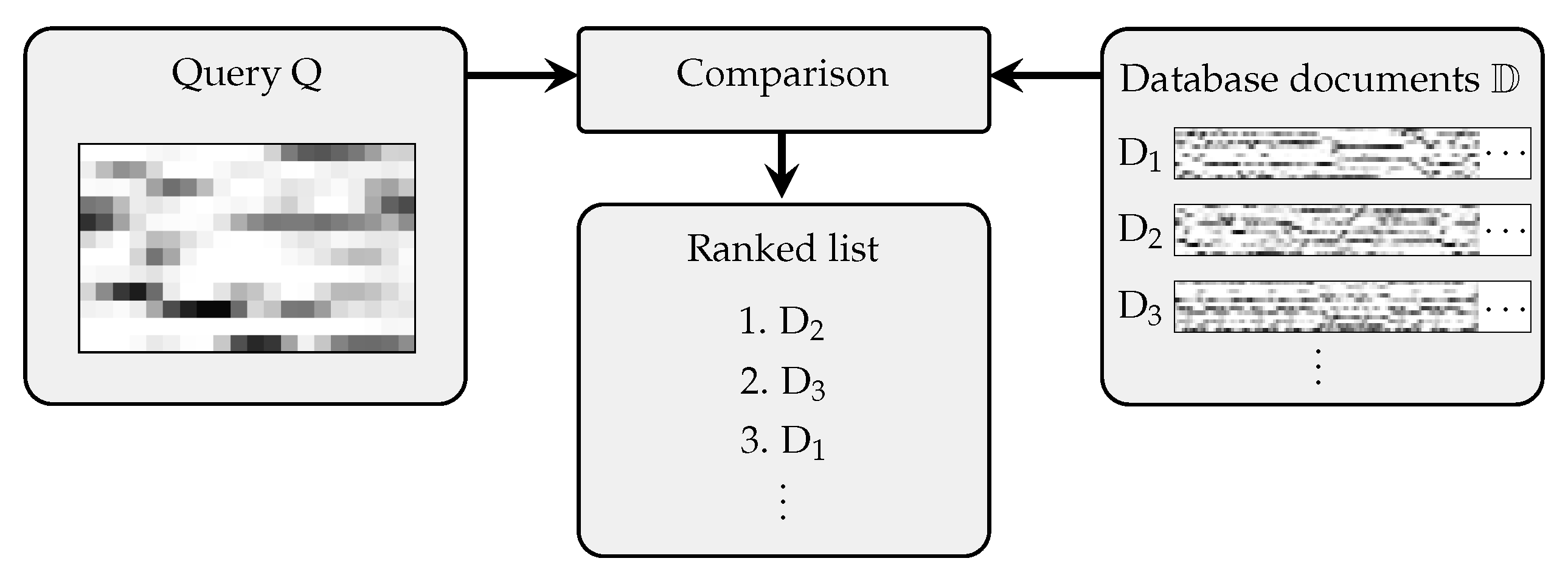
Figure 1 illustrates a typical retrieval procedure, where query and database recordings are compared employing chroma-based audio representations [7] (Chapter 3), resulting in a ranked list of database documents. For comparison, a temporal alignment procedure (e.g., subsequence dynamic time warping [7] (Chapter 7)) is often used to compensate for non-linear tempo differences between the query and relevant database documents [24,31]. However, for huge data collections, the resulting runtime of such approaches is prohibitive. As a more efficient alternative, previous work [1,9,12] introduced shingling approaches, where short feature sequences are used for indexing. In this paper, we build on a study presented by Grosche and Müller [12], who approached this task using chroma-based audio shingles (see the left part of Figure 1 for a visualization of such a shingle). Retrieval was performed via locality-sensitive hashing (LSH) applied to entire shingles. LSH is a random indexing technique for approximate nearest neighbor search [32]. The authors investigated the feature design, the length of the shingles, and the effect of dimensionality reduction applied to individual feature vectors. In this paper, we propose approaches to increase the efficiency of the retrieval even more. We concentrate on the aspect of dimensionality reduction applied to entire shingles so that standard tree-based indexing techniques for nearest neighbor search can be used for retrieval.

As one contribution of this paper, we first use an approach based on principal component analysis (PCA) applied to entire shingles, rather than to individual chroma vectors as in previous work [12]. As another contribution, we then adapt convolutional neural networks with triplet loss [33] to further reduce the shingles’ dimensionality without losing their discriminative power. We conduct basic experiments with a medium-sized collection of music recordings to study the benefits and limitations of the dimensionality reduction methods. As our main result, we show that the shingle dimension can be reduced from 240 to below 8 with only a moderate loss in retrieval quality. Furthermore, we report on extended experiments with a larger data set, using different query lengths to study the scalability and generalizability of the embedding approaches. In our context, scalability refers to the data set size and generalizability refers to the diversity of the data set. We also provide detailed insights into the challenges of the retrieval task and their musical reasons by analyzing the distance distributions that form the basis for the nearest neighbor search.

The structure of this paper is as follows. We give an overview of related work in Section 2 and formalize our retrieval scenario in Section 3. We describe our embedding approaches in Section 4. Then, in Section 5, we report on our basic experiments based on a medium-sized data set. Finally, in Section 6, we give further insights based on our extended experiments using a larger and more diverse data set, and conclude in Section 7 with a short summary.

2. Related Work

On a rough level, we can categorize music retrieval scenarios into metadata- and content-based retrieval tasks [1]. Metadata-based systems use textual information for searching in music databases. On the contrary, content-based systems use actual music data such as sheet music images, symbolic music representations, or audio data. Content-based systems can be further categorized according to the modalities involved. For an overview of multi-modal music retrieval scenarios, we refer to a survey by Müller et al. [34]. In our contribution, we focus on retrieval scenarios, where both query and database documents are audio recordings. In such a setting, we have a query that is either a segment of a music recording or a complete recording. The goal is then to retrieve music recordings that are similar to the query, based on some notion of similarity. Following Casey et al. [1] and Grosche et al. [2], we can categorize such retrieval scenarios according to two properties: Specificity and granularity. Specificity refers to the degree of similarity between the query and the database documents. High specificity is related to a strict notion of similarity, whereas low specificity refers to a rather vague one. The granularity refers to the length of the query, which can range from a short audio snippet (a couple of seconds) to an entire recording (several minutes).

A typical task of high specificity and low granularity is audio identification or audio fingerprinting, where the task is to identify the particular audio recording that is the source of the query [6,35]. At the lower end of the specificity scale are tasks such as genre recognition [36]. A medium-level specificity is associated with tasks such as audio matching [12,14], version identification [31,37], live song detection [28,38], and cover song retrieval [8,10,13,15,16,21,22,23,24,25,26,27,29,30]. In all of these tasks, one allows for variations as they typically occur in different performances and arrangements of a piece of music. The tasks differ in their granularity (e.g., shorter queries for audio matching and longer queries for version identification) and the specific types of music recordings of interest (e.g., live versions by the same performers for live song detection, or popular music with different performers for cover song retrieval). Cover song retrieval is a well-established research task, where one considers variations as they occur in different performances of the same piece of popular music. Such variations concern many different musical facets, including timbre, tempo, timing, structure, key, harmony, and lyrics [25]. A task that is similar to cover song retrieval is version identification for Western classical music, where one allows for variations as they occur in different performances of the same piece of Western classical music [12,14,18,19,20,39,40,41]. This scenario is associated with a higher specificity than cover song retrieval because we expect fewer variations in Western classical music than in popular music. For example, the rough harmonic progression is the same among different performances of the same classical piece, which is not always the case for cover songs of popular music. For that reason, cover song retrieval can be considered a more difficult task compared to version identification for classical music. For more details on this, we refer to the overview article by Serrà et al. [25]. In this paper, we focus on audio matching or version identification for Western classical music.

Miotto and Orio address version identification for classical music by modeling each musical work with a hidden Markov model (HMM) [18,19]. In these studies, a query is identified by choosing the HMM that models the query with the highest probability. To avoid the time-consuming evaluation of all HMMs, the authors propose to first select a small subset of potential candidates [19] and then to evaluate only the HMMs for the most promising candidates. Instead of HMMs, other audio alignment algorithms such as particle filtering have been used in similar settings [20]. Classical music retrieval was also approached as a multi-modal scenario [39,40], in particular using audio and symbolic representations [42]. Arzt et al. [39,40] present an approach that uses symbolic music representations (as the database) to identify a query audio snippet of classical piano music. The query is first transcribed into a series of symbolic events by a neural network. Then, a symbolic fingerprinting algorithm can be applied. This system has a good performance for music where the automatic transcription step achieves good results, e.g., piano music. However, the approach is problematic for kinds of music where automatic transcription is more difficult, such as complex orchestral music. Another line of work uses chroma feature sequences of short audio fragments for audio matching of classical music [12,14]. Our contribution builds upon this line of work and we refer to these studies in the following sections.

3. Shingle-Based Retrieval Scenario

Closely following Grosche and Müller [12], we now formalize the shingle-based retrieval strategy used in this paper. Given a short fragment of a music recording as a query, the goal is to retrieve all versions (documents) of the same piece of music underlying the query. To this end, we compare the database and query recordings based on a particular feature representation. The retrieval result for a query is given as a ranked list of documents. Figure 1 illustrates this general procedure. In the following, we explain the feature computation as well as the retrieval approach.

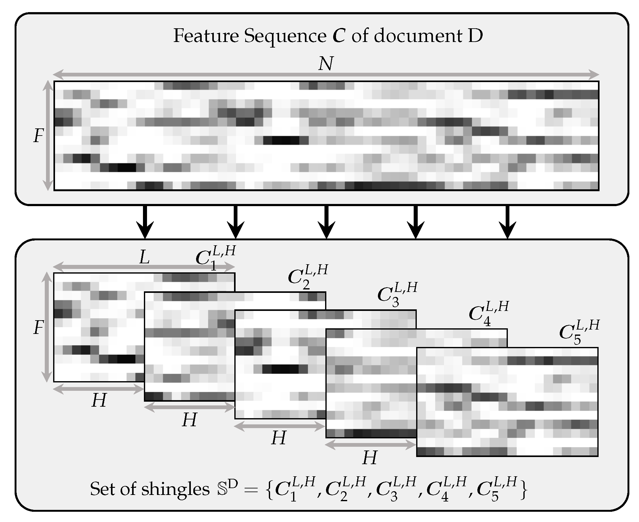
Our approach is based on so-called “shingles” [9], which are short sequences of feature vectors. We denote such a shingle of feature dimension $F\in \mathbb{N}$ and fixed length $L\in \mathbb{N}$ by $\mathit{S}\in {\mathbb{R}}^{F\times L}$. In general, we generate such shingles from audio recordings, which are represented by longer feature sequences of variable length. The feature sequence of an audio recording is denoted by $\mathit{C}=({\mathit{c}}_1,\dots ,{\mathit{c}}_N)$ of length $N\in \mathbb{N}$ and consists of feature vectors ${\mathit{c}}_n\in {\mathbb{R}}^F$ for $n\in \{1,\dots ,N\}$. We use chroma-based audio features, which measure local energy distributions of the audio recording in the $F=12$ chromatic pitch class bands [7] (Chapter 3). More precisely, we use a variant called CENS (chroma energy distribution normalized statistics) [43], which are chroma features with post-processing that makes them more suited for retrieval: First, each chroma vector is ${\ell }^1$-normalized. Then, the resulting values of the chroma features are quantized in a logarithmic way (by mapping logarithmically spaced value ranges to integer values, e.g., values between 0.05 and 0.1 are mapped to to 1, values between 0.1 and 0.2 to 2, etc.). Next, the chroma feature sequence is temporally smoothed (using a smoothing length of 4 s) and downsampled (from 10 Hz to 1 Hz). Finally, each chroma vector is ${\ell }^2$-normalized. The most important aspect of this post-processing is the temporal smoothing, because it makes the features more robust against tempo differences. This chroma variant is state-of-the-art for the given task [12]. The upper part of Figure 2 shows a visualization of the feature type used in this paper. To generate shingles of length $L<N$ from the feature sequence $\mathit{C}$, we use a hop size $H\in \mathbb{N}$ to define the subsequences

$${\mathit{C}}_n^{L,H}:=({\mathit{c}}_{(n-1)H+1},\dots ,{\mathit{c}}_{(n-1)H+L})$$

(1)

for $n\in \{1,\dots ,\lfloor \frac{N-L}{H}\rfloor +1\}$, where $\lfloor ·\rfloor$ denotes the floor operation. The resulting subsequences can also be regarded as matrices or shingles ${\mathit{C}}_n^{L,H}\in {\mathbb{R}}^{F\times L}$. For brevity, we will omit the superscript H in the case of $H=1$. See the lower part of Figure 2 for such a sequence of overlapping shingles.

We now describe the retrieval approach for a fixed query (denoted as $\mathrm{Q}$) and database document (denoted as $\mathrm{D}$). For now, the query consists of a single shingle ${\mathit{S}}^{\mathrm{Q}}\in {\mathbb{R}}^{F\times L}$. Previous investigations of the query length found that a length of 20 s is well suited for performing the retrieval with a single audio shingle [12]. In our study, we use such a shingle length, resulting in a shingle dimensionality of $F\times L=12\times 20=240$. The document $\mathrm{D}$ is represented by a set of shingles

$${\mathbb{S}}^{\mathrm{D}}=\left\{{\mathit{C}}_n^L:n\in \{1,\dots ,N-L+1\}\right\}.$$

(2)

This set ${\mathbb{S}}^{\mathrm{D}}$ consists of all subsequences ${\mathit{C}}_n^L$ from the audio recording of document $\mathrm{D}$ (as defined in Equation (1)), generated with a hop size $H=1$. In the next step, ${\mathit{S}}^{\mathrm{Q}}$ is compared with all shingles from the set ${\mathbb{S}}^{\mathrm{D}}$. The comparison between $\mathrm{Q}$ and $\mathrm{D}$ is achieved by first transforming the shingles to vectors by a function

$$f:{\mathbb{R}}^{F\times L}\to {\mathbb{R}}^K$$

(3)

for some $K\in \mathbb{N}$. In the brute-force case, f just flattens a matrix by concatenating all columns (i.e., $K=FL$). Using shingle embedding methods, as explained later, f performs a dimensionality reduction (typically $K\ll FL$). Given two shingles ${\mathit{S}}^{(1)}$ and ${\mathit{S}}^{(2)}$, we compare them in the embedding space using a distance function

$$d:{\mathbb{R}}^K\times {\mathbb{R}}^K\to {\mathbb{R}}_{\ge 0}.$$

(4)

In the following, we use the squared Euclidean distance:

$$d({\mathit{x}}^{(1)},{\mathit{x}}^{(2)})=\sum _{k=1}^K{(x_k^{(1)}-x_k^{(2)})}^2,$$

(5)

where ${\mathit{x}}^{(1)}=f({\mathit{S}}^{(1)})$ and ${\mathit{x}}^{(2)}=f({\mathit{S}}^{(2)})$. Given a query $\mathrm{Q}$ (in the form of a shingle ${\mathit{S}}^{\mathrm{Q}}$) and a database document $\mathrm{D}$ (in the form of a set of shingles ${\mathbb{S}}^{\mathrm{D}}$), we compute the distance between $\mathrm{Q}$ and $\mathrm{D}$ by

$${\delta }_{\mathrm{D}}({\mathit{S}}^{\mathrm{Q}}):=\underset{\mathit{S}\in {\mathbb{S}}^{\mathrm{D}}}{min}d\left(f({\mathit{S}}^{\mathrm{Q}}),f(\mathit{S})\right).$$

(6)

Finally, for $\mathrm{Q}$ and a data collection $\mathbb{D}$ containing $|\mathbb{D}|$ documents, we compute ${\delta }_{\mathrm{D}}({\mathit{S}}^{\mathrm{Q}})$ between $\mathrm{Q}$ and all $\mathrm{D}\in \mathbb{D}$ and rank the results by ascending ${\delta }_{\mathrm{D}}({\mathit{S}}^{\mathrm{Q}})$.

Previous work [12] used maximum cosine similarity instead of minimum Euclidean distance. We use the squared Euclidean distance because this distance naturally occurs in both dimensionality reduction methods, as explained in Section 4. Note that, since each feature vector of the shingles is normalized, Euclidean distance and cosine similarity lead to similar retrieval results. The relation between the squared Euclidean distance of ${\ell }^2$-normalized vectors and their cosine similarity is given by: $d({\mathit{x}}^{(1)},{\mathit{x}}^{(2)})=2\left(1-cos({\mathit{x}}^{(1)},{\mathit{x}}^{(2)})\right)$.

4. Shingle Embedding

In this section, we explain the brute-force approach and the two shingle embedding techniques. The first uses standard PCA and the second is based on siamese neural networks, which are trained with the so-called triplet loss.

4.1. Brute Force

As a baseline approach, we just flatten each audio shingle $\mathit{S}\in {\mathbb{R}}^{12\times 20}$ to a vector of size $K=12\times 20=240$ by concatenating the feature vectors. In other words, we do not apply any dimensionality reduction. Note that no training is involved in this approach, contrary to the embedding methods that are explained in the following subsections. This baseline approach of using the full-dimensional audio shingles was also used in the study by Grosche and Müller [12].

4.2. PCA

As a first embedding approach, we use PCA [44] to reduce the dimensionality of the audio shingles. Each audio shingle $\mathit{S}\in {\mathbb{R}}^{12\times 20}$ is seen as a vector of size $12\times 20=240$. PCA learns a basis that is used to linearly project these audio shingles. Dimensionality reduction is then performed by considering only the first basis vectors instead of the complete set of basis vectors. This basis is learned such that the squared Euclidean distance between the original and the dimensionality-reduced shingles of a given training set is minimized. As a result, one obtains a linear transformation that maps an audio shingle $\mathit{S}$ to an embedding vector $\mathit{x}\in {\mathbb{R}}^K$. This mapping $f(\mathit{S})=\mathit{x}$ is then used in the experiments with a separate test set by embedding the entire database as well as the queries before performing the retrieval (see Section 5.4). The authors of [12] also used PCA for dimensionality reduction, but they applied PCA only to individual chroma vectors of dimension F. Thus, their approach can only make use of the chroma dimension, without any temporal information. In our approach, we apply PCA to entire shingles of dimension $F\times L$ and can, therefore, exploit redundancies in the temporal sequence of chroma vectors for dimensionality reduction.

4.3. Neural Network with Triplet Loss

As a second embedding approach, we use neural networks to reduce the dimensionality of the audio shingles. Such networks can be used to learn non-linear functions that map high-dimensional input representations to low-dimensional output representations. We now show how the dimensionality of the audio shingles can be reduced using a convolutional neural network trained with the triplet loss [33]. During training, our network embeds three shingles for computing the loss, which is then used for updating the parameters of the network. This will be explained in detail later in this section. Figure 3 shows an illustration of this process.

For learning embeddings, a loss function that enforces specified similarities and dissimilarities in the embedding space is used. An example of such a loss function is the hinge loss, which has been used to learn representations for cross-modal score-to-audio embeddings [45] and for artist similarity [46]. A related loss function is the triplet loss, which was developed for the task of face recognition [33] and then adapted for audio and music processing tasks such as speech retrieval [47], sound event classification [48], audio fingerprinting [49], artist clustering [50], music similarity [51], and cover song retrieval [37]. The latter study is conceptually similar to our approach, but presents results that are worse than those achieved by more traditional approaches [21].

To define the triplet loss in our scenario, we select three shingles: An anchor shingle ${\mathit{S}}^{\mathrm{a}}$, a positive shingle ${\mathit{S}}^{\mathrm{p}}$, and a negative shingle ${\mathit{S}}^{\mathrm{n}}$ (see the upper part of Figure 3 for an example). With respect to the anchor shingle, the positive shingle is musically similar, while the negative shingle is musically dissimilar. More precisely, the anchor and positive shingles originate from different versions of the same piece of music and correspond to the same musical position within that piece. Anchor and negative shingles do not correspond to each other.

The goal is to find an embedding function $f:{\mathbb{R}}^{F\times L}\to {\mathbb{R}}^K$ such that $f({\mathit{S}}^{\mathrm{a}})$ is numerically close to $f({\mathit{S}}^{\mathrm{p}})$ and far from $f({\mathit{S}}^{\mathrm{n}})$. The lower part of Figure 3 visualizes embeddings with this property. Let

$$\mathit{X}=\left({\mathit{x}}^{\mathrm{a}},{\mathit{x}}^{\mathrm{p}},{\mathit{x}}^{\mathrm{n}}\right)=\left(f\left({\mathit{S}}^{\mathrm{a}}\right),f\left({\mathit{S}}^{\mathrm{p}}\right),f\left({\mathit{S}}^{\mathrm{n}}\right)\right).$$

(7)

Then, following Schroff et al. [33], we define the loss as

$$\mathcal{L}(\mathit{X})=max\left(0,d({\mathit{x}}^{\mathrm{a}},{\mathit{x}}^{\mathrm{p}})-d({\mathit{x}}^{\mathrm{a}},{\mathit{x}}^{\mathrm{n}})+\alpha \right),$$

(8)

with $\alpha \in {\mathbb{R}}_{\ge 0}$ being a margin parameter and d being a distance function. In our experiments, we use the squared Euclidean distance, as defined in Equation (5). The cost function J to be optimized during batch gradient descent is the average of losses over a batch $\mathbb{B}$ of triplets:

$$J(\mathbb{B})=\frac{1}{|\mathbb{B}|}\sum _{\mathit{X}\in \mathbb{B}}\mathcal{L}(\mathit{X}).$$

(9)

Our neural network architecture is summarized in

Table 1. Neural network architecture. For all convolutional operations, we use a zero-padding size of 1. Conv2D* indicates a circular padding of the chroma axis instead of zero-padding.

Layer	Output Shape	Parameters
Input	(12, 20, 1)
Conv2D* 12×(3, 3, 1)	(12, 20, 12)	108
BatchNorm + ELU	(12, 20, 12)	48
Conv2D 12×(3, 3, 12)	(12, 20, 12)	1296
BatchNorm + ELU	(12, 20, 12)	48
MaxPool2D (2, 2)	(6, 10, 12)
Conv2D 12×(3, 3, 12)	(6, 10, 12)	1296
BatchNorm + ELU	(6, 10, 12)	48
Conv2D 12×(3, 3, 12)	(6, 10, 12)	1296
BatchNorm + ELU	(6, 10, 12)	48
MaxPool2D (2, 2)	(3, 5, 12)
Flatten + Dense K	(K)	$K\times$ 181
Output: ${\ell }^2$-normalize	(K)

. It comprises two blocks, each consisting of two convolutional layers and a max-pooling layer. Finally, a dense layer reduces the network’s internal representation to the embedding dimensionality K; an ${\ell }^2$-normalization layer ensures that the embedding vectors do not become arbitrarily large or small. This topology is inspired by a network for multi-modal music embeddings [45]. We simplified the architecture (e.g., using 2 blocks instead of 4) for two reasons: First, our scenario is mono-modal and therefore less complex compared to the multi-modal task [45], and second, our input dimension is smaller (using chroma features instead of spectral features). Our network has relatively few parameters compared with many other deep learning systems. E.g., for $K=10$, the network has about 6000 parameters.

5. Basic Experiments

In this section, we report on our experiments with medium-sized data sets for training and testing. Later, in Section 6, we will also report on experiments with an extended data set. For now, we use medium-sized data sets similar to those used in previous studies [12] for being comparable with this work. First, we describe the data sets and our evaluation measures. Second, we discuss the evaluation results obtained using the brute-force approach, the PCA-based embeddings, and the approach using neural networks. Third, we analyze the influence of the margin parameter $\alpha$ (used in the loss function) on the retrieval results. Finally, we report on a runtime experiment that indicates the impact of the embeddings’ dimensionality on the retrieval time.

5.1. Training and Testing Data Sets

In our experiments, we used audio recordings of Western classical music. In particular, we used pieces from three composers: Symphonies by Beethoven, Mazurkas by Chopin, and pieces from Vivaldi’s The Four Seasons. These composers cover three different musical eras, namely the Baroque, Classical, and Romantic periods.

Table 2. The music collections ${\mathbb{D}}_1$ used for training and ${\mathbb{D}}_2$ used for testing. Duration format hh:mm:ss.

	Composer	Piece	Genre	Versions	Dur	⌀ Dur
Training set${\mathbb{D}}_{\mathbf{1}}$	Beethoven	Op. 67, Mov. 1	symphony	10	1:12:07	0:07:13
		Op. 67, Mov. 2		10	1:44:53	0:10:29
		Op. 67, Mov. 3		10	1:02:53	0:06:17
		Op. 67, Mov. 4		10	1:48:00	0:10:48
	Chopin	Op. 17, No. 4	mazurka (piano solo)	62	4:29:23	0:04:21
		Op. 24, No. 2		64	2:26:38	0:02:17
		Op. 30, No. 2		33	0:46:52	0:01:25
		Op. 63, No. 3		86	3:05:06	0:02:09
		Op. 68, No. 3		51	1:25:58	0:01:41
	Vivaldi	RV 315, Mov. 1	violin concerto	7	0:37:40	0:05:23
		RV 315, Mov. 2		7	0:17:23	0:02:29
		RV 315, Mov. 3		7	0:20:40	0:02:57
	$\mathsf{\Sigma }$			357	19:17:32
Test set${\mathbb{D}}_{\mathbf{2}}$	Beethoven	Op. 55, Mov. 1	symphony	4	1:06:34	0:16:38
		Op. 55, Mov. 2		4	1:02:52	0:15:43
		Op. 55, Mov. 3		4	0:23:41	0:05:55
		Op. 55, Mov. 4		4	0:46:07	0:11:32
	Chopin	Op. 7, No. 1	mazurka (piano solo)	53	2:01:15	0:02:17
		Op. 24, No. 1		61	2:53:48	0:02:51
		Op. 33, No. 2		67	2:40:38	0:02:24
		Op. 33, No. 3		50	1:29:22	0:01:47
		Op. 68, No. 4		62	2:33:58	0:02:29
	Vivaldi	RV 269, Mov. 1	violin concerto	7	0:24:17	0:03:28
		RV 269, Mov. 2		7	0:20:20	0:02:54
		RV 269, Mov. 3		7	0:30:46	0:04:24
	$\mathsf{\Sigma }$			330	16:13:37

shows a list of the musical pieces underlying the recordings. For each musical piece, our database contains several versions that are performed by different orchestras, conductors, and soloists. To make our results comparable to prior work, we use audio data sets that are similar to the one used in the study by Grosche and Müller [12]. The data sets comprise recordings of some of Frédéric Chopin’s Mazurkas, which have been collected within the Mazurka Project [52].

There are two disjoint sets: ${\mathbb{D}}_1$ (357 recordings, 62,867 shingles) was used for training the dimensionality reduction methods, and ${\mathbb{D}}_2$ (330 recordings, 52,332 shingles) was used for evaluating the retrieval quality based on the embedded shingles. Furthermore, circular chroma shifts were applied to the training set, which simulate musical transpositions and increase the number of shingles used for training by a factor of twelve. This process can be seen as a type of data augmentation. Both training and test sets are musically related, as they contain the same composers and the same music genres. However, the musical pieces in both sets are different.

5.2. Evaluation Procedure

In our testing stage, we used the data set ${\mathbb{D}}_2$, which is independent of the training set ${\mathbb{D}}_1$. When performing retrieval using a query $\mathrm{Q}$, we computed ${\delta }_{\mathrm{D}}({\mathit{S}}^{\mathrm{Q}})$ for all $\mathrm{D}\in {\mathbb{D}}_2$ and obtained a ranked list of documents, as described in Section 3. We excluded the document containing the query from the database ${\mathbb{D}}_2$ so that there are no trivial retrieval results.

For evaluating the results, we considered three evaluation measures. First, we used precision at one (P@1), which is 1 if the top-ranked document is relevant, and 0 otherwise. However, not only the top rank is of relevance in our retrieval scenario. This was taken into account by our second evaluation measure, called R-precision (P${}_R$). Here, $R\in \mathbb{N}$ denotes the number of relevant documents for a given query. Note that this number may be different for different queries. P${}_R$ is defined as the proportion of relevant documents among the first R ranks. Third, we used average precision, which is a standard evaluation measure for information retrieval that takes the entire list of ranks into account. It is defined as the mean of the precision scores for the ranks with retrieved relevant documents. This measure is not as well interpretable as P@1 or P${}_R$, but it is the most comprehensive evaluation measure that we used. For a more detailed explanation, we refer to the book by Manning et al. [53] (Chapter 8).

For our experiments, we used a set of queries, which we created by equidistantly sampling 10 queries from each recording of our test set ${\mathbb{D}}_2$, resulting in 3300 queries. The evaluation results were then averaged over all queries. In the case of average precision, the averaged measure is referred to as mean average precision (MAP).

5.3. Brute Force

As a baseline, we performed a first retrieval experiment based on the original audio shingles without dimensionality reduction (see Section 4.1). Since no training was involved, we report the results in

Table 3. Retrieval results for various brute-force approaches: The shingle-based brute-force approach ($K=240$), an alignment-based brute-force approach using chroma energy distribution normalized statistics (CENS) features (1 Hz), and an alignment-based brute-force approach using chroma features (10 Hz) without CENS post-processing.

Brute-Force Approach	Data Set	P@1	P${}_{\mathit{R}}$	MAP
Shingles ($K=240$)	${\mathbb{D}}_1$	0.993	0.936	0.966
	${\mathbb{D}}_2$	0.996	0.941	0.972
SDTW (CENS, 1 Hz)	${\mathbb{D}}_1$	0.991	0.947	0.971
	${\mathbb{D}}_2$	0.994	0.947	0.975
SDTW (Chroma, 10 Hz)	${\mathbb{D}}_1$	0.995	0.966	0.980
	${\mathbb{D}}_2$	0.999	0.978	0.989

(upper rows) for both the training set ${\mathbb{D}}_1$ and the test set ${\mathbb{D}}_2$. For example, in the case of the test set ${\mathbb{D}}_2$, we achieved a P@1 value of 0.996, which means that only 13 of the 3300 queries did not yield a relevant document on the top rank. Furthermore, the MAP value of 0.972 indicates that almost all relevant documents appear at the beginning of the ranked list. The results for the training set are similar, indicating a comparable complexity of both data sets.

The parameters and feature design of the shingles were chosen in such a way that the brute-force approach yielded close to perfect results for the given task. For a comparison, we also performed an experiment using a temporal alignment procedure, similar to the classical state-of-the-art approaches for cover song retrieval by Serrà et al. [24,25,54]. In essence, these approaches are based on the combination of enhanced chroma representations with non-linear temporal alignment procedures. In our experiments, we performed subsequence dynamic time warping (SDTW) [7] (Chapter 7) to align the feature sequences of a query and a database document. The approaches of Serrà et al. [24,54] used local alignment procedures that aligned subsequences of the query to subsequences of the database document (e.g., Smith–Waterman, or $Q_{\max }$ algorithm). This was motivated by the task of popular music cover song retrieval where the query is a complete recording. In this case, query and relevant database documents typically have a different structure. However, in our case, we are dealing with Western classical music, and the query is only a 20 s excerpt. Therefore, we can expect that the query is entirely represented as a musically corresponding subsequence in the relevant database documents. Under this assumption, SDTW is more or less equivalent to the Smith–Waterman algorithm. For SDTW, we used the Euclidean distance, the step size condition $\{(2,1),(1,2),(1,1)\}$, and the weights $(2,1,1)$ for vertical, horizontal, and diagonal steps, respectively. As a result of SDTW, we obtained a matching function; the minimum of this matching function was used as a distance measure for ranking the documents. Table 3 (middle rows) shows the retrieval results for this experiment, using the CENS features described in Section 3. These results are very close to the results of the shingle-based brute-force approach. This confirms that in our music scenario, no alignment procedure is needed when using CENS processing.

One main motivation for using CENS smoothing is to introduce robustness to local tempo variations. When an alignment procedure is used, such smoothing is not needed. Therefore, we also conducted an alignment experiment, using the original chroma features without CENS post-processing. In this setting, the feature rate was 10 Hz instead of 1 Hz. Table 3 (lower rows) shows the retrieval results using these features. In the case of the test set ${\mathbb{D}}_2$, we achieved a P@1-value of 0.999, which means that almost all queries yielded a relevant document on the top rank. In all evaluation measures, we see small improvements over the shingle-based brute-force approach. However, this goes along with a dramatic increase in runtime. The runtime for the overall retrieval experiment in our setting increased from about a minute for the shingle-based brute-force approach (1 Hz features) to several hours for the alignment-based approach using 10 Hz features. We describe further aspects related to runtime in Section 5.7.

In summary, we showed that we can get close-to-perfect results with the brute-force approaches. In other words, when only looking at retrieval quality, the problem of cross-version retrieval for Western classical music can be regarded as being largely solved. However, brute-force approaches are time-consuming. The main focus of this paper is efficiency, and we want to see to which extent we can keep the retrieval quality while reducing the shingle dimensionality. Therefore, in the following, we are not aiming for improving the brute-force approaches, but for keeping a comparable result while using low-dimensional embeddings of the audio shingles. If not mentioned otherwise, brute-force always refers to the shingle-based brute-force approach in the following.

5.4. PCA

As the second approach, we applied dimensionality reduction with PCA as described in Section 4.2. We used the training set ${\mathbb{D}}_1$ to learn the PCA basis and evaluate the approach with the test set ${\mathbb{D}}_2$.

Table 4. Retrieval results for principle component analysis (PCA)-based dimensionality reduction of individual chroma vectors (GRO) [12] and entire shingles (PCA, proposed) using the test set ${\mathbb{D}}_2$.

		GRO [12]				PCA
K		P@1	P${}_{\mathit{R}}$	MAP		P@1	P${}_{\mathit{R}}$	MAP
40		0.930	0.773	0.832		0.991	0.926	0.964
60		0.975	0.871	0.921		0.993	0.938	0.971
80		0.987	0.903	0.948		0.994	0.942	0.973

shows the evaluation results for two different PCA-based reduction strategies: The left columns (GRO) refer to the reduction of individual chroma vectors as done by Grosche and Müller [12], and the right columns (PCA) refer to the proposed reduction of entire shingles. The rows correspond to the considered dimensionalities 40, 60, and 80. Let us take the case of $K=40$ as an example. In the first approach (GRO), each chroma vector was reduced to two dimensions, leading to the dimensionality of $K=2\times 20=40$. This strategy resulted in an MAP value of 0.832. In the shingle-based reduction (PCA), an entire 240-dimensional feature sequence was reduced altogether to a 40-dimensional vector. This approach led to an MAP value of 0.964. In general, our experiments showed that a shingle-based reduction leads to better retrieval results. This is not surprising, because this approach can exploit temporal redundancies for dimensionality reduction. In the following, we aim to reduce the dimensionality to a degree that would not have been possible with the first approach (GRO). Columns 2–4 of

Table 5. Retrieval results for our proposed PCA- and DNN-based dimensionality reduction methods using the test set ${\mathbb{D}}_2$.

		PCA				DNN
K		P@1	P${}_{\mathit{R}}$	MAP		P@1	P${}_{\mathit{R}}$	MAP
3		0.603	0.550	0.580		0.671	0.647	0.683
4		0.807	0.714	0.754		0.772	0.718	0.755
5		0.830	0.712	0.758		0.821	0.766	0.806
6		0.857	0.724	0.771		0.890	0.816	0.856
7		0.888	0.739	0.790		0.908	0.827	0.869
8		0.904	0.754	0.806		0.936	0.856	0.898
9		0.927	0.778	0.834		0.946	0.867	0.910
10		0.945	0.811	0.868		0.954	0.877	0.919
11		0.951	0.813	0.872		0.957	0.888	0.927
12		0.957	0.819	0.877		0.964	0.887	0.928
15		0.974	0.846	0.904		0.969	0.901	0.940
20		0.985	0.878	0.932		0.970	0.905	0.942
30		0.990	0.908	0.952		0.981	0.927	0.959

show the evaluation results obtained with our shingle-based approach for much lower dimensionalities. The retrieval quality consistently increases with an increase of dimensionality from an MAP value of 0.580 for $K=3$ to 0.952 for $K=30$. Let us consider the dimensionalities of 6 and 12 as exemplary cases. For $K=6$ the P@1 value is 0.857, i.e., for 472 of the 3300 queries, the top-ranked document was not relevant. For $K=12$ (P@1: 0.957), this is the case for only 142 queries.

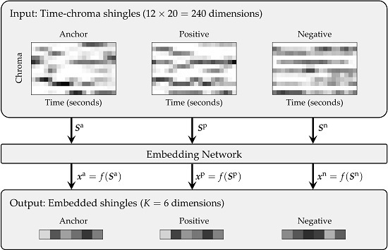
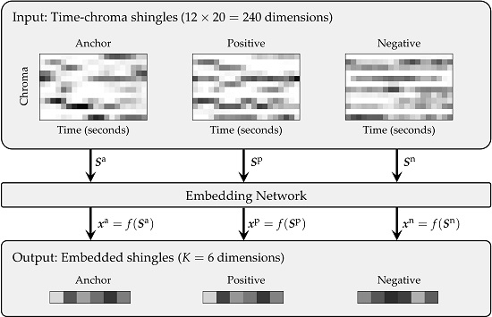
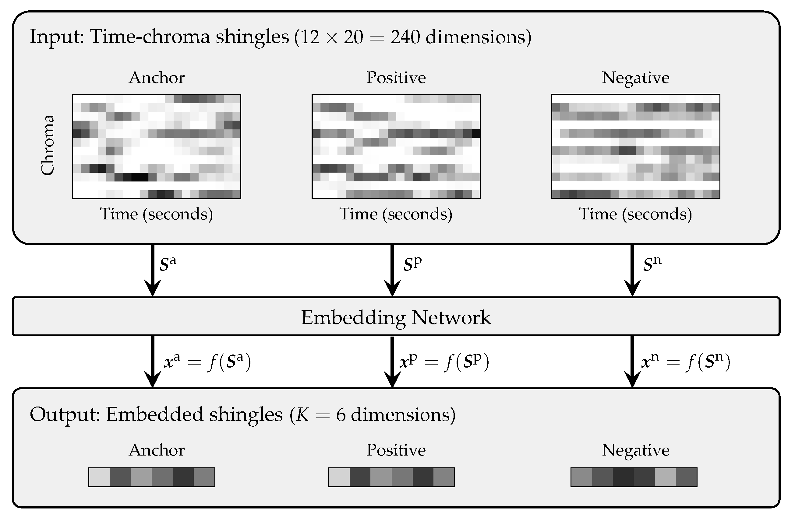
5.5. Neural Network with Triplet Loss

As the third approach, we applied dimensionality reduction with a deep neural network (DNN) as described in Section 4.3. For training the neural network, we used triplets of shingles from the training set ${\mathbb{D}}_1$. They were generated with the constraint that the central time positions of the anchor and positive shingles corresponded to the same musical position in different versions of the same piece. The negative shingle did not musically correspond to the anchor shingle. To generate such musically meaningful triplets, we needed to compute musically corresponding time positions in all versions of the same pieces in a pre-processing stage. We used a dynamic-time-warping-based music synchronization approach [7] (Chapter 3) for this purpose. Furthermore, random circular shifts along the chroma axis were applied to avoid biasing the network towards the musical keys in our data set. The shifts applied to the anchor and the positive examples were the same, while the shift applied to the negative example was chosen independently. This triplet generation procedure led to a combinatorial explosion of possible triplets. For that reason, not all possible triplets were provided to the network during training. We defined an “epoch” to consist of 2000 batches with a batch size of 128 triplets, used for batch gradient descent with the Adam optimizer [55]. Other triplet loss studies sometimes control the triplet generation by a specific procedure called “semi-hard triplet mining” [33]. Preliminary experiments (not reported here) showed that in our case, there were no improvements by this method. Therefore, we do not apply this procedure in the experiments reported in this paper. In our first experiments, we fixed $\alpha =1.3$ (see Section 5.6 for a discussion) as well as a learning rate of ${10}^{-3}$ and trained a neural network for 10 epochs. It turned out that a larger number of epochs did not improve the retrieval results.

Columns 5–7 of Table 5 show the evaluation results for a range of different dimensionalities from 3 to 30 using the test set ${\mathbb{D}}_2$. In general, the retrieval quality increases with an increase of K from an MAP value of 0.683 for $K=3$ to 0.959 for $K=30$. Let us consider some cases as examples. For $K=6$, the P@1 value is 0.890, i.e., for 363 of the 3300 queries, the top-ranked document was not relevant. For $K=12$ (P@1: 0.964), this is the case for only 119 queries. Compared to the PCA-based approach, the neural network especially improved the retrieval results for smaller dimensionalities like 6 or 8, where the MAP value is greater by more than 0.08 (e.g., $K=8$, MAP for PCA: 0.806 and for DNN: 0.898). We observed rather small improvements in P@1, but there was a considerable increase of P${}_R$ (e.g., $K=8$, P${}_R$ for PCA: 0.754 and for DNN: 0.856).

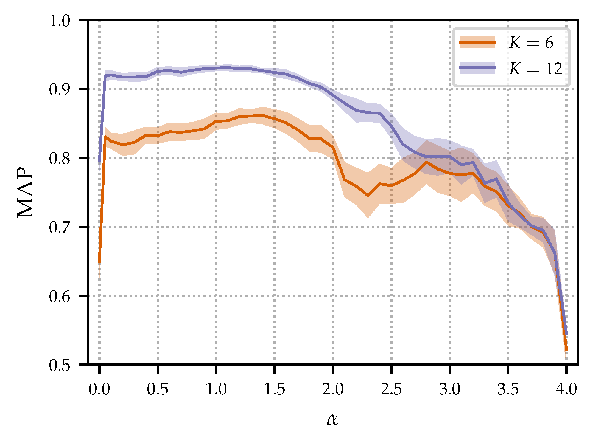
5.6. Influence of $\alpha$

In the following, we analyze the influence of the parameter $\alpha$, which is used in the loss function as defined in Equation (8). This parameter can be interpreted as the margin between $d({\mathit{x}}^{\mathrm{a}},{\mathit{x}}^{\mathrm{p}})$ and $d({\mathit{x}}^{\mathrm{a}},{\mathit{x}}^{\mathrm{n}})$. Figure 4 shows the evaluation results (MAP) for various $\alpha$ values. For this experiment, we only used the dimensionalities of $K=6$ and $K=12$ as examples to illustrate general tendencies. For a given $\alpha$ and K, 25 neural networks were trained for 10 epochs with different random initializations. Then, they were used for dimensionality reduction in the retrieval scenario, resulting in 25 MAP values. From these, we computed the mean ($\mu$) and the standard deviation ($\sigma$). The solid lines show $\mu$ and the light areas show $\pm \sigma$ around $\mu$. For both $K=6$ and $K=12$, we see similar trends: $\alpha =0$ achieves rather bad results. In this case, no margin is enforced, and the loss is zero as soon as $d({\mathit{x}}^{\mathrm{a}},{\mathit{x}}^{\mathrm{p}})\le d({\mathit{x}}^{\mathrm{a}},{\mathit{x}}^{\mathrm{n}})$. However, increasing $\alpha$ only slightly leads to a clear improvement in MAP. Any $\alpha$ in the range of $[0.1,1.7]$ produces results of similar quality. For $\alpha >1.7$, the results strongly decrease. This can be explained as follows: Only a small positive margin is needed for retrieving the correct versions. Using a large margin brings no benefit for retrieval, but makes the training much harder. In summary, for $0.1\le \alpha \le 1.7$, we see a stable overall behavior of the results with a small standard deviation, showing robustness to the initialization used.

5.7. Runtime Experiment

We showed that we can substantially reduce the dimensionality of the audio shingles while keeping their discriminative power. Such low-dimensional embeddings are beneficial when using indexing techniques for efficient nearest neighbor retrieval. To show this property, we conducted an experiment where we computed the distances of the 3300 queries to the documents of our test set ${\mathbb{D}}_2$ (as done for the previous experiments). We measured the runtimes for the alignment-based approaches (described in Section 5.3) and for the shingle-based approaches. In the case of the shingle-based approaches, we employed three different nearest neighbor search strategies. The first search strategy is a full search by just computing all distances between the shingles of the database documents and the query shingles. For the second and third search strategies, we used k-d trees, which are standard data structures for searching in multidimensional spaces [56]. In the second strategy (Doc-Trees), we built one tree for each of the 330 documents of the test set and searched for the nearest neighbor to the query in each tree. As a consequence, each document occurred precisely once in the ranked list (as in the previous experiments). In the third strategy (Db-Tree), we built a single tree for all documents of the database and searched for the 330 nearest embeddings to the query. With this strategy, we were not able to rank all documents of the database because some of the returned embeddings originated from the same document. Note that the reported runtimes depend on the used implementations. So, rather than focusing on the absolute times, we want to emphasize the relative tendencies as well as the orders of magnitude.

We performed our experiments using Python 3.6.5 on a computer with an Intel Xeon CPU E5-2620 v4 (2.10 GHz) and 31GiB RAM. For the alignment-based approaches, we used the SDTW implementation of librosa 0.7.1 [57], which is written in Python and accelerated by the just-in-time compiler numba. For the full search, we used the efficient pairwise-distance calculation of scipy 1.0.1 [58], which calls a highly optimized implementation in C. For the k-d trees (using a default leaf size of 30), we used the implementation of scikit-learn 0.20.1 [59], which is written in Cython.

Table 6. Time (in seconds) needed for searching 3300 queries, for selected approaches.

Approach	Full Search	Index (Db-Tree)
Brute Force, SDTW (Chroma, 10 Hz)	23,190.1	-
Brute Force, SDTW (CENS, 1 Hz)	351.5	-
Brute Force, Shingles ($K=240$)	23.0	76.9
DNN ($K=30$)	3.3	5.0
DNN ($K=12$)	1.8	1.1
DNN ($K=6$)	1.2	0.4

presents the runtimes for selected settings, averaged over several iterations of the retrieval experiment. The first column specifies the retrieval approach, the second column lists the runtimes for the full search strategy, and the third column lists the runtimes for the Db-Tree search strategy. For the alignment-based approach using 10 Hz features (first row), the runtime was about 6.5 h. When using 1 Hz features (second row), the runtime decreased to about 6 minutes. It is not surprising that the first alignment-based approach was much slower, since the feature rate was ten times higher and the alignment algorithms were of quadratic complexity. For the brute-force shingle approach ($K=240$, third row), the runtime was significantly lower than for both alignment-based approaches. It took 23.0 s for the full search strategy and 76.9 s for the Db-Tree search strategy. In our setting and with the used implementations, the Db-Tree strategy was slower than full search for $K=240$. It is well known that k-d trees degenerate for high dimensions [60]. With dimensionality reduction to $K=30$ or $K=12$ (fourth and fifth row), both search strategies were in a similar range (e.g., for $K=12$, full search: 1.8 s, Db-Tree: 1.1 s). For lower dimensions ($K=6$, sixth row), the Db-Tree search strategy substantially accelerated the nearest neighbor search (full search: 1.2 s, Db-Tree: 0.4 s).

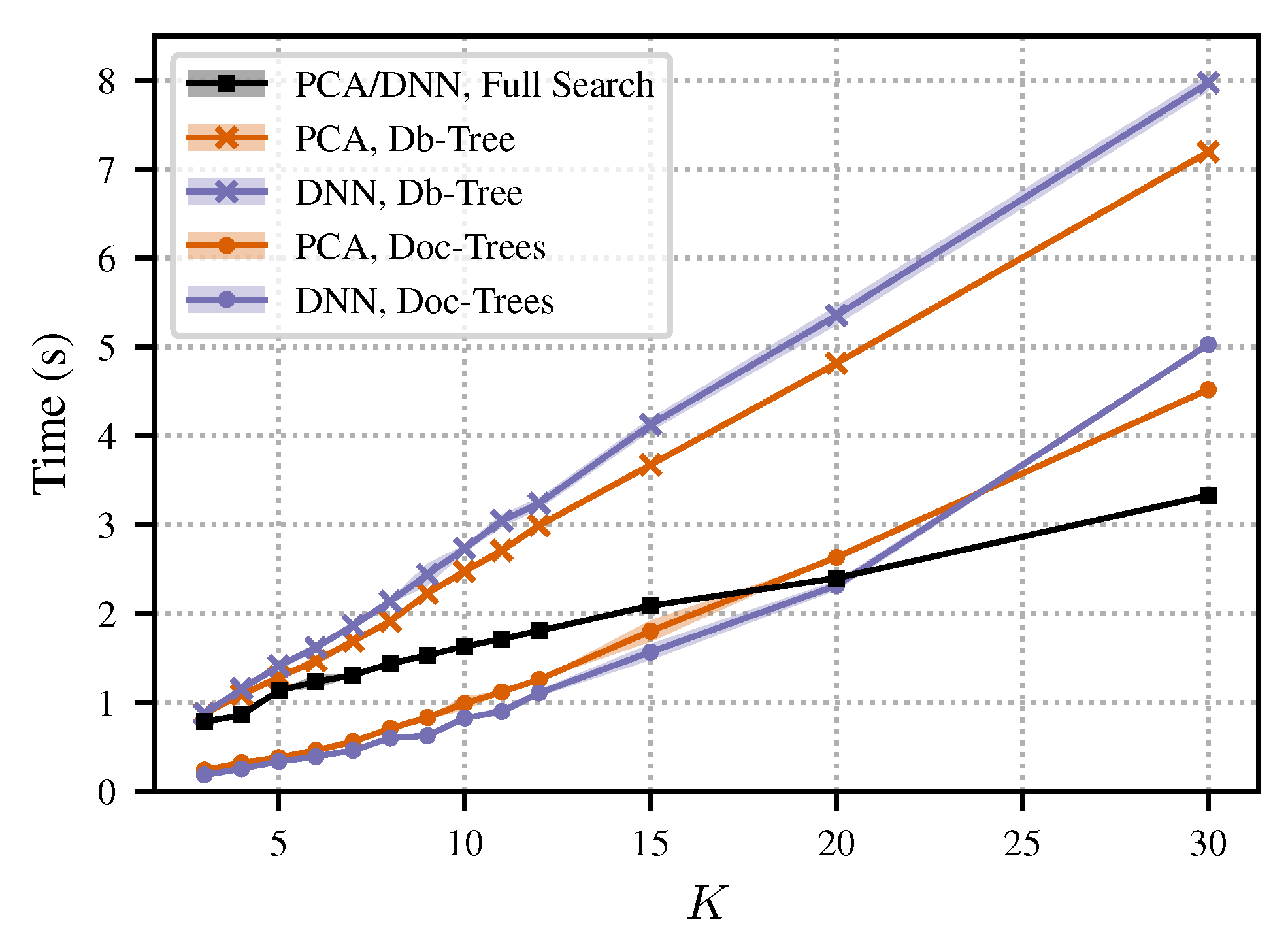
Figure 5 shows the runtime ($\mu$ and $\pm \sigma$ for 100 iterations of the retrieval experiment) for the dimensionality reduction approaches. For the full search strategy, we see an almost linear relationship between the dimensionality K and the runtime. This strategy is independent of the underlying data distribution. For that reason, we do not distinguish between PCA- and DNN-based dimensionality reduction for the full search strategy. This is different for the tree-based search strategies (Db-Tree and Doc-Trees), where the data distributions of the PCA- and DNN-based embeddings lead to different search times. We also see an almost linear relationship for the Doc-Trees search strategy for both PCA- and DNN-based retrieval approaches. In general, for this strategy, the runtime is higher than for the full search. In our case, the data size of a single document is too small for the Doc-Trees strategy to give any benefit over the full search strategy. For the Db-Tree strategy, we see a slightly exponential growth of runtime with growing K. When the dimensionality falls below 15, the Db-Tree strategy starts to give benefits for the fast nearest neighbor search.

We want to emphasize again that the absolute runtimes are implementation-dependent. Therefore, we want to highlight some general tendencies: The shingle-based approaches are significantly faster than the alignment-based approaches. In general, the experiments confirm that lower dimensionalities accelerate the nearest neighbor search. In particular, when using small dimensions (below 15 in our setting), we can further speed up the search by standard multidimensional indexing strategies.

6. Extended Experiments

In this section, we investigate the scalability and generalizability of our approach by evaluating the embedding methods on a larger and more diverse data set. In this way, we also provide deeper insights into the benefits and limitations of our dimensionality reduction approaches. First, in Section 6.1, we describe our extended data set, which is only used for testing. Then, in Section 6.2, we discuss the evaluation results obtained using the embedding methods trained on the smaller training set described in Section 5.1. Next, in Section 6.3, we investigate the discriminatory capacity of the low-dimensional embeddings by using a longer query length employing multiple shingles per query. Finally, in Section 6.4, we analyze the distances that appear in the nearest neighbor search to better understand the complexity of the retrieval problem depending on the composers and genres of classical music.

6.1. Extended Data Set

To test the scalability and generalizability of our approach, we compiled an extended data set ${\mathbb{D}}_3$, which is listed in

Table 7. Extended data set ${\mathbb{D}}_3$. This data set includes the test set ${\mathbb{D}}_2$. Duration format hh:mm:ss.

Composer	Piece	Genre	Versions	Dur	⌀ Dur
Test set ${\mathbb{D}}_2$, consisting of 12 different pieces (see Table 2)			330	16:13:37
Brahms	Op. 83, Mov. 1	piano concerto	6	1:44:23	0:17:24
	Op. 83, Mov. 2		6	0:52:08	0:08:41
	Op. 83, Mov. 3		6	1:12:31	0:12:05
	Op. 83, Mov. 4		6	0:55:08	0:09:11
Mahler	Symphony No. 1, Mov. 1	symphony	5	1:15:16	0:15:03
	Symphony No. 1, Mov. 2		5	0:35:40	0:07:08
	Symphony No. 1, Mov. 3		5	0:54:42	0:10:56
	Symphony No. 1, Mov. 4		5	1:36:53	0:19:23
Mozart	KV 550, Mov. 1	symphony	5	0:35:40	0:07:08
	KV 550, Mov. 2		5	0:50:12	0:10:02
	KV 550, Mov. 3		5	0:20:10	0:04:02
	KV 550, Mov. 4		5	0:32:54	0:06:35
Mussorgsky	Pict. at an Exhib., Promenade	character piece (piano solo or orchestral arrangement)	6	0:09:07	0:01:31
	Pict. at an Exhib., No. 1		6	0:14:50	0:02:28
	Pict. at an Exhib., No. 2		6	0:24:48	0:04:08
	Pict. at an Exhib., No. 3		6	0:06:49	0:01:08
	Pict. at an Exhib., No. 4		6	0:17:51	0:02:58
	Pict. at an Exhib., No. 5		6	0:07:39	0:01:16
	Pict. at an Exhib., No. 6		6	0:13:51	0:02:18
	Pict. at an Exhib., No. 7		6	0:08:13	0:01:22
	Pict. at an Exhib., No. 8		6	0:11:31	0:01:55
	Pict. at an Exhib., No. 9		6	0:20:18	0:03:23
	Pict. at an Exhib., No. 10		6	0:32:41	0:05:27
Schumann	Op. 54, Mov. 1	piano concerto	5	1:13:59	0:14:48
	Op. 54, Mov. 2		5	0:24:43	0:04:57
	Op. 54, Mov. 3		5	0:51:47	0:10:21
Tchaikovsky	Op. 23, Mov. 1	piano concerto	8	2:33:39	0:19:12
	Op. 23, Mov. 2		8	0:50:34	0:06:19
	Op. 23, Mov. 3		8	0:52:59	0:06:37
	Op. 35, Mov. 1	violin concerto	6	1:47:27	0:17:54
	Op. 35, Mov. 2		6	0:38:30	0:06:25
	Op. 35, Mov. 3		6	0:54:06	0:09:01
Wagner	WWV 86 B, Act 1	opera	18	19:15:20	1:04:11
$\mathsf{\Sigma }$			535	59:49:56

. Including the test set ${\mathbb{D}}_2$ (see Table 2), the extended data set additionally comprises a variety of further composers and genres, including piano and violin concertos (Brahms, Schumann, Tchaikovsky), symphonies (Mahler, Mozart), opera music (Wagner), and character pieces in piano solo and orchestral versions (Mussorgsky). The data set ${\mathbb{D}}_3$ consists of 535 recordings (205,522 shingles) and contains about 60 h of audio material, compared to the 16 h of the previous test set ${\mathbb{D}}_2$.

6.2. Evaluation

For our extended experiments, we kept the settings from the previous experiments and applied the same embedding methods as described in Section 4. In particular, the embedding methods were trained on the smaller training set ${\mathbb{D}}_1$ (see Table 2) as before, and were then evaluated with the extended data set ${\mathbb{D}}_3$, containing composers and genres of classical music that are not contained in the training set. The retrieval for a larger and more diverse data set obviously constitutes a harder task. For this reason, we can expect the retrieval results to decrease.

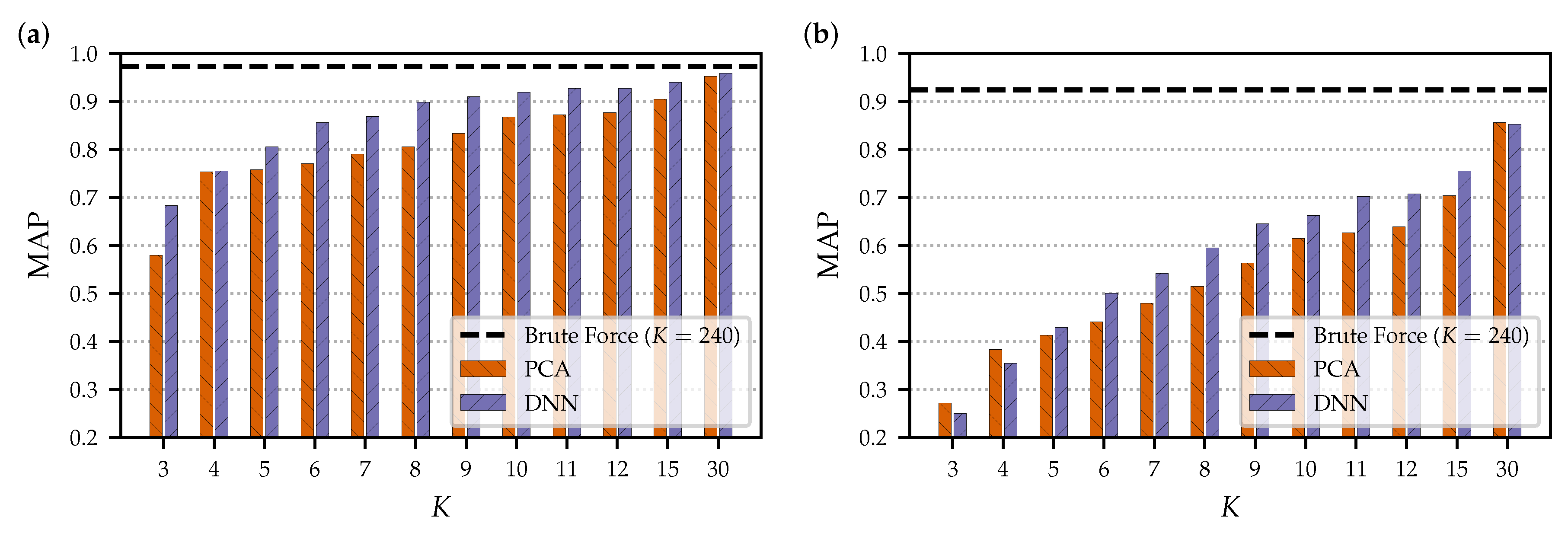
Figure 6 shows the MAP evaluation results for different embedding dimensionalities K on the smaller test set ${\mathbb{D}}_2$, as reported in the previous Section 5 (a) and on the extended data set ${\mathbb{D}}_3$ (b). As expected, we see a decrease in retrieval quality for the larger data set. The results for the brute-force approach decrease from an MAP of 0.996 for ${\mathbb{D}}_2$ to 0.924 for ${\mathbb{D}}_3$. The results based on the embedding approaches decrease even more. In particular, the smaller dimensionalities result in an MAP of less than 0.6; e.g., for $K=6$, the MAP is 0.441 and 0.500 for PCA and DNN, respectively. This confirms our assumption that the extended data set constitutes a harder task and leads to an increased probability for false negatives. One reason for the increased difficulty of the task is that there is a higher potential for confusion between the documents due to the increased data set size. Another reason is the increased diversity of database documents.

To gain more insights into these results, we now analyze the evaluation for each of the individual composers of the data set. In the following, we fix the dimensionality of $K=12$ as a typical example that gives a good trade-off between retrieval quality and speed, as shown in the previous experiments.

Table 8. Composer-wise evaluation results using the extended data set ${\mathbb{D}}_3$.

	Queries		Brute Force				PCA ($\mathit{K}=12$)				DNN ($\mathit{K}=12$)
			P@1	P${}_{\mathit{R}}$	MAP		P@1	P${}_{\mathit{R}}$	MAP		P@1	P${}_{\mathit{R}}$	MAP
Beethoven	160		0.963	0.827	0.879		0.631	0.456	0.521		0.669	0.477	0.538
Chopin	2930		0.996	0.876	0.932		0.899	0.626	0.686		0.936	0.765	0.825
Vivaldi	210		0.967	0.921	0.953		0.790	0.645	0.716		0.819	0.646	0.728
Brahms	240		0.992	0.960	0.976		0.754	0.543	0.619		0.796	0.593	0.667
Mahler	200		0.950	0.920	0.940		0.845	0.682	0.755		0.700	0.539	0.617
Mozart	200		1.000	0.864	0.907		0.630	0.390	0.443		0.560	0.349	0.399
Mussorgsky	660		0.967	0.834	0.877		0.718	0.482	0.545		0.642	0.452	0.516
Schumann	150		0.980	0.893	0.918		0.553	0.400	0.462		0.653	0.472	0.553
Tchaikovsky	420		0.983	0.892	0.925		0.729	0.493	0.566		0.621	0.492	0.543
Wagner	180		0.983	0.849	0.912		0.761	0.625	0.676		0.722	0.584	0.636
⌀ over queries			0.987	0.877	0.924		0.818	0.577	0.639		0.818	0.646	0.708

shows the detailed evaluation results for $K=12$. The rows correspond to the composers of the data set, and the last row reports the averaged evaluation measures over all queries and all composers. Note that composers with many queries have a stronger impact on this average compared to composers with few queries. The queries from the Chopin recordings result in an MAP value of 0.932 with the brute-force approach, 0.686 with PCA, and 0.825 with DNN. These numbers are lower than the ones we obtained for the smaller test set (0.972 for brute-force, 0.877 for PCA, and 0.928 for DNN; see Table 5). In particular, PCA suffers from using the larger test data set. The moderate loss for the DNN approach could point towards overfitting, because Chopin is also the most prominent composer of the training set. The queries from the Mahler recordings result in an MAP value of 0.940 with the brute-force approach, 0.755 with PCA, and 0.617 with DNN. Here, the DNN is considerably worse than the linear PCA-based projection. The late-romantic style of Mahler could be too different from the styles of the training set. The queries from the Schumann recordings result in an MAP value of 0.918 with the brute-force approach, 0.462 with PCA, and 0.553 with DNN. In this case, the DNN achieves better results than those of the PCA. Note that Schumann is not part of the training set and that the respective work is a piano concerto, which is a classical music genre that is also not covered in the training set.

A possible explanation for the poorer results of the embedding methods could be that the embeddings are just overfitted to the composers and styles of the training set and are not very discriminative in general. In the next section, we will question this argument by considering longer query audio fragments.

6.3. Dependency on Query Length

A possible explanation for the results of the previous section is that the query length of 20 s is not discriminative enough to identify all versions of the same piece. To analyze this hypothesis, we increased the query length in the following experiments. An obvious way to do this is to increase the query shingle length. However, we want to keep our shingle size fixed to keep the same database structure for different query lengths. Therefore, instead of increasing the query shingle length, we used multiple successive shingles for each query.

Recall that, in our previous approach (see Section 3), we compared a query ($\mathrm{Q}$) and a document ($\mathrm{D}$) by performing a nearest neighbor search of a single query shingle ${\mathit{S}}^{\mathrm{Q}}$ and all shingles from the set ${\mathbb{S}}^{\mathrm{D}}$ of document submatrices (see Equation (2)). The squared Euclidean distance to the nearest neighbor ${\delta }_{\mathrm{D}}({\mathit{S}}^{\mathrm{Q}})\in {\mathbb{R}}_{\ge 0}$ is regarded as the document-wise distance between $\mathrm{Q}$ and $\mathrm{D}$ and was used for ranking all documents of the database. Here, instead of a single query shingle ${\mathit{S}}^{\mathrm{Q}}$, we collected a set of successive shingles ${\mathbb{S}}^{\mathrm{Q}}$ from the query recording, as done for the documents (see Equation (2)). Instead of using a hop size $H=1$ (as for the documents), we used a hop size of $H=L/2=10$. Denoting the number of shingles per query by $\lambda :=|{\mathbb{S}}^{\mathrm{Q}}|$, a query covers $(\lambda -1)\times 10+20$ s of audio content. For each of these shingles, we computed the document-wise distance ${\delta }_{\mathrm{D}}$, as done previously (see Equation (6)). To obtain a single distance value between the query and the database document, the resulting shingle-wise distances were simply averaged:

$$\overline{{\delta }_{\mathrm{D}}}({\mathbb{S}}^{\mathrm{Q}})=\frac{1}{\lambda }\sum _{\mathit{S}\in {\mathbb{S}}^{\mathrm{Q}}}{\delta }_{\mathrm{D}}(\mathit{S}).$$

(10)

Finally, all database documents $\mathrm{D}\in \mathbb{D}$ were ranked by their averaged distances $\overline{{\delta }_{\mathrm{D}}}({\mathbb{S}}^{\mathrm{Q}})\in {\mathbb{R}}_{\ge 0}$ in ascending order. Note that our previous experiments are the special case of $\lambda =1$ (query length: 20 s).

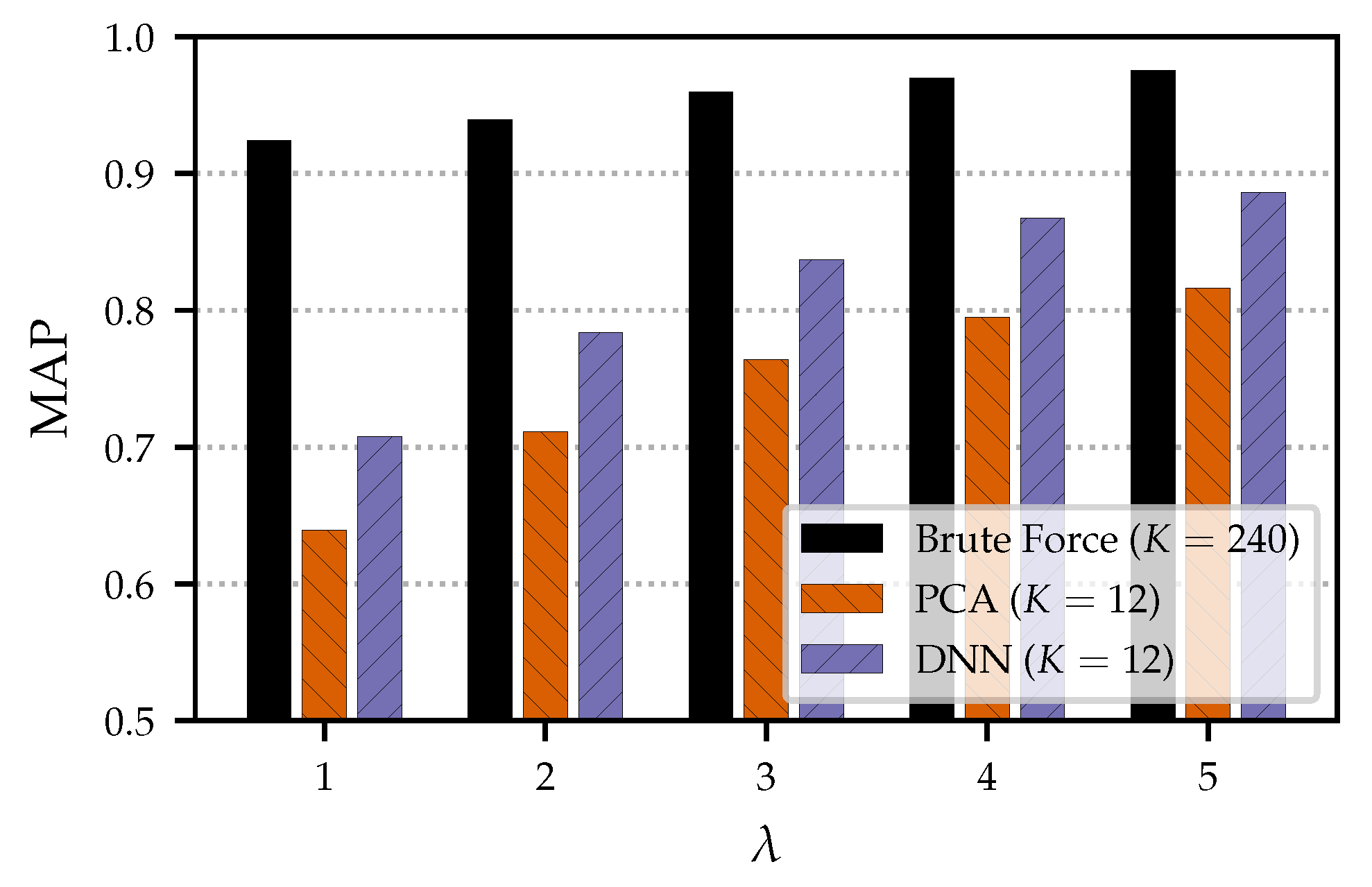
For our experiments, we sampled 10 queries from each recording in an equidistant way, as before. Note each query now consists of multiple shingles. Figure 7 shows the MAP evaluation results for $K=12$ using different query lengths on the extended data set. The retrieval quality considerably improves with increasing query length, e.g., the brute-force approach improves from an MAP value of 0.924 for $\lambda =1$ to 0.976 for $\lambda =5$. Similarly, the MAP values for the PCA- and DNN-based approaches increase strongly with the query length.

Table 9. Composer-wise evaluation results using the extended data set ${\mathbb{D}}_3$ for $\lambda =5$ (query length: 60 s).

	Queries		Brute Force				PCA ($\mathit{K}=12$)				DNN ($\mathit{K}=12$)
			P@1	P${}_{\mathit{R}}$	MAP		P@1	P${}_{\mathit{R}}$	MAP		P@1	P${}_{\mathit{R}}$	MAP
Beethoven	160		0.956	0.921	0.941		0.800	0.598	0.666		0.838	0.633	0.698
Chopin	2930		0.997	0.943	0.974		0.973	0.727	0.813		0.979	0.886	0.937
Vivaldi	210		1.000	0.986	0.996		0.971	0.864	0.918		0.976	0.864	0.925
Brahms	240		1.000	0.998	0.999		0.996	0.912	0.950		0.992	0.943	0.967
Mahler	200		0.985	0.976	0.982		0.960	0.900	0.935		0.935	0.846	0.891
Mozart	200		1.000	0.966	0.980		0.935	0.639	0.704		0.880	0.600	0.670
Mussorgsky	660		0.992	0.937	0.960		0.933	0.703	0.773		0.865	0.697	0.756
Schumann	150		0.993	0.977	0.983		0.800	0.630	0.681		0.920	0.780	0.840
Tchaikovsky	420		0.998	0.984	0.990		0.952	0.776	0.839		0.929	0.788	0.838
Wagner	180		1.000	0.956	0.975		0.978	0.884	0.922		0.989	0.904	0.940
⌀ over queries			0.995	0.953	0.976		0.956	0.744	0.816		0.951	0.835	0.886

shows the results for each of the composers of the data set for $\lambda =5$ (query length: 60 s). For Chopin, the DNN (MAP: 0.937) outperforms PCA (MAP: 0.813) and comes close to brute force (MAP: 0.974). For Mahler, PCA (MAP: 0.935) is slightly better than the DNN (MAP: 0.891). For Schumann’s piano concerto, the DNN (MAP: 0.840) substantially outperforms PCA (MAP: 0.681). In contrast to the Chopin results, this cannot be explained by overfitting, because neither Schumann nor any piano concerto was part of the training set. Furthermore, we achieved an MAP value of 0.967 for the pieces by Brahms using the DNN approach. This is the best result among all composers for this approach, even better than for the composers of the training set. This shows a certain generalizability of the DNN embedding method.

In summary, our experiments show that low-dimensional embeddings need a longer query length to be discriminative enough when using a larger data set. Note that a query length of 60 s is still a medium duration compared to studies for related tasks. For example, in popular music cover song retrieval, an entire recording is often used as a query—e.g., in the approach by Serrà et al. [24] or the work by Casey et al. [9] (using entire recordings as queries, though with a short shingle length of 3 s). Furthermore, we showed that, in general, composers outside the training set do not necessarily lead to worse retrieval results compared to composers contained in the training set. Thus, we can assume a certain generalizability of our approach within the common practice period of Western classical music.

6.4. Distance Analysis

In the previous section, we addressed issues of scalability and generalizability in relation to the query length. Now we want to gain further insights into the challenges that occur in the retrieval scenario. For example, beyond rank-based evaluation measures, we want to find out whether particular compositions are easier or harder for retrieval than others, e.g., due to harmonic or melodic characteristics. Recall from Section 3 that the ranks are computed on the basis of the distances that appear between queries and documents. The retrieval problem is well behaved if the distances between queries and documents of the same piece of music (relevant documents) are substantially smaller than the distances between queries and documents of different pieces (non-relevant documents). To understand how well behaved our problem is, we now analyze the distances that appear in the nearest neighbor search.

Recall that we have $R\in \mathbb{N}$ relevant documents for a given query. We want to compare the distances to the relevant documents with the distances to the non-relevant documents. Since most of the non-relevant documents should be easily distinguishable from the relevant ones, we restrict our analysis to the most difficult non-relevant documents for the task. To balance the numbers of relevant and non-relevant documents, we only consider the R non-relevant documents with the smallest distances to the given query. Small distances mean that these non-relevant documents have the greatest confusion potential with the relevant documents. In the following, we analyze the relation of the distributions of distances for relevant documents and non-relevant documents, respectively. The relation between these distributions indicates how difficult the retrieval problem is. However, the analysis of the relation between the distributions has to be taken with care, because versions with different difficulties are included in a single distribution. For that reason, a strong separation of the distributions is a sufficient condition for perfect retrieval results, but not a necessary condition. In other words, even if the overlap between the distributions is large, the retrieval may still give excellent results. In this sense, we regard the distributions only as weak indicators and only evaluate them by visual inspection in the following. For a more statistically rigorous analysis of such distributions, we refer to the study by Casey et al. [9].

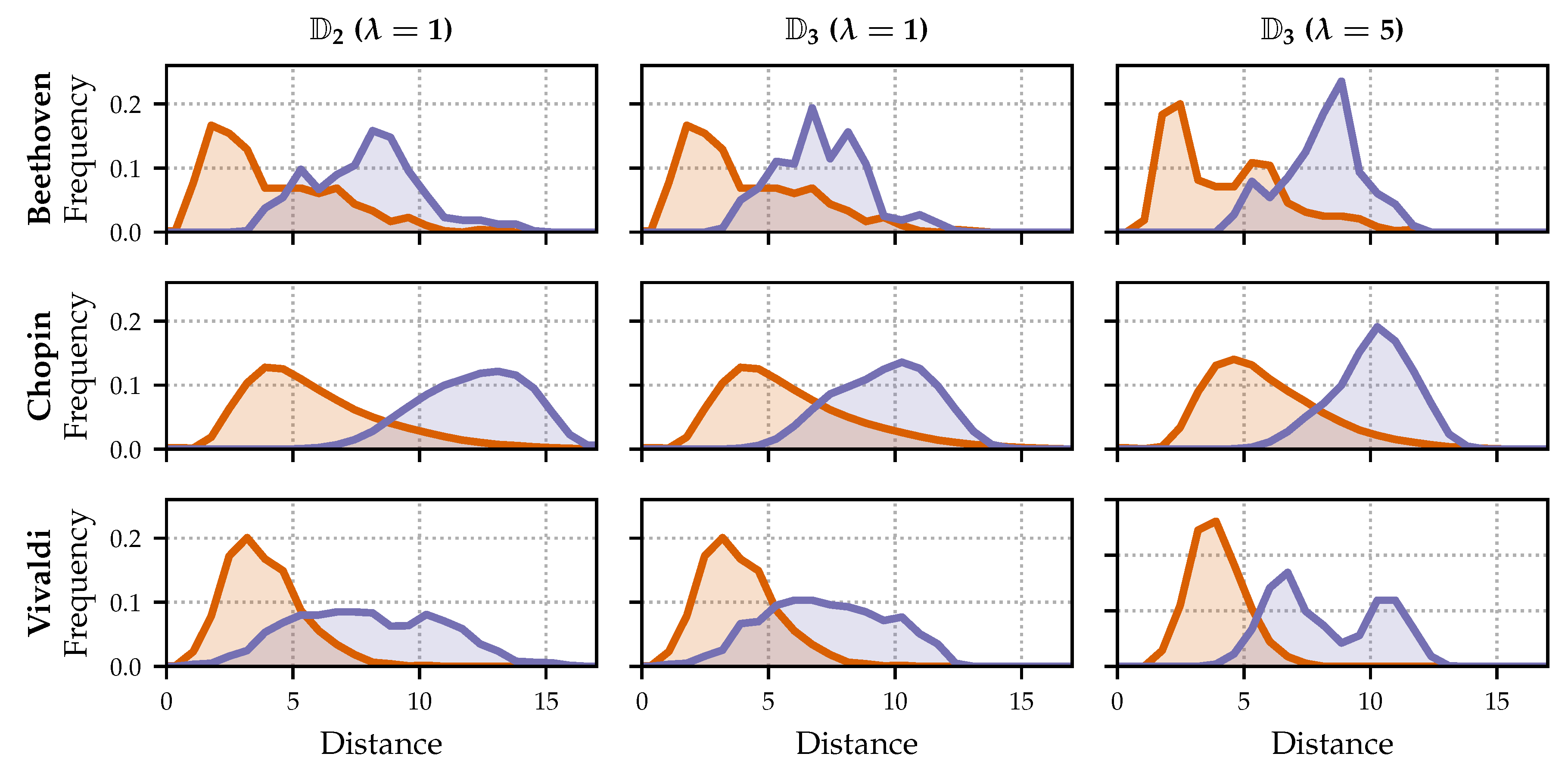
Figure 8 shows such distributions for the brute-force approach, where the distributions of relevant document distances appear in orange color and the distributions of non-relevant document distances appear in blue color. The three rows show distributions for the composers that are part of both ${\mathbb{D}}_2$ and ${\mathbb{D}}_3$ (Beethoven, Chopin, and Vivaldi); the three columns correspond to different evaluation settings. The left column refers to the smaller test set ${\mathbb{D}}_2$ with $\lambda =1$ (query length: 20 s), the middle column refers to the extended test set ${\mathbb{D}}_3$ with $\lambda =1$ (query length: 20 s), and the right column refers to the extended test set ${\mathbb{D}}_3$ with $\lambda =5$ (query length: 60 s). Considering Chopin in the left column, we see that the center of the orange distribution is much further to the left than the blue distribution. This means that the distances to the relevant documents are generally smaller than the distances to the non-relevant documents. We also see a small overlap between both distributions, which is caused by the fact that some distances to non-relevant documents are smaller than the greatest distances to relevant documents. However, since the distances that lead to the overlap could relate to different queries, we cannot conclude that this necessarily leads to confusion in the retrieval step. In general, since the overlap is small, the distributions indicate that the retrieval problem is well behaved for Chopin. For Beethoven and Vivaldi (left column), there is more overlap. This suggests that the Chopin pieces are “easier” in the sense that they are more discriminative than other pieces. For the extended data set (middle column), we see similar tendencies for all three composers. The blue distributions come a bit closer to the orange ones with respect to their relation for the smaller data set (left column). The orange distributions are identical to the ones for the smaller data set because the distances to the relevant documents are the same. Only the distances to non-relevant documents decrease, because the extended data set contains more non-relevant documents with possibly smaller distances. When using a longer query length ($\lambda =5$, right column), the orange and blue distributions are better separated for all three composers. The distances for the relevant documents only slightly increase because of the longer query length, but the distances to the non-relevant documents increase strongly, which leads to a better separation between the distributions.

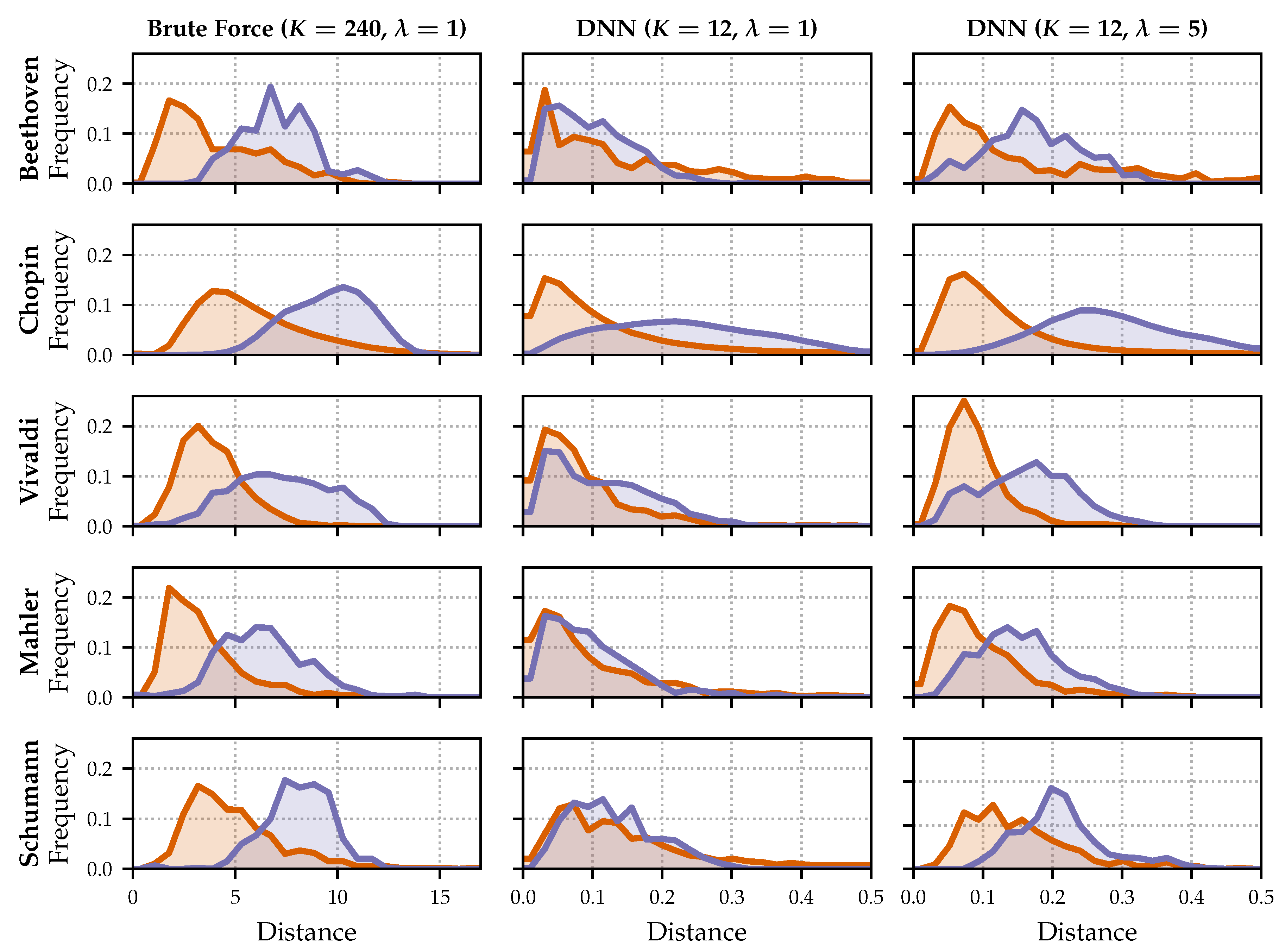
So far, we analyzed distributions for the brute-force approach to gain insights into the musical complexity of the retrieval task. In the following, we want to understand the effect of the embedding on the distributions. Figure 9 shows further distributions for the extended test set ${\mathbb{D}}_3$ and five selected composers (Beethoven, Chopin, Vivaldi, Mahler, and Schumann). The left column refers to the brute-force approach ($K=240$) with $\lambda =1$ (query length: 20 s), the middle column refers to the DNN embedding approach ($K=12$) with $\lambda =1$ (query length: 20 s), and the right column refers to the DNN embedding approach ($K=12$) with $\lambda =5$ (query length: 60 s). Note that the absolute distances between the different approaches are not comparable, but the relations between orange and blue distributions are meaningful. The distance measure is always the squared Euclidean distance, cf. Equation (5). However, for the brute-force approach, we have sequences of 20 non-negative ${\ell }^2$-normalized vectors of size 12, which are then flattened (distance range $[0,40]$). For the DNN approach, we have real-valued ${\ell }^2$-normalized vectors of size 12 (distance range $[0,4]$).

For the brute-force approach (left column), the new composers of the extended data set (Mahler, Schumann) behave similarly to the previous ones. The middle column reflects the weaker results for the low-dimensional embeddings with a shorter query length. As expected, there are strong overlaps between the orange and blue distributions. We can also see that there are some distances close to zero in the orange distributions. This can be explained by the neural network training, where the anchor and positive embeddings are pushed close together. However, the anchor and negative embeddings do not seem to be pulled apart the same way. For Chopin, the most prominent composer of the training set ${\mathbb{D}}_1$, the separation between the distributions is clearer. When using longer queries ($\lambda =5$, right column), all orange and blue distributions are better separated. This holds for Chopin, where the initial situation ($\lambda =1$) is better, as well as for composers with heavily overlapping distributions for $\lambda =1$—e.g., Schumann.

7. Conclusions

In this paper, we proposed two dimensionality reduction methods for learning compact embeddings of audio shingles (short sequences of chroma vectors) for a cross-version retrieval scenario in the context of Western classical music. We showed that our strategy of reducing entire shingles results in better retrieval quality and faster speed compared to those of the previous approach of reducing individual chroma vectors [12]. In our experiments, we greatly reduced the dimensionality of shingles—from 240 to below 12—with only little loss in retrieval quality. Both PCA and neural networks with triplet loss turned out to be effective for this task. In particular, we found that neural networks are beneficial for small dimensionalities of between 6 and 12. Such small dimensions allow for indexing by simple nearest neighbor trees, which could be the foundation of fast content-based audio retrieval in large classical music databases where efficiency is an important issue. We also showed that the database size has a strong impact on the retrieval results, especially when using dimensionality reduction methods. Applying such techniques, one needs a longer query length to be discriminative enough on a larger data set. Increasing the query length from 20 to 60 s results in a high retrieval accuracy, even for low-dimensional embeddings. We also showed that our approaches generalize to composers of the common practice period of Western classical music which are not contained in the training set. Furthermore, we analyzed the distances that appear in the nearest neighbor search to gain insights into the challenges of the retrieval scenario. For example, we showed that the distance distributions for different composers can differ strongly and give the indication that certain composers or pieces are more difficult for retrieval than others. In future work, we will investigate whether training on larger data sets can make the embeddings more robust for shorter query lengths. Furthermore, up to now, we used CENS features—which are state-of-the-art for the given task—as the input. We want to investigate if good embeddings can be learned from less specialized input features such as “raw” chroma features, spectrograms, or even waveforms.