


Using Mid-Infrared Spectroscopy to Optimize Throughput and Costs of Soil Organic Carbon and Nitrogen Estimates: An Assessment in Grassland Soils


Abstract
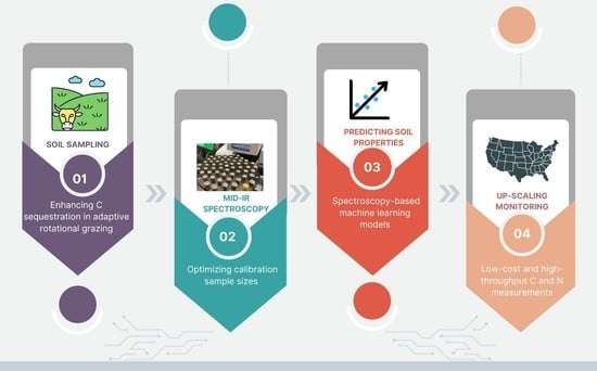
1. Introduction
2. Materials and Methods
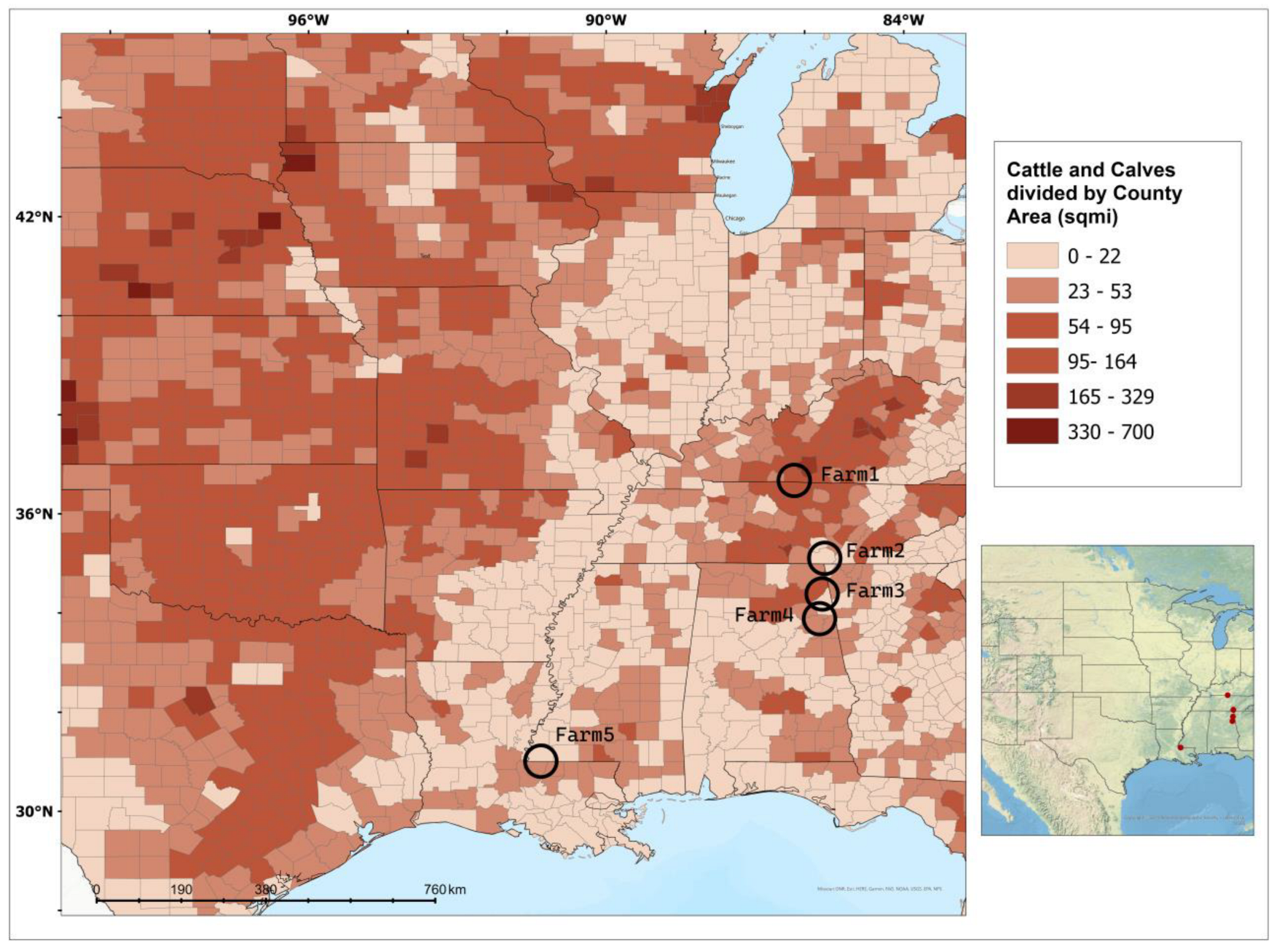
2.1. Study Sites and Soil Sampling
2.2. Soil Analysis
2.3. MIR Measurements
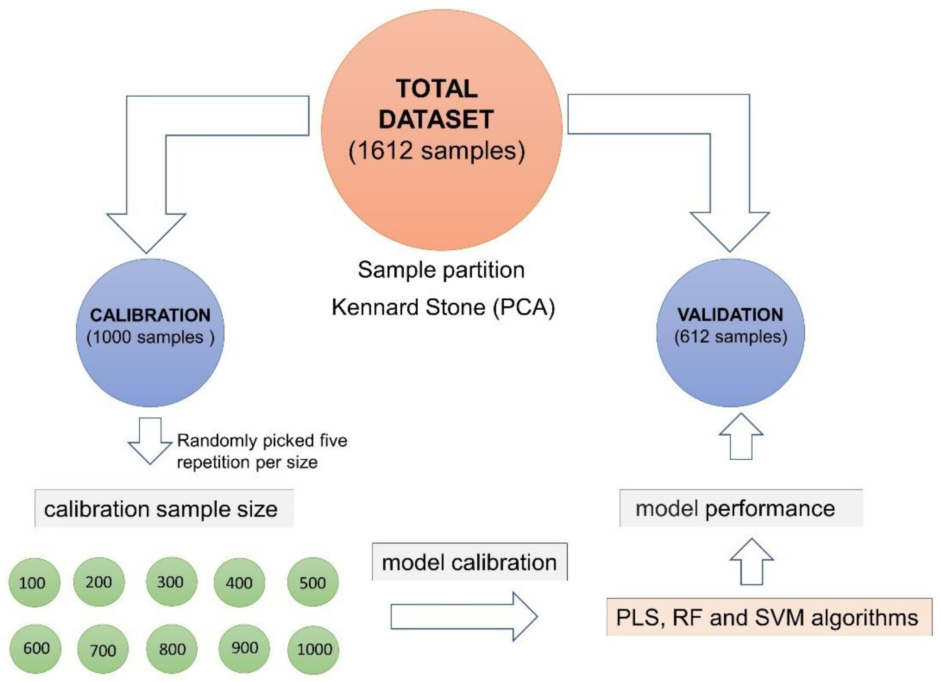
2.4. Sample Selection
2.5. Model Calibration
2.6. Model Validation
3. Results
3.1. Descriptive Analysis of Soil Data
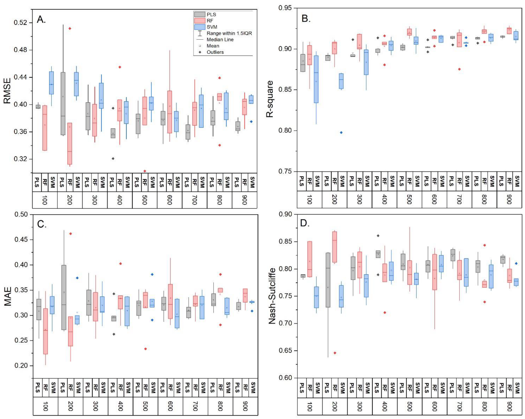
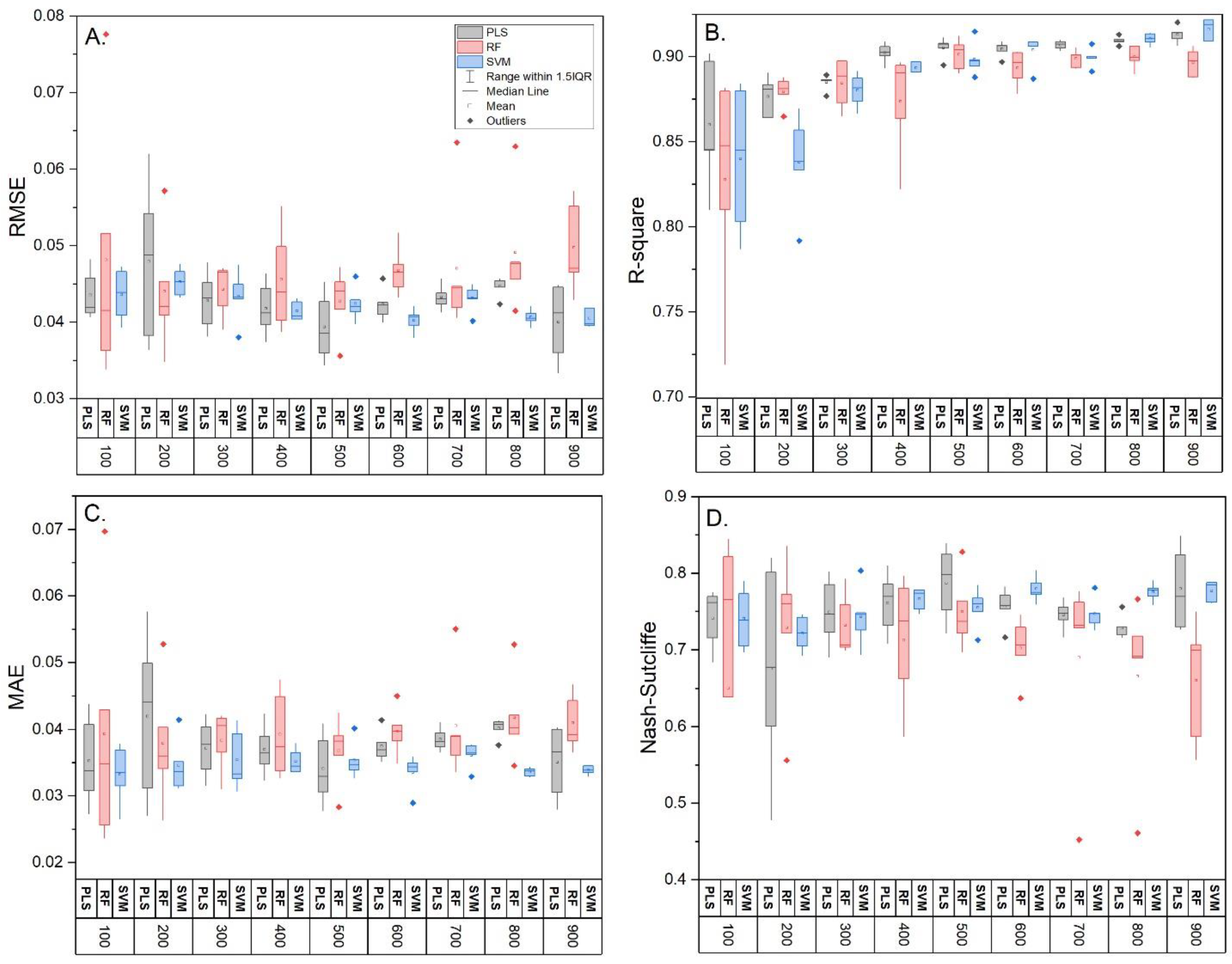
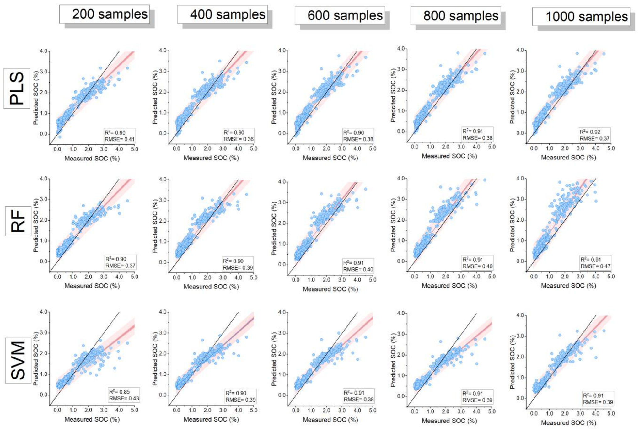
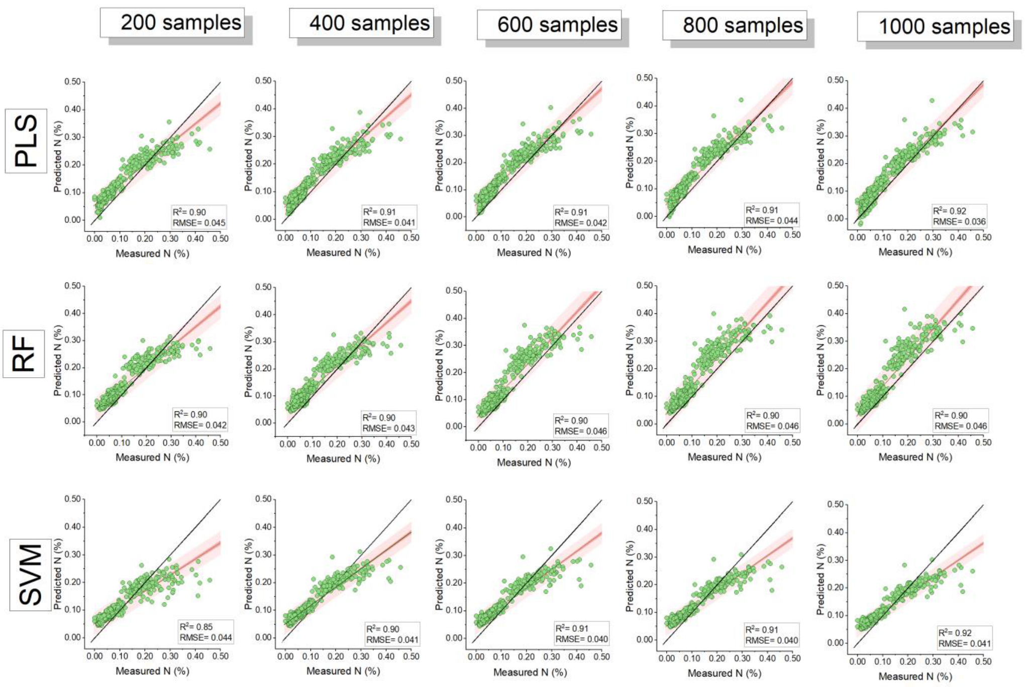
3.2. Model Comparison and Influence of Training Sample Size
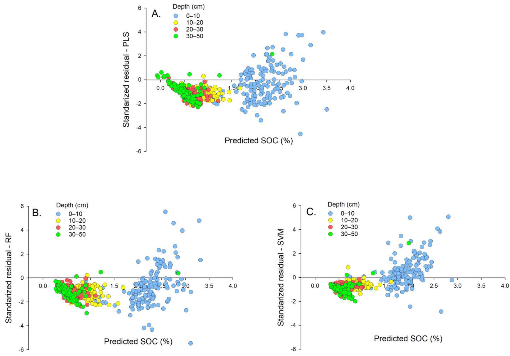
3.3. Influence of Sampling Depth and Farm Site on Model Accuracy
3.4. Cost Analysis
4. Discussion
5. Conclusions
Supplementary Materials
Author Contributions
Funding
Data Availability Statement
Conflicts of Interest
References
- Sanderman, J.; Savage, K.; Dangal, S.R.S. Mid-Infrared Spectroscopy for Prediction of Soil Health Indicators in the United States. Soil Sci. Soc. Am. J. 2020, 84, 251–261. [Google Scholar] [CrossRef]
- Seybold, C.A.; Ferguson, R.; Wysocki, D.; Bailey, S.; Anderson, J.; Nester, B.; Schoeneberger, P.; Wills, S.; Libohova, Z.; Hoover, D.; et al. Application of Mid-Infrared Spectroscopy in Soil Survey. Soil Sci. Soc. Am. J. 2019, 83, 1746–1759. [Google Scholar] [CrossRef]
- Cotrufo, M.F.; Ranalli, M.G.; Haddix, M.L.; Six, J.; Lugato, E. Soil Carbon Storage Informed by Particulate and Mineral-Associated Organic Matter. Nat. Geosci. 2019, 12, 989–994. [Google Scholar] [CrossRef]
- Keller, A.B.; Borer, E.T.; Collins, S.L.; DeLancey, L.C.; Fay, P.A.; Hofmockel, K.S.; Leakey, A.D.B.; Mayes, M.A.; Seabloom, E.W.; Walter, C.A.; et al. Soil Carbon Stocks in Temperate Grasslands Differ Strongly across Sites but Are Insensitive to Decade-Long Fertilization. Glob. Chang. Biol. 2022, 28, 1659–1677. [Google Scholar] [CrossRef] [PubMed]
- Rocci, K.S.; Barker, K.S.; Seabloom, E.W.; Borer, E.T.; Hobbie, S.E.; Bakker, J.D.; MacDougall, A.S.; McCulley, R.L.; Moore, J.L.; Raynaud, X.; et al. Impacts of Nutrient Addition on Soil Carbon and Nitrogen Stoichiometry and Stability in Globally-Distributed Grasslands. Biogeochemistry 2022, 159, 353–370. [Google Scholar] [CrossRef]
- Reinermann, S.; Asam, S.; Kuenzer, C. Remote Sensing of Grassland Production and Management—A Review. Remote Sens. 2020, 12, 1949. [Google Scholar] [CrossRef]
- Jones, M.O.; Naugle, D.E.; Twidwell, D.; Uden, D.R.; Maestas, J.D.; Allred, B.W. Beyond Inventories: Emergence of a New Era in Rangeland Monitoring. Rangel. Ecol. Manag. 2020, 73, 577–583. [Google Scholar] [CrossRef]
- Asner, G.P.; Wessman, C.A.; Bateson, C.A.; Privette, J.L. Impact of Tissue, Canopy, and Landscape Factors on the Hyperspectral Reflectance Variability of Arid Ecosystems. Remote Sens. Environ. 2000, 74, 69–84. [Google Scholar] [CrossRef]
- Angelopoulou, T.; Tziolas, N.; Balafoutis, A.; Zalidis, G.; Bochtis, D. Remote Sensing Techniques for Soil Organic Carbon Estimation: A Review. Remote Sens. 2019, 11, 676. [Google Scholar] [CrossRef]
- Chabrillat, S.; Ben-Dor, E.; Cierniewski, J.; Gomez, C.; Schmid, T.; van Wesemael, B. Imaging Spectroscopy for Soil Mapping and Monitoring. Surv. Geophys. 2019, 40, 361–399. [Google Scholar] [CrossRef]
- Stanley, P.L.; Rowntree, J.E.; Beede, D.K.; DeLonge, M.S.; Hamm, M.W. Impacts of Soil Carbon Sequestration on Life Cycle Greenhouse Gas Emissions in Midwestern USA Beef Finishing Systems. Agric. Syst. 2018, 162, 249–258. [Google Scholar] [CrossRef]
- Mosier, S.; Apfelbaum, S.; Byck, P.; Calderon, F.; Teague, R.; Thompson, R.; Cotrufo, M.F. Adaptive Multi-Paddock Grazing Enhances Soil Carbon and Nitrogen Stocks and Stabilization through Mineral Association in Southeastern U.S. Grazing Lands. J. Environ. Manag. 2021, 288, 112409. [Google Scholar] [CrossRef]
- Ng, W.; Minasny, B.; Malone, B.; Filippi, P. In Search of an Optimum Sampling Algorithm for Prediction of Soil Properties from Infrared Spectra. PeerJ 2018, 2018, e5722. [Google Scholar] [CrossRef]
- Zhang, Y.; Saurette, D.D.; Easher, T.H.; Ji, W.; Adamchuck, V.I.; Biswas, A. Comparison of Sampling Designs for Calibrating Digital Soil Maps at Multiple Depths. Pedosphere 2022, 32, 588–601. [Google Scholar] [CrossRef]
- Araújo, S.R.; Wetterlind, J.; Demattê, J.A.M.; Stenberg, B. Improving the Prediction Performance of a Large Tropical Vis-NIR Spectroscopic Soil Library from Brazil by Clustering into Smaller Subsets or Use of Data Mining Calibration Techniques. Eur. J. Soil Sci. 2014, 65, 718–729. [Google Scholar] [CrossRef]
- Wold, S.; Sjöström, M.; Eriksson, L. PLS-Regression: A Basic Tool of Chemometrics. Chemom. Intell. Lab. Syst. 2001, 58, 109–130. [Google Scholar] [CrossRef]
- Deiss, L.; Margenot, A.J.; Culman, S.W.; Demyan, M.S. Tuning Support Vector Machines Regression Models Improves Prediction Accuracy of Soil Properties in MIR Spectroscopy. Geoderma 2020, 365, 114227. [Google Scholar] [CrossRef]
- Lucà, F.; Conforti, M.; Castrignanò, A.; Matteucci, G.; Buttafuoco, G. Effect of Calibration Set Size on Prediction at Local Scale of Soil Carbon by Vis-NIR Spectroscopy. Geoderma 2017, 288, 175–183. [Google Scholar] [CrossRef]
- Anderson, S.T. Economics, Helium, and the U.S. Federal Helium Reserve: Summary and Outlook. Nat. Resour. Res. 2018, 27, 455–477. [Google Scholar] [CrossRef]
- VM0021 Soil Carbon Quantification Methodology, v1.0-Verra. Available online: https://verra.org/methodology/vm0021-soil-carbon-quantification-methodology-v1-0/ (accessed on 18 October 2022).
- Sherrod, L.A.; Dunn, G.; Peterson, G.A.; Kolberg, R.L. Inorganic Carbon Analysis by Modified Pressure-Calcimeter Method. Soil Sci. Soc. Am. J. 2002, 66, 299–305. [Google Scholar] [CrossRef]
- Leuthold, S.J.; Haddix, M.L.; Lavallee, J.; Cotrufo, M.F. Physical Fractionation Techniques. Ref. Modul. Earth Syst. Environ. Sci. 2022. [Google Scholar] [CrossRef]
- Kennard, R.W.; Stone, L.A. Computer Aided Design of Experiments. Technometrics 1969, 11, 137–148. [Google Scholar] [CrossRef]
- Wickham, H.; François, R.; Henry, L.; Müller, K. Dplyr: A Grammar of Data Manipulation. 2022. Available online: https://dplyr.tidyverse.org (accessed on 25 October 2022).
- Kuhn, M. Building Predictive Models in R Using the Caret Package. J. Stat. Softw. 2008, 28, 1–26. [Google Scholar] [CrossRef]
- Pirouz, D.M. An Overview of Partial Least Squares. SSRN Electron. J. 2006. [CrossRef]
- Vapnik, V. The Support Vector Method of Function Estimation. In Nonlinear Modeling; Springer: Boston, MA, USA, 1998; pp. 55–85. [Google Scholar] [CrossRef]
- Breiman, L. Random Forests. Mach. Learn. 2001, 45, 5–32. [Google Scholar] [CrossRef]
- Ballabio, D.; Todeschini, R.; Todeschini, R.O.; Bahmani, A.; Consonni, V. Evaluation of model predictive ability by external validation techniques. J. Chemom. 2010, 24, 194–201. [Google Scholar] [CrossRef]
- Chai, T.; Draxler, R.R. Root Mean Square Error (RMSE) or Mean Absolute Error (MAE)? -Arguments against Avoiding RMSE in the Literature. Geosci. Model Dev. 2014, 7, 1247–1250. [Google Scholar] [CrossRef]
- Willmott, C.J.; Matsuura, K. Advantages of the Mean Absolute Error (MAE) over the Root Mean Square Error (RMSE) in Assessing Average Model Performance. Clim. Res. 2005, 30, 79–82. [Google Scholar] [CrossRef]
- Jierula, A.; Wang, S.; Oh, T.M.; Wang, P. Study on Accuracy Metrics for Evaluating the Predictions of Damage Locations in Deep Piles Using Artificial Neural Networks with Acoustic Emission Data. Appl. Sci. 2021, 11, 2314. [Google Scholar] [CrossRef]
- Ahmed, M.; Ahmad, S.; Ali Raza, M.; Kumar, U.; Ansar, M.; Abbas Shah, G.; Parsons, D.; Hoogenboom, G.; Palosuo, T.; Seidel, S.; et al. Models Calibration and Evaluation. In Systems Modeling; Springer: Singapore, 2020; pp. 151–178. [Google Scholar] [CrossRef]
- Anscombe, F.J.; Tukey, J.W. The Examination and Analysis of Residuals. Technometrics 1963, 5, 141–160. [Google Scholar] [CrossRef]
- Ng, W.; Minasny, B.; de Sousa Mendes, W.; Melo Demattê, J.A. The Influence of Training Sample Size on the Accuracy of Deep Learning Models for the Prediction of Soil Properties with Near-Infrared Spectroscopy Data. SOIL 2020, 6, 565–578. [Google Scholar] [CrossRef]
- Ramirez-Lopez, L.; Schmidt, K.; Behrens, T.; van Wesemael, B.; Demattê, J.A.M.; Scholten, T. Sampling Optimal Calibration Sets in Soil Infrared Spectroscopy. Geoderma 2014, 226, 140–150. [Google Scholar] [CrossRef]
- Rossel, R.A.V.; Behrens, T. Using Data Mining to Model and Interpret Soil Diffuse Reflectance Spectra. Geoderma 2010, 158, 46–54. [Google Scholar] [CrossRef]
- Tange, R.I.; Rasmussen, M.A.; Taira, E.; Bro, R. Benchmarking Support Vector Regression against Partial Least Squares Regression and Artificial Neural Network: Effect of Sample Size on Model Performance. J. Near Infrared Spectrosc. 2017, 25, 381–390. [Google Scholar] [CrossRef]
- Janik, L.J.; Merry, R.H.; Forrester, S.T.; Lanyon, D.M.; Rawson, A. Rapid Prediction of Soil Water Retention Using Mid Infrared Spectroscopy. Soil Sci. Soc. Am. J. 2007, 71, 507–514. [Google Scholar] [CrossRef]
- Ramírez, P.B.; Calderón, F.J.; Haddix, M.; Lugato, E.; Cotrufo, M.F. Using Diffuse Reflectance Spectroscopy as a High Throughput Method for Quantifying Soil C and N and Their Distribution in Particulate and Mineral-Associated Organic Matter Fractions. Front. Environ. Sci. 2021, 9, 153. [Google Scholar] [CrossRef]
- Baldock, J.A.; Beare, M.H.; Curtin, D.; Hawke, B. Stocks, Composition and Vulnerability to Loss of Soil Organic Carbon Predicted Using Mid-Infrared Spectroscopy. Soil Res. 2018, 56, 468–480. [Google Scholar] [CrossRef]
- Janik, L.J.; Skjemstad, J.O.; Shepherd, K.D.; Spouncer, L.R. The Prediction of Soil Carbon Fractions Using Mid-Infrared-Partial Least Square Analysis. Aust. J. Soil Res. 2007, 45, 73–81. [Google Scholar] [CrossRef]
- Li, S.; Viscarra Rossel, R.A.; Webster, R.; Raphael Viscarra Rossel, C.A. The Cost-Effectiveness of Reflectance Spectroscopy for Estimating Soil Organic Carbon. Eur. J. Soil Sci. 2021, 73, e13202. [Google Scholar] [CrossRef]
- Bellon-Maurel, V.; McBratney, A. Near-Infrared (NIR) and Mid-Infrared (MIR) Spectroscopic Techniques for Assessing the Amount of Carbon Stock in Soils-Critical Review and Research Perspectives. Soil Biol. Biochem. 2011, 43, 1398–1410. [Google Scholar] [CrossRef]


| Location | MAT (°C) | MAP (mm) | Grazing Practice | Year | n | Depth (cm) | SOC (%) | N (%) | BD (g/cm3) | |
|---|---|---|---|---|---|---|---|---|---|---|
| Farm 1 | AMP | 13 | 40 | 0–20 | 1.38 ± 0.83 | 0.16 ± 0.09 | 1.11 ± 0.20 | |||
| 17 | 20–30 | 0.29 ± 0.08 | 0.04 ± 0.01 | 1.22 ± 0.11 | ||||||
| Adolphus, | 13.8 | 1316 | 20 | 30–50 | 0.24 ± 0.07 | 0.05 ± 0.01 | 1.12 ± 0.15 | |||
| Kentucky | CG | 6 | 91 | 0–20 | 1.40 ± 0.87 | 0.16 ± 0.09 | 1.14 ± 0.14 | |||
| 43 | 20–30 | 0.29 ± 0.09 | 0.04 ± 0.01 | 1.10 ± 0.26 | ||||||
| 29 | 30–50 | 0.18 ± 0.04 | 0.04 ± 0.01 | 1.15 ± 0.12 | ||||||
| Farm 2 | AMP | 12 | 96 | 0–20 | 1.51 ± 0.96 | 0.17 ± 0.09 | 1.34 ± 0.12 | |||
| 37 | 20–30 | 0.47 ± 0.33 | 0.07 ± 0.02 | 1.45 ± 0.10 | ||||||
| Sequatchie, | 14.7 | 1432 | 44 | 30–50 | 0.29 ± 0.14 | 0.05 ± 0.01 | 1.53 ± 0.10 | |||
| Tennessee | CG | - | 91 | 0–20 | 1.28 ± 0.77 | 0.15 ± 0.08 | 1.41 ± 0.16 | |||
| 44 | 20–30 | 0.30 ± 0.14 | 0.05 ± 0.02 | 1.55 ± 0.10 | ||||||
| 44 | 30–50 | 0.26 ± 0.42 | 0.05 ± 0.04 | 1.61 ± 0.10 | ||||||
| Farm 3 | AMP | 29 | 91 | 0–20 | 1.28 ± 0.86 | 0.13 ± 0.09 | 1.45 ± 0.19 | |||
| 44 | 20–30 | 0.26 ± 0.08 | 0.03 ± 0.01 | 1.62 ± 0.1 | ||||||
| Fort Payne, | 15.1 | 1417 | 43 | 30–50 | 0.14 ± 0.04 | 0.02 ± 0 | 1.67 ± 0.05 | |||
| Alabama | CG | 17 | 78 | 0–20 | 1.03 ± 0.63 | 0.11 ± 0.06 | 1.52 ± 0.11 | |||
| 39 | 20–30 | 0.23 ± 0.08 | 0.03 ± 0.01 | 1.67 ± 0.12 | ||||||
| 33 | 30–50 | 0.13 ± 0.07 | 0.02 ± 0 | 1.74 ± 0.12 | ||||||
| Farm 4 | AMP | 24 | 92 | 0–20 | 1.35 ± 0.97 | 0.15 ± 0.10 | 1.4 ± 0.15 | |||
| 44 | 20–30 | 0.31 ± 0.16 | 0.04 ± 0.01 | 1.40 ± 0.10 | ||||||
| Piedmont, | 15.7 | 1352 | 36 | 30–50 | 0.18 ± 0.11 | 0.03 ± 0.01 | 1.47 ± 0.12 | |||
| Alabama | CG | - | 88 | 0–20 | 1.28 ± 0.75 | 0.12 ± 0.07 | 1.31 ± 0.21 | |||
| 40 | 20–30 | 0.34 ± 0.15 | 0.04 ± 0.01 | 1.45 ± 0.16 | ||||||
| 31 | 30–50 | 0.25 ± 0.26 | 0.03 ± 0.02 | 1.50 ± 0.19 | ||||||
| Farm 5 | AMP | 10 | 90 | 0–20 | 1.87 ± 1.36 | 0.21 ± 0.14 | 1.24 ± 0.19 | |||
| 45 | 20–30 | 0.3 ± 0.13 | 0.05 ± 0.01 | 1.44 ± 0.08 | ||||||
| Woodville, | 19 | 1649 | 45 | 30–50 | 0.15 ± 0.05 | 0.03 ± 0.01 | 1.41 ± 0.34 | |||
| Mississippi | CG | 38 | 89 | 0–20 | 1.46 ± 1.00 | 0.16 ± 0.10 | 1.22 ± 0.22 | |||
| 45 | 20–30 | 0.27 ± 0.08 | 0.05 ± 0.01 | 1.42 ± 0.09 | ||||||
| 43 | 30–50 | 0.15 ± 0.03 | 0.04 ± 0.01 | 1.47 ± 0.22 |
| Soil Organic Carbon (%) | Total Soil Nitrogen (%) | ||||||||
|---|---|---|---|---|---|---|---|---|---|
| Sample Size | Model | RMSE | R-Square | MAE | Nash– Sutcliffe | RMSE | R-Square | MAE | Nash–Sutcliffe |
| 100 (n = 5) | PLS | 0.40 ± 0 a | 0.89 ± 0.01 a | 0.31 ± 0.03 a | 0.79 ± 0 a | 0.044 ± 0.003 a | 0.86 ± 0.03 a | 0.035 ± 0.007 a | 0.74 ± 0.04 a |
| RF | 0.37 ± 0.03 a | 0.89 ± 0.02 a | 0.27 ± 0.05 a | 0.81 ± 0.03 a | 0.048 ± 0.018 a | 0.83 ± 0.06 a | 0.039 ± 0.019 a | 0.65 ± 0.25 a | |
| SVM | 0.43 ± 0.02 a | 0.86 ± 0.03 a | 0.32 ± 0.03 a | 0.75 ± 0.02 a | 0.044 ± 0.003 a | 0.84 ± 0.04 a | 0.033 ± 0.005 a | 0.74 ± 0.04 a | |
| 400 (n = 5) | PLS | 0.36 ± 0.02 b | 0.90 ± 0.01 a | 0.30 ± 0.03 a | 0.83 ± 0.02 b | 0.042 ± 0.004 a | 0.90 ± 0.01 b | 0.037 ± 0.004 a | 0.76 ± 0.04 a |
| RF | 0.39 ± 0.04 a | 0.90 ± 0.01 a | 0.33 ± 0.04 a | 0.79 ± 0.04 a | 0.046 ± 0.007 a | 0.87 ± 0.03 a | 0.039 ± 0.007 a | 0.71 ± 0.08 a | |
| SVM | 0.39 ± 0.02 b | 0.90 ± 0.01 b | 0.31 ± 0.03 a | 0.80 ± 0.02 b | 0.041 ± 0.001 a | 0.89 ± 0.00 b | 0.035 ± 0.002 a | 0.77 ± 0.01 a | |
| 1000 (n = 1) | PLS | 0.37 | 0.92 | 0.32 | 0.82 | 0.036 | 0.92 | 0.030 | 0.83 |
| RF | 0.47 | 0.90 | 0.37 | 0.70 | 0.046 | 0.90 | 0.038 | 0.71 | |
| SVM | 0.39 | 0.91 | 0.31 | 0.79 | 0.041 | 0.92 | 0.034 | 0.77 | |
| One-Time Cost (USD) | Yearly Cost (USD) | Data Acquisition Cost (USD) | Cost CN Analysis (USD) | |||||
|---|---|---|---|---|---|---|---|---|
| Sample Preparation | Technician | n = 400 | n = 1000 | |||||
| Method | Instrument (a) | Maintenance | Equipment | Lab. Supplies (<2 mm) (d) | Cost (Labor/h) (USD) | Time (Sample/h) | ||
| FT-IR Spectrometer | 50,000 | 3500 | 9000 (c) | 0.17 | 17.5 | 12.0 (e) | 768.0 | 1920.0 |
| Dry combustion analyzer (a) | 80,000 | 1700 (b) | N/A | 1.70 | 17.5 | 4.0 (f) | 2780.0 | 6950.0 |
Publisher’s Note: MDPI stays neutral with regard to jurisdictional claims in published maps and institutional affiliations. |
© 2022 by the authors. Licensee MDPI, Basel, Switzerland. This article is an open access article distributed under the terms and conditions of the Creative Commons Attribution (CC BY) license (https://creativecommons.org/licenses/by/4.0/).
Share and Cite
Ramírez, P.B.; Mosier, S.; Calderón, F.; Cotrufo, M.F. Using Mid-Infrared Spectroscopy to Optimize Throughput and Costs of Soil Organic Carbon and Nitrogen Estimates: An Assessment in Grassland Soils. Environments 2022, 9, 149. https://doi.org/10.3390/environments9120149
Ramírez PB, Mosier S, Calderón F, Cotrufo MF. Using Mid-Infrared Spectroscopy to Optimize Throughput and Costs of Soil Organic Carbon and Nitrogen Estimates: An Assessment in Grassland Soils. Environments. 2022; 9(12):149. https://doi.org/10.3390/environments9120149
Chicago/Turabian StyleRamírez, Paulina B., Samantha Mosier, Francisco Calderón, and M. Francesca Cotrufo. 2022. "Using Mid-Infrared Spectroscopy to Optimize Throughput and Costs of Soil Organic Carbon and Nitrogen Estimates: An Assessment in Grassland Soils" Environments 9, no. 12: 149. https://doi.org/10.3390/environments9120149
APA StyleRamírez, P. B., Mosier, S., Calderón, F., & Cotrufo, M. F. (2022). Using Mid-Infrared Spectroscopy to Optimize Throughput and Costs of Soil Organic Carbon and Nitrogen Estimates: An Assessment in Grassland Soils. Environments, 9(12), 149. https://doi.org/10.3390/environments9120149