Article

A New Testing Facility to Investigate the Removal Processes of Indoor Air Contaminants with Different Cleaning Technologies and to Better Assess and Exploit Their Performances

1
Istituto per i Sistemi Biologici del CNR, Area della Ricerca di Roma 1, Via Salaria Km 29,300, 00015 Rome, Italy
2
Istituto di Ricerca sugli Ecosistemi Terrestri (IRET-CNR), Area della Ricerca di Roma 1, Via Salaria Km 29,300, 00015 Rome, Italy
3
Istituto sull’Inquinamento Atmosferico del CNR, Area della Ricerca di Roma 1, Via Salaria Km 29,300, 00015 Rome, Italy
4
Istituto di Biologia e Biotecnologia Agraria del CNR, Area della Ricerca di Roma 1, Via Salaria Km 29,300, 00015 Rome, Italy
5
RI.EL.CO Ambiente S.r.l., Via delle Genetica 17, 01200 Rieti, Italy
6
GIOEL S.p.A., Via Alto Adige 92, 38121 Trento, Italy
7
Istituto per la Bioeconomia del CNR, Via dei Taurini 19, 00185 Roma, Italy
*
Author to whom correspondence should be addressed.
Environments 2022, 9(1), 3; https://doi.org/10.3390/environments9010003
Submission received: 10 October 2021 / Revised: 17 December 2021 / Accepted: 20 December 2021 / Published: 24 December 2021
(This article belongs to the Special Issue Indoor Air Quality and Health Risks)

Abstract

:
Residential air cleaners exploiting different technologies re commonly used today to remove air contaminants from indoor environments. Different methods have been developed in the USA and Europe to test their efficiency. The one used in the USA provides a more comprehensive view of indoor processes, because testing is performed in a large simulation chamber (28.5 m3), using anthropogenic emissions, such as cigarette smoke, to generate pollution. Testing rooms are also important to investigate new removal technologies, or to improve them. Since no such testing facilities exist in Italy, one of 12.4 m3 was built in which cigarette smoke, resuspended dust from agricultural soil and, for the first time, diesel exhaust emissions were used to generate indoor pollution. Performances were tested with two air cleaning systems, exploiting completely different removal technologies. Accurate values of decay rates of indoor pollutants were obtained using a suite of on-line and out-of-line monitors for the measurement of particulate matter, volatile organic compounds (VOCs) and some inorganic gases. Proton-transfer mass spectrometry (PTR-MS) provided an almost real-time detection of several VOCs and H2S, at trace levels (0.01 ppbv). A method using a common in vitro bioassay was developed to assess the ability of air cleaners to remove indoor toxic substances.

1. Introduction

Indoor pollution is widely recognized as an important source of possible health risk for humans, because of the high levels of different pollutants that reach indoors, and the long exposure of humans to them [1]. Forced and natural ventilation is the primary strategy to reduce the levels of indoor contaminants, composed by suspended particulate matter in the PM2.5 and PM10 range, VOCs and inorganic gases, but also of bacteria, viruses and molds [2]. Ventilation, especially if performed in a smart mode [2], works well as long as indoor emission is small and outdoor pollution low enough to limit a substantial back diffusion of atmospheric pollutants indoors. If levels of outdoor atmospheric pollution largely exceed the air quality standards, the efficacy of ventilation is drastically reduced, and it can happen that indoor levels are increased by the flow of outdoor pollutants penetrating indoors [3,4]. This effect can be observed in areas in which the emission of atmospheric pollutants is particularly high, and not adequately dispersed in the atmospheric boundary layer (ABL) [5]. In this respect, particularly worse are the conditions in which high outdoor emission is combined with persisting atmospheric stability, in which the height of the mixing layer is more than one order of magnitude lower than at noon [6]. The more dangerous situation definitely occurs in urban areas at night, and in wintertime, when heating appliances are maintained in operation, in addition to industrial emission and traffic, as shown by Ciccioli et al. [7], in a study performed in the city of Milan. However, stability conditions are also frequent and prolonged in summer, when photochemical smog episodes occur, in which huge amounts of ozone (O3) and photochemical oxidants accumulate in the troposphere [8,9]. Photochemical oxidants mostly consist of VOCs, such as aldehydes, ketones and peroxyacyl nitrates (PAN), secondary inorganic particles (sulfuric acid, and sulfate and nitrate salts) and secondary organic aerosols (SOA) [8,9]. Under high pressure summer conditions, the indoor diffusion of photochemical oxidants can increase the levels of indoor pollution, by letting the environment behave as a photochemical smog reactor [10,11].
The removal of pollution by filtration on fiber or carbon filters is the common strategy adopted in public buildings to maintain indoor air quality standards [1]. It works well as long as no relevant emission sources of pollutants exists indoors [1,2,3,4]. Problems mostly arise in indoor environments, such as private buildings, in which strong emission is generated indoors by cooking food, combustion, house cleaning, solvents and deodorants use [10,11], in addition to the indoor release from furniture [12], molds [13], bacteria and viruses [14]. For the list of possible health effects caused by indoor pollution, the reader can consult the following booklet: Indoor Air Pollution: An Introduction for Health Professionals (accessible on the following website: https://www.epa.gov/indoor-air-quality-iaq/indoor-air-pollution-introduction-health-professionals#how-to-booklet, accessed on 20 February 2021).
To limit adverse health effects, residential air cleaners adopting different technologies are widely used today [15]. A list of available technologies for residential air cleaning has been made by the US-EPA [16], indicating the type of pollutants to control as a function of the specific technology used. Producers can certify their products using the method developed by the Association of Home Appliances Manufactures (AHAM) [17]. To assess the removal rates of particles, VOCs and inorganic gases were used in a room of 28.5 m3, in which pollution was generated by using cigarette smoke, Arizona dust and pollen. Performances of air cleaners are ranked in terms of Clean Air Delivery Rates (CADR) [17]. In Japan, a test method [18] has also been developed by the Japan Electrical Manufacturer Association (JEMA), where the air cleaner is connected to a 1 m3 room, in which cigarette smoke is also used as a pollution source. In Europe, the AFNOR method [19] works differently as the removal of indoor pollutants from the air cleaner is performed by passing through it a controlled flow of air, containing defined levels of pollutants artificially produced by aerosol generators, and certified VOC mixtures. This also allows a better assessment of the removal of bacteria and molds. Although the AFNOR method is quick and less expensive, it does not provide the same comprehensive view of processes occurring indoors that can be obtained within a large testing room. Problems can arise with air cleaners whereby oxidants are used to remove pollutants, in which ozone (O3) is used as a source, because the actual buildup of O3 indoors is not linearly related to its production, as it results from a series of complex reactions that strongly depend on the NOx/VOC ratio of the air, and the pre-existing indoor levels of O3 [8,9]. These reactions not only involve gases, but also particles [10]. In these systems, producers can introduce intelligent devices to adjust the oxidant production as a function of the actual levels of O3, formaldehyde and NO2 present indoors. Artificial mixtures of aerosol gases and VOCs for testing, do not reproduce the complexity of the mixtures present indoors or the complex chemical interactions established in the indoor environment or in the cleaning system. Large rooms provide a more realistic and reliable way to test removal technologies before the air cleaner using them goes into production, for which certification is requested. Since certification of the air cleaning efficiency is made on a voluntary basis, it is common to find air cleaners on the market that are not certified. Therefore, consumers or consumer associations may need a testing room to check if such products can represent a health risk to humans.
Since no testing rooms of this type were present in Italy, one was built and also used to test new removal technologies to reduce indoor pollution. A volume of 12.4 m3 was selected to reduce the time for testing and the uncertainty in the measure of the decay rates of pollutants. Results obtained with this type of room do not replace the more exhaustive testing of air cleaners in real indoor environments, but provide the fundamental information to perform tests in a more rigorous way.
For the first time, diesel exhaust emission was used as a pollution source to assess the removal rates of particulate matter, VOCs and some inorganic gases, in addition to cigarette smoke. Resuspended particles from deposited agricultural soil were used, instead, to assess the removal of bacteria and molds. The room was also used to study the processes through which the removal of pollutants occurs, in order to optimize their performances, but to also check if prototype systems meet the targets fixed by the project, or if improvements are needed before they go into production.
In this work, the results obtained with two air cleaners, exploiting completely different removal technologies, are presented and critically discussed. A new method to assess the removal of toxic substances using a simple in vitro bioassay was developed.

2. Materials and Methods

2.1. Facility

The building and testing of a facility were part of the SANINDOOR Project aimed at developing a prototype of a new air cleaner (indicated from now on as the SANINDOOR system), to remove particles in the PM2.5 and PM10 range, VOCs, some biological contaminants, such as bacteria and molds, and some inorganic gases from indoor environments. Designed by the researchers of ISB-CNR, the testing facility was built by RIELCO Ambiente S.r.l. (Rieti, Italy), and installed in the CNR Research Area of Montelibretti (Italy), located 25 km away from the city of Rome, in a rural area with a limited emission of primary pollutants.
It consists of a closed room of 12.4 m3 (2.20 m × 2.39 m × 2.36 m) with 3 walls made of polycarbonate sheets, 1 cm thick, and 3 made of aluminum plates, 3 mm thick, all inserted in an aluminum cage. The aluminum basement, covered by a linoleum sheet, was reinforced with bars to sustain the weight of up to 5 operators, together with instruments and cleaning devices. To ensure easy access to the room, a door, 1 m wide and of 2.36 m high, also made of polycarbonate sheets, was inserted into a room wall. To limit the exchange between indoor and outdoor air, the space between the walls and the structure was sealed with silicone rubber. Polycarbonate was chosen because it is transparent and easy to clean with water and soap free from VOCs, after each experiment. To protect the room from meteorological agents, it was placed inside a wood cabin with a surface of 16 m2 and a total volume of 45 m3. It was equipped with an air conditioning system to keep the environmental conditions inside the room as more independent as possible from those existing outdoors. In this way, temperature variations inside the room were limited between 2 and 3 °C. The volume of the cabin was large enough to host several instruments for the monitoring of pollutants and their data acquisition systems as well. The size of the testing room allowed the rapid generation of high levels of indoor pollution when it was closed, and to clearly detect the removal of particles, VOCs and other air contaminants when the air cleaner was activated. Materials were selected to reduce as much as possible the removal of indoor contaminants by adsorption. Figure 1a shows a picture of the room, to provide and idea of its appearance, whereas Figure 1b reports a map showing the locations of the instruments, air cleaners and emission sources and how they were connected with the testing room.
The room was equipped with lines for the sampling of indoor gaseous pollutants. All were constructed of ¼” TeflonR tubing of various lengths, and they are indicated in Figure 1 by dotted lines. To ensure a homogeneous distribution of air pollutants, the air inside the room was mixed with a fan during the experiments. The position of the fan was selected in order to maximize the dispersion and mixing of the emission introduced from the bottom of the room. As a general rule, sampling was thus performed at 50 cm from the walls, the roof and the ceiling, where well-mixed conditions were reached. Cables supplying the power to the instrumentation in the room, and delivering their output signals to the data acquisition systems outside the room, were all inserted into a small aluminum channel (5 cm I.D.) connecting the test chamber with the wood cabin.

2.2. Pollution Sources

Diesel exhaust emission and cigarette smoke were selected to generate pollution inside the room, as they both exhibit a rather complex array of contaminants, including some carcinogenic, mutagenic and teratogenic compounds in the gas and condensed phase, together with inorganic contaminants, such as CO and NO2. Diesel exhaust emission, never used before as a source of indoor pollution, was selected because it is known to contain nitrated-poly-aromatic hydrocarbons [7,8,9,10,11,12,13,14,15,16,17,18,19,20] that respond particularly well to some bioassays, such as the Ames mutagenicity test [8,9]. Car emissions were delivered into the room through a flexible aluminum tube (10 cm I.D.) connected to the exhaust pipe of a diesel car. The tube diameter was 2 cm larger than that of the exhaust pipe, in order to suck atmospheric air by a Venturi effect, thus diluting and cooling the emissions entering the room. As shown in Figure 1, the car was located outside the wood cabin. In our experiments, the emission of a Euro 3, Multiject diesel engine from Fiat was used, because it generates more pollution than a Euro 6 Fiat car equipped with particle filters.
Cigarette smoke pollution was generated inside the room, by smoking 0.5 to 1 slim cigarette (9.5 cm long, 0.6 cm O.D.) produced by British American Tobacco, and commercialized in Italy as Club Blu. A cigarette contains 0.39 g of tobacco and is equipped with a cellulose acetate filter 3 cm long. According to the information provided by the Italian Custom Agency, this cigarette can emit 0.7 mg of nicotine, 7 mg of tar and 5 mg of CO per cigarette. Both mainstream and sidestream smoke were used for testing, better simulating what occurs indoor.
To assess the removal of bacteria and molds, resuspended particles of agricultural soil were used. After accumulating them from the road, and sieved to remove particles larger than 1 mm, they were delivered by an air jet inside the room through the same channel used to deliver the diesel exhaust emission, after changing the tube. As shown in Figure 1b, the testing room was equipped with an additional set of inlet and outlet lines (5 cm I.D.), to allow for the removal of indoor air contaminants with air cleaners requiring the presence of an operator to manage the system, or to collect samples of them. In this way, door opening was prevented with any type of air cleaner when the pollutants were mixed inside the room or removed from it.

2.3. Testing Methodology

Two air cleaners were used in this study to test the room. The first was a commercial system G440 built and commercialized by GIOEL S.p.A. (Trento, Italy). It exploits water cavitation to remove pollutants from the air, by retaining them in water. A small turbine, working at a maximum speed of 20,000 r.p.m. draws the air into a tray filled with 0.5 L of water. The system does not have any fiber filter. This cleaning device was located outside the room to regulate both the time and speed of the turbine, but to also allow the collection of water from the tray without opening the room. If indoor pollutants were retained in the water, their presence in the liquid could have also been detected with microbiological bioassays commonly used to assess the quality of drinking water, water run-off or industrial discharges. The difference in the toxic properties of the water samples provided an independent way to test the cleaning device.
The second air cleaner was the prototype of the SANINDOOR system previously mentioned. It is built by RIELCO Ambiente S.r.l. and removes indoor pollutants using a combination of different filtering modules set in series with a plasma generator, and a photochemical flow reactor. Details of the system were not provided by the company because the system is still under the development phase, and some parts of it can still be improved. Since oxidation is one of the processes used to remove VOCs and some biological contaminants, specific attention was paid to monitor the levels of O3 in the room to be certain that the average levels of this pollutant were lower than those commonly present in outdoor air during cold and mild seasons (30–40 ppbv). A maximum threshold value of 40 ppbv, not to be exceeded for more than one hour, was set as a limit. By considering the complexity of the oxidation processes, the testing room was used to understand if the various modules of the system worked as expected. This air cleaner was located inside the room because it was equipped with remote controls for the regulation of the cold plasma generation and photolysis rate of the reactor.
Table 1 lists the type of instruments used to monitor the concentrations of different pollutants in the testing room.
Particle number concentrations were determined with two different optical particle counters (OPCs), both detecting particles in the size range from 0.3 to 10 μm. The system from GRIMM was permanently installed in the room together with sensors for the determination of air temperature and relative humidity. It was connected to an acquisition data system equipped with a display, to check the evolution of particles falling in 15 different size ranges with a time frequency of 1 min. The portable OPC from Airy Technologies was mainly used to confirm the data from GRIMM. It was equipped with an internal memory for data storage, and later transferred on a computer for data elaboration and plotting.
PM2.5 and PM10 in the range between 2 and 2000 μg m−3 were measured with the portable PCE-11D system and a similar system provided by Tea Group. Moreover, the first monitor was equipped with sensors for monitoring the total VOCs and formaldehyde [21], whereas the second monitor was equipped with sensors for monitoring NO2, CO, CO2 and formaldehyde. This second system was equipped with an internal memory for data storage, to be transferred later to a computer for data plotting and elaboration. Solid state monitors were preferred to the more accurate gravimetric ones, as they have a much faster response time (1–2 min) and require very small sampling flow rates of air for particle mass determination. Gravimetric determinations were performed when solid state sensors were not yet installed in the room, or when solid state sensors needed calibration. A standard ECHO PM sampler from TCR Tecora was used.
The real-time monitoring of VOCs was performed with a PTR-MS using a quadrupole for ion separation. Supplied by Ionicon Analytic GmbH (Innsbruck, Austria), it was previously used to monitor the emission of VOCs from biomass burning in a combustion facility [22]. This instrument combines high sensitivity (0.01 ppbv for some species) with fast acquisition. A total of 0.1 s is sufficient to obtain a spectrum from m/z 18 to m/z 220. Since this monitor only observes compounds that are ionized by a reaction with H3O+, some VOC classes, such as alkanes, cannot be determined. Data provided by the PTR-MS must be thus complemented with those obtained by collecting VOCs in solid sorbents, that are later determined by GC-MS after thermal desorption [23]. VOCs were enriched on glass traps 3 ½” long with an inner diameter of ¼” filled with 3 graphitic carbon adsorbents 30–60 mesh, supplied by Markes International. Sampling was performed at a flow rate of 200 mL min−1, using AirLite portable pumps provided by SKC Ltd. (Dorset, UK). VOCs retained on traps were thermally desorbed at 300 °C for 10 min using a flow rate of helium. They were cryofocused in a cold quartz tube (2 mm I.D. and 60 mm long) kept at −10 °C by a Peltier cell. The quartz tube was filled with a bed of Tenax TA and Carbograph 1TDTM, separated and supported at each end by quartz wool. VOCs were injected on a 30 m MS-5HP capillary column with an inner diameter of 0.25 mm (J&W Scientific USA from Agilent Technologies) by ballistically heating the cryogenic trap up to 250 °C. The column outlet was connected to a Hewlett–Packard GC-MS unit from Agilent Technologies. The column temperature was maintained at 40 °C for 1 min, and then increased up to 210 °C at a rate of 5 °C/min. A final temperature of 250 °C was reached using a rate of 20 °C/min.
The toxic properties of water samples collected in the room were determined with the Microtox® high toxicity test, which is a rather fast and simple bioassay using the bioluminescent properties of Allivibrio fischeri [24]. It is the standard method to determine the toxicity of contaminated water, and the elutriates of contaminated soils or sediments [24]. The test requires a Microtox® Acute Reagent consisting of a freeze-dried culture of Allivibrio fischeri (strain NRRL B−11177) that is reconstituted prior to testing [24]. Toxicity tests were performed using a Model 500 Toxicity Analyzer (Strategic Diagnostics Inc., Newark, NJ, USA), that includes a temperature-controlled incubator block for 30 tubes and a read well, both at 15 ± 0.5 °C, a compartment at 5.5 ± 1 °C to properly maintain the luminescent bacteria during the assay, and a digital display on which the levels of emitted light are indicated. The reagent was stored at −20 to −25 °C and reconstituted immediately before each analysis by the addition of 1 mL of Microtox® reconstitution solution (specially prepared non-toxic ultrapure water + 0.01% NaCl) at 5.5 ± 1 °C. Test cuvettes, lyophilized bacteria, reconstitution diluent (2% NaCl) and osmotic solutions (22% NaCl) were purchased from Strategic Diagnostics Inc. (Newark, DE, USA). The toxicity of the water was determined by measuring the light emission reduction of the solution induced by the presence of contaminants that killed bioluminescent bacteria in the sample [24]. It is expressed in terms of the percent fraction of dead bacteria in a water solution with respect to clean water.
The ability of an air cleaner to remove molds and non-pathogenic bacteria was assessed in two different ways. In the first one, microorganisms present in resuspended particles of agricultural soil were used. Microorganisms present in the testing room before and after the activation of the air cleaners, were sampled in a passive and active mode on an adequate growing solid media deposited on standard Petri dishes. Active sampling was performed with a Microbial Air Sampler PCE-AS1 (PCE Instrument TM GmbH, Meschede, Germany) at an air flow rate of 100 L/min for 2 h. After collection, the samples were incubated for 48 h at 37 °C to produce a sufficient visible number of colonies to be counted, in order to express the level of microbial contamination in terms of colony forming units (CFUs) per m3 of air. Counting was performed using a Star-Count STC-1000 instrument provided by VWR International S.r.l. (Milan, Italy). Colonies were isolated to check if pathogenic bacteria were present. The capability of a cleaner to prevent the growth of pathogenic microorganisms in the room was checked by depositing known concentrations of Escheritia coli over the growing media of a Petri dish, and by sampling the air on them, before and after the room was cleaned. These experiments were performed by filling the room with ambient air.

3. Results and Discussion

3.1. Diesel Exhaust Emission as a Source to Test Residential Air Cleaners

Since diesel exhaust emission has never been used before to assess the performances of air cleaners; in this paper, a specific section has been devoted to the experiments performed in the testing room with this source. In the following Subsections, studies performed with two different air cleaners are presented.

3.1.1. Understanding Removal Processes to Assess Indoor Toxicity

The study performed on the GIOEL air cleaner provides a good example of the way in which the testing room was used to obtain information on the processes responsible for the removal of indoor contaminants, and how it was exploited for other applications.
Since the system was already certified for the removal of bacteria and viruses, the company was interested to know if, and to what extent, the water cavitation effect [25] generated by the system was also able to remove other potentially toxic indoor contaminants, such as fine particles, VOCs and inorganic gases. This task was quite challenging because, to the best of our knowledge, little is known about the way in which indoor pollutants are removed by such technology. To answer this question, diesel exhaust emission was preferred to cigarette smoke, which is the most widely used source in the USA and Japan for this kind of study [17,18]. Diesel exhaust emission is as equally toxic as cigarette smoke, as it contains high amounts of carcinogenic (PAH) and mutagenic compounds (nitrated PAH) [20,26], but also of harmful pyrogenic VOCs (such as formaldehyde, benzene, toluene and xylenes) together with NOx (NO + NO2) and CO [27], commonly present in other combustion sources [28]. A substantial portion of emitted particles is made of soot, consisting of elemental black carbon and high levels of silica [27,29]. As a result of this, gases and vapors emitted by this source are far less dependent on temperature and pressure variations than cigarette smoke consisting of fine liquid aerosol particles, whose equilibrium with vapors and gases is much more dependent on the environmental indoor conditions [30]. The presence of black carbon particles was an important factor in the selection of the pollution source, because their removal from the room must have been mirrored by the formation of black deposits in water, or in its reservoir. Moreover, this source simulated well the type of indoor pollution occurring in residential buildings located in urban areas in Europe, where diesel exhaust emission is most responsible for the exceedance of the atmospheric levels of PM10 and PM2.5 [31], and, if not removed, it can severely affect the indoor air quality.
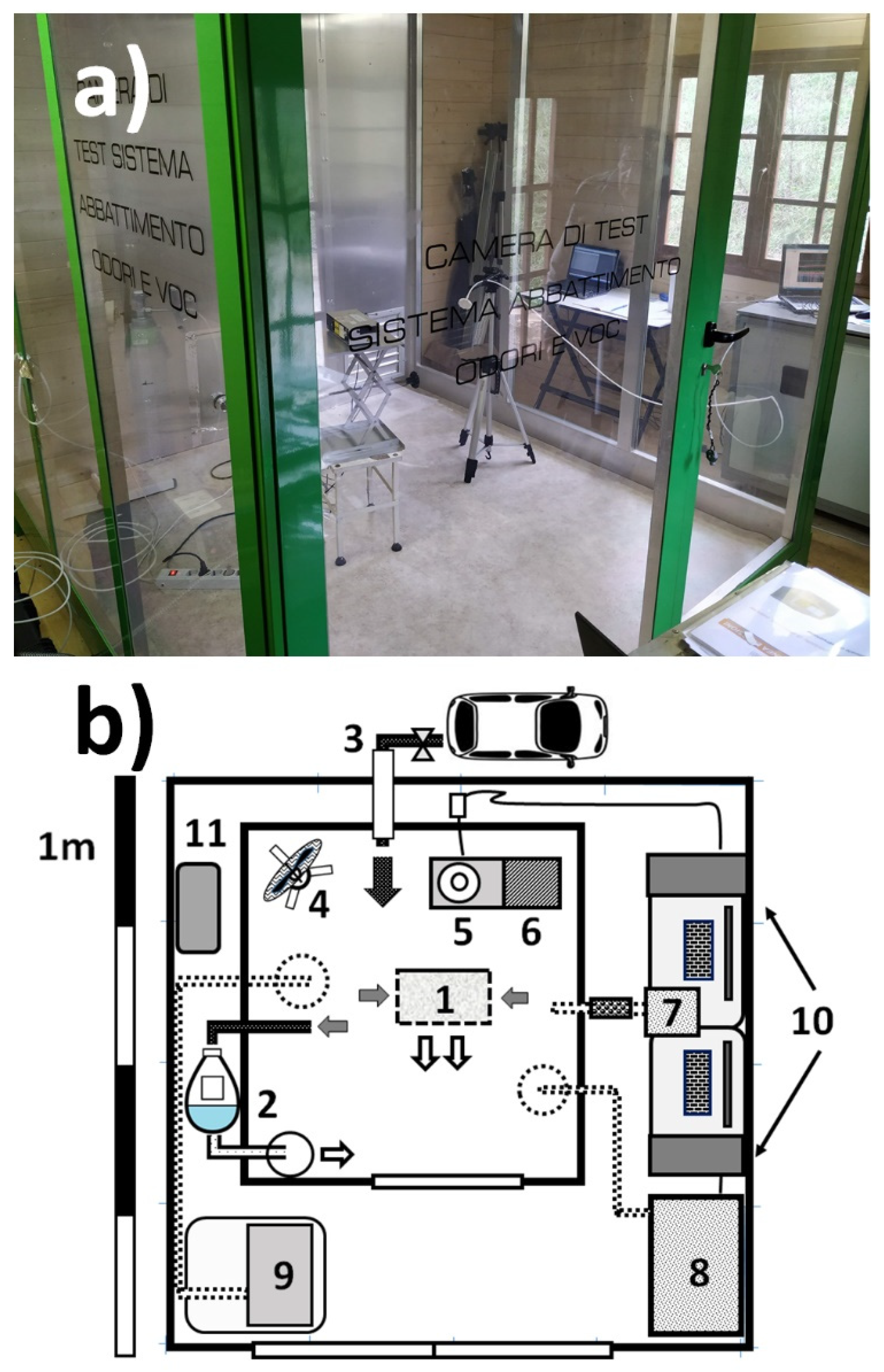
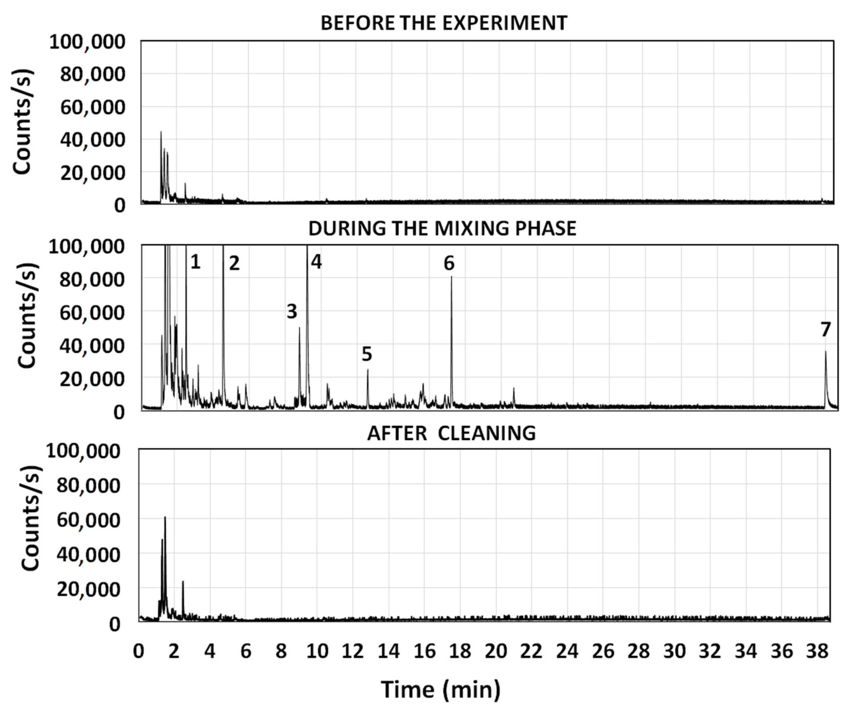
Preliminary experiments were performed to define a testing protocol that could have been extended, with few modifications, to other pollution sources, including cigarette smoke. It was found that enough levels of indoor pollution were generated in the room by delivering the emission from the exhaust pipe of a diesel engine, after having isolated the room from the outdoor environment (phase 2 of Figure 2). This step was performed after the room was cleaned and maintained in communication with ambient air for more than 1 h (phase 1 of Figure 2). This was also the phase when the monitoring of pollutants started. Four minutes of delivering were sufficient to obtain enough indoor pollution to test the performances of a residential air cleaner, by using the exhaust emission of a Euro 3 diesel engine, not equipped with particle filters. Pollutants were generated by keeping the car in the idle mode, and by accelerating the engine from 800 up to 2500 r.p.m. for 4–5 s each minute. This was performed because cold transients produce a much higher emission of pollutants than normal road conditions [32]. As discussed in the following section, indoor pollution at the end of the mixing phase was sufficiently high (PM2.5 from 350–450 μg m−3 and total VOCs from 900–1000 μg m−3) to accurately follow the removal of different pollutants from the room. These levels were 3–5 times higher than those reached at night in the most polluted cities of Europe [7]. Once the desired level of pollution was generated indoors, the line of the exhaust pipe was isolated and the pollutants were allowed to mix inside the room, until a dynamic equilibrium between gases and particles was achieved, producing clear trends in the variation of their indoor levels with the time. The mixing phase might have lasted from 45 min to 4 h, depending on the pollutant. Only in phase 3 of Figure 2, the cleaning device was activated producing a decay of pollutants that was mainly, but not exclusively, produced by the air cleaner and by the working conditions in which it was operated. The removal phase might have lasted from 3–4 h or more, in order to be certain that well-defined decay trends were followed by the various pollutants inside the room. In phase 4 of Figure 2, the cleaning process was stopped, and the persistence of residual pollutants in the room was monitored for 12 h, if needed. In the last phase of the experiment (phase 5 of Figure 2), the room was opened and equilibrated with the outdoor air to observe if the indoor pollution was higher or lower than that existing outdoors. This step allowed us to check that trends of pollutants inside the room were solely determined by indoor equilibria, and no exchanges between the outdoor and indoor air occurred during the entire experiment.
A continuous monitoring was performed to find out how accurately the decay rates of indoor pollutants followed an exponential trend, and their concentrations vs. time were described by the following equation:
C i   i = C O   i   e t   k a i
where k a i is the removal rate constant in h−1 of a pollutant, i, due to a specific removal process, a, in the room; C t i is the concentration of i at a time, t, from the moment when an initial concentration of i   , C O i was present in the room. Plots of l n   C t i vs. time were generated in each experiment because the logarithmic form of Equation (1) can be assimilated to a straight line:
l n   C t i l n C O i = k a i t
where l n   C t i is the intercept, and k a i is the slope. In this way, the decay processes can be quantified, and adequately modeled, by finding the regression lines that fit better with the experimental points.
Since nothing was known about the removal mechanism of the GIOEL system, the first experiments were performed by setting the suction flow rate of air, Φ, at a minimum value of 45 m3 h−1. This allowed us to obtain the highest number of points for the regression analysis. In these conditions, 3.75 air changes per hour (ACPH) occurred in the room, because ACPH = Φ V r , where V r is the volume of the room in m3. To assess the removal rates of particles, a mixing phase lasting 45 min followed by a cleaning phase of 2 h and 45 min was used without replacing the water in the reservoir. At the end of the cleaning phase, particle number concentrations were monitored for more than 12 h before the room was opened.
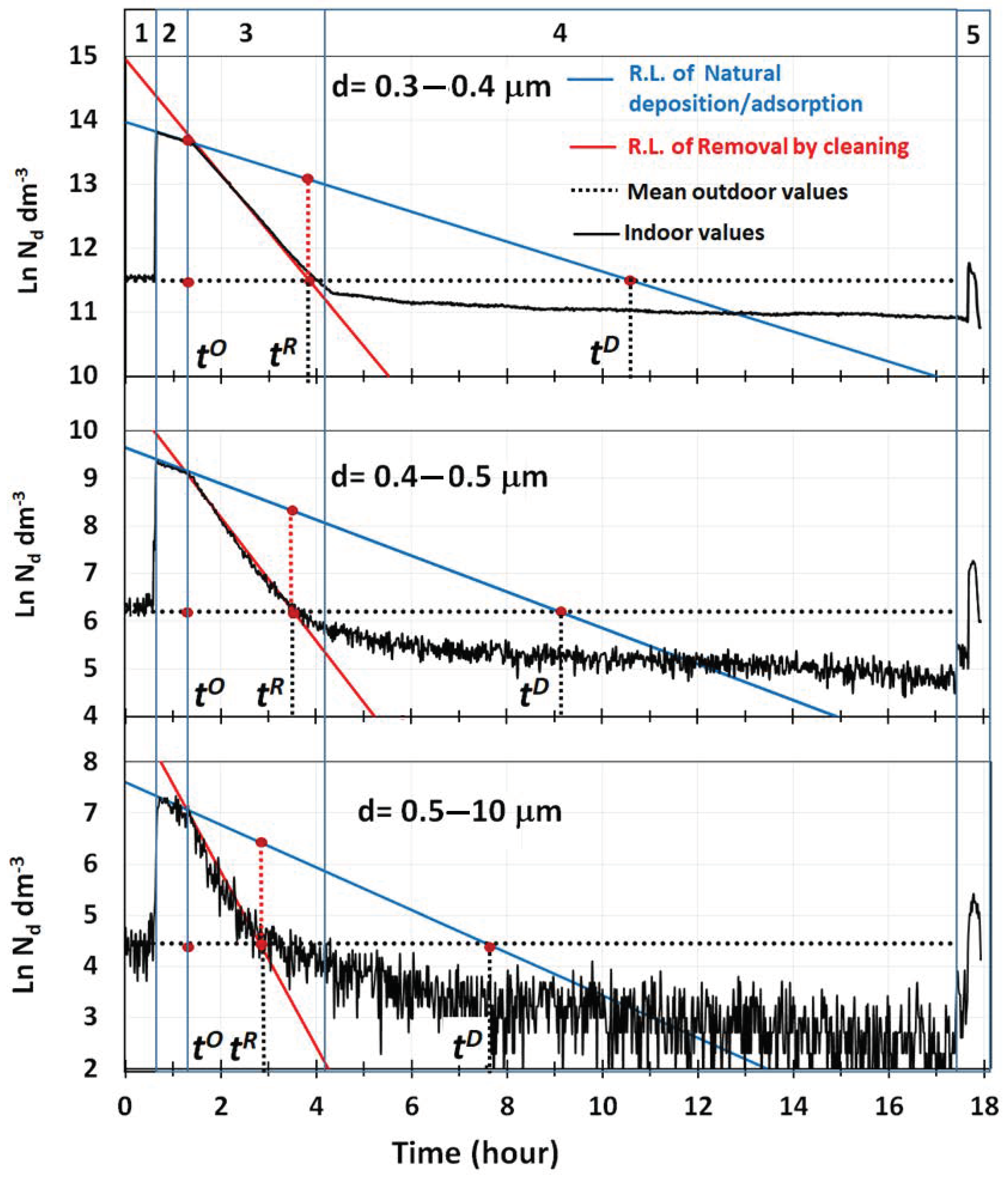
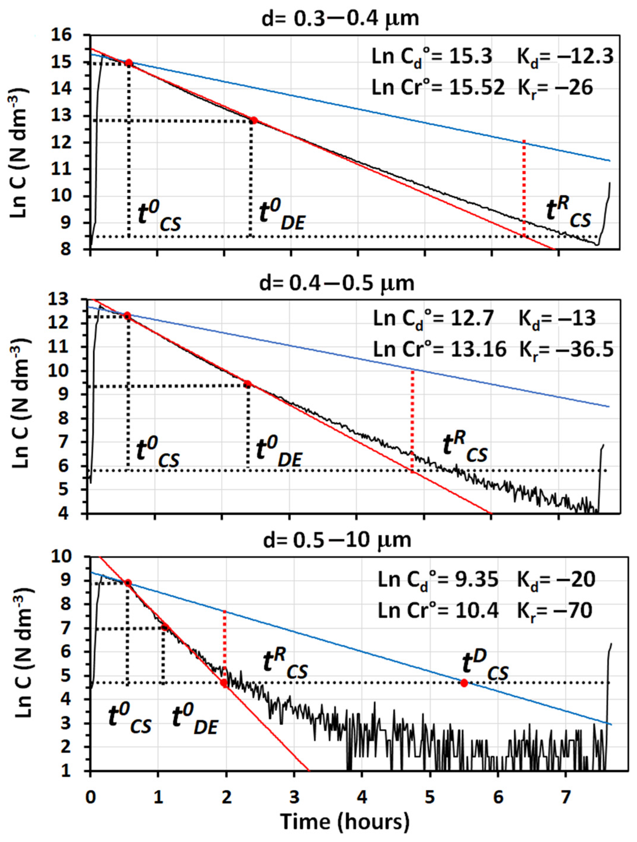
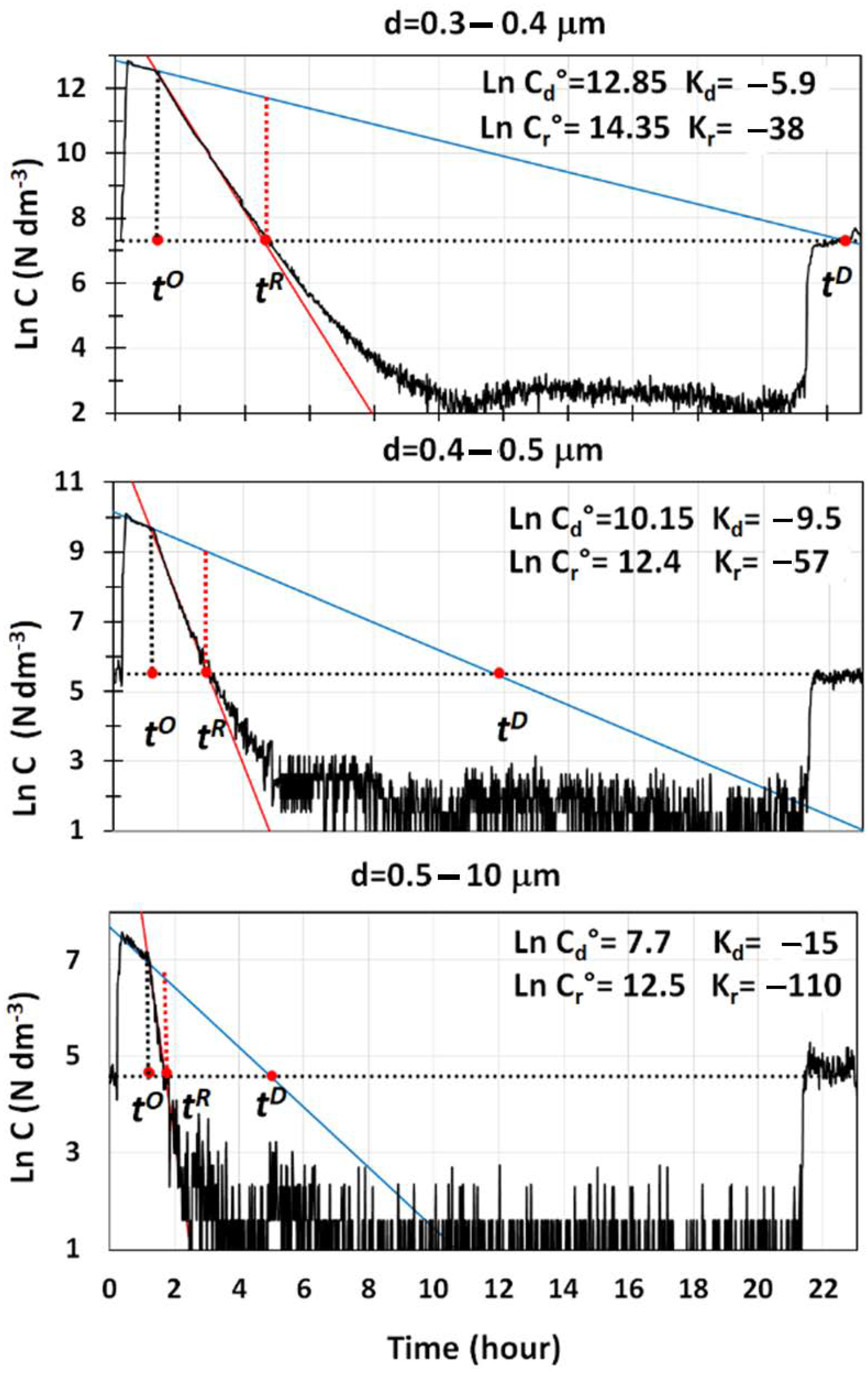
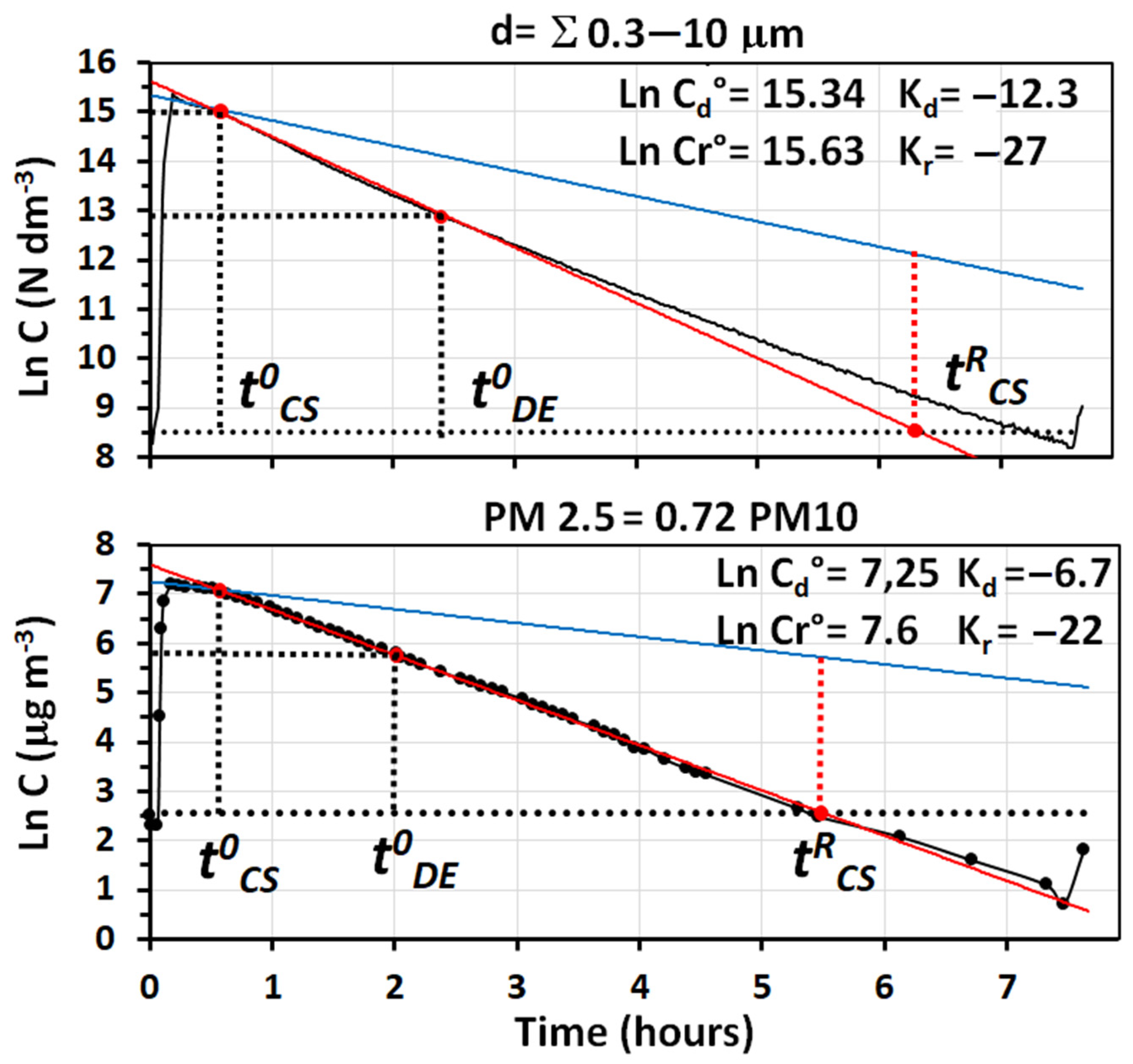
Semi-logarithmic plots of particle number concentrations vs. time for the three main size ranges detected by the OPC are reported in Figure 2, together with the main parameters used to assess the performances of the air cleaner. Two distinct decay trends, closely following Equation (2), were detected, and they were both accurately described by linear regression curves showing a good fit (R2 > 0.998) with the measured values. Regression lines in blue, in Figure 2, describe the removal of particles during the mixing phase, when deposition to the ground and adsorption were the only removal processes active in the room. The values of their intercept and slope are reported in Table 2, in which they are indicated by the subscript d (deposition). In Figure 2 and in Table 2, the intercepts are referred to the starting time of the experiment, t = t I N I T = 0 , which is different from the time, t 0 , used here to indicate the starting time of the removal phase by cleaning. Assessing the removal rates of particles by deposition/adsorption was fundamental, because only by quantifying this contribution was it possible to determine the net removal efficiency of pollutants by the air cleaner.
Data in Figure 2 show that the removal by deposition/adsorption increased with the mean particle size. Since the same density can be assumed for diesel particles, volumes estimated from the mean size diameters are proportional to their mass, indicating that gravitational settling was the process most responsible for the removal of particles inside the room. In spite of the short duration of the mixing phase, the values of the slopes and intercepts of the regression lines obtained in this experiment were the same as those measured when diesel particles were allowed to deposit for more than 16 h in the room.
The removal of particles by water cavitation is described, instead, by the linear regression curves in red in Figure 2, whose intercepts and slopes are reported in Table 2, in which they are indicated by the subscript, r (removal). The black dotted line in Figure 2 indicates, instead, the mean concentrations of particles, ( C A M B ), measured at the beginning and at the end of each experiment, when only atmospheric particles were present in the room at much lower levels than the air quality limits established for the atmosphere. This line, in combination with the pair of regression lines originated at the time, t 0 , allows for the assessment of the net percent removal of a pollutant by the cleaner at any time, t > t 0 .
By inserting into Equation (2) the value of t 0 and those of the slope and intercepts reported Table 2, the initial concentrations of particles at the beginning of the cleaning phase can be obtained, if logarithmic values are converted in their exponential form. At the time, t 0 , C d 1 t 0 = C r 1 t 0 , and this is the value in Figure 2, in which the regression lines by deposition/adsorption across the ones obtained by cleaning are presented.
By accounting for the concentration, C A M B , of atmospheric particles present in the room at the beginning of the experiment ( t = t I N I T = 0 ), the net concentrations of particles to be removed by the cleaner are ( C d 1 t 0 C A M B ) = ( C r 1 t 0 C A M B ) .
If deposition/adsorption is the only removal process active in the room, the net percent removal of particles at any time, t > t 0 , can be calculated as:
[ ( C d 1 t 0 C A M B ) ( C d 1 t C A M B ) ] / ( C d 1 t 0 C A M B ) ] 100
Removal is complete when ( C d 1 t D C A M B ) = 0 , and ( C d 1 t D = C A M B ) , where t D is the time and where the blue lines cross the black dotted line in Figure 2. The time to completely remove particles from the room by deposition/adsorption is thus ( t D t 0 ) .
When removal by cleaning starts in the room, the net percent removal at any given time, t > t 0 , must be calculated with respect to the concentration of particles that survived deposition/adsorption at the time, t . By accounting for them, the net percent removal of particles by the air cleaner is:
[ ( C d 1 t C A M B ) ( C r 1 t C A M B ) ] / ( C d 1 t C A M B ) ] 100
A complete removal occurs when ( C r 1 t R C A M B ) = 0 , and ( C r 1 t R = C A M B ) , where t R is the time in Figure 2, in which the red regression lines across the black dotted ones. The net concentration of particles removed by the cleaner at the time, t R , is indicated in Figure 2 by the dotted vertical segments in red. Based on this, the time required by the cleaner to achieve a complete removal of particles from the room is ( t R t 0 ) < ( t D t 0 ) .
Having clarified the meaning of all curves displayed in Figure 2, and how to use them, we can now discuss the results obtained. They show that diesel particles in the size ranges investigated were all completely removed when the air cleaner was still in operation (phase 3 of Figure 2). The dependence of the decay rates from the mean particle size indicated that, in the experimental conditions used, water cavitation was more efficient in removing particles with a higher mass. The sudden increase in concentrations observed when the room was opened, confirmed that the room was tight enough to maintain sub-ambient levels of particles for quite a long time, and the values of the decay rates reported in Table 2 were not affected by intrusion or ventilation effects. Since no continuous monitoring of PM2.5 and PM10 was performed in this experiment, parallel determinations were carried out indoors and outdoors with the gravimetric method, once the cleaner was switched off. Results obtained by monitoring the particle mass were consistent with those obtained with the particle number, since the indoor value of PM2.5 (5 μg m−3) was 3 times lower than the outdoor one. Using a similar approach, an average concentration of PM2.5 of 402 μg m−3 was found to be present in the room during the mixing phase. By considering that the black carbon particles in diesel emission account for 55 to 70% of the total mass [29], an average concentration of ca. 250 μg m−3 was estimated to be present in the room at the t 0 time, corresponding to a total mass of black carbon particles of ca. 3.23 mg.
Removal rates of VOCs present in the diesel exhaust emission were also determined, but in separate experiments. Since the deposition rates of gases and vapors are usually much lower than those of particles [33], the mixing phase was increased to 4 h and 45 min, and the cleaning phase reduced to 2 h. 
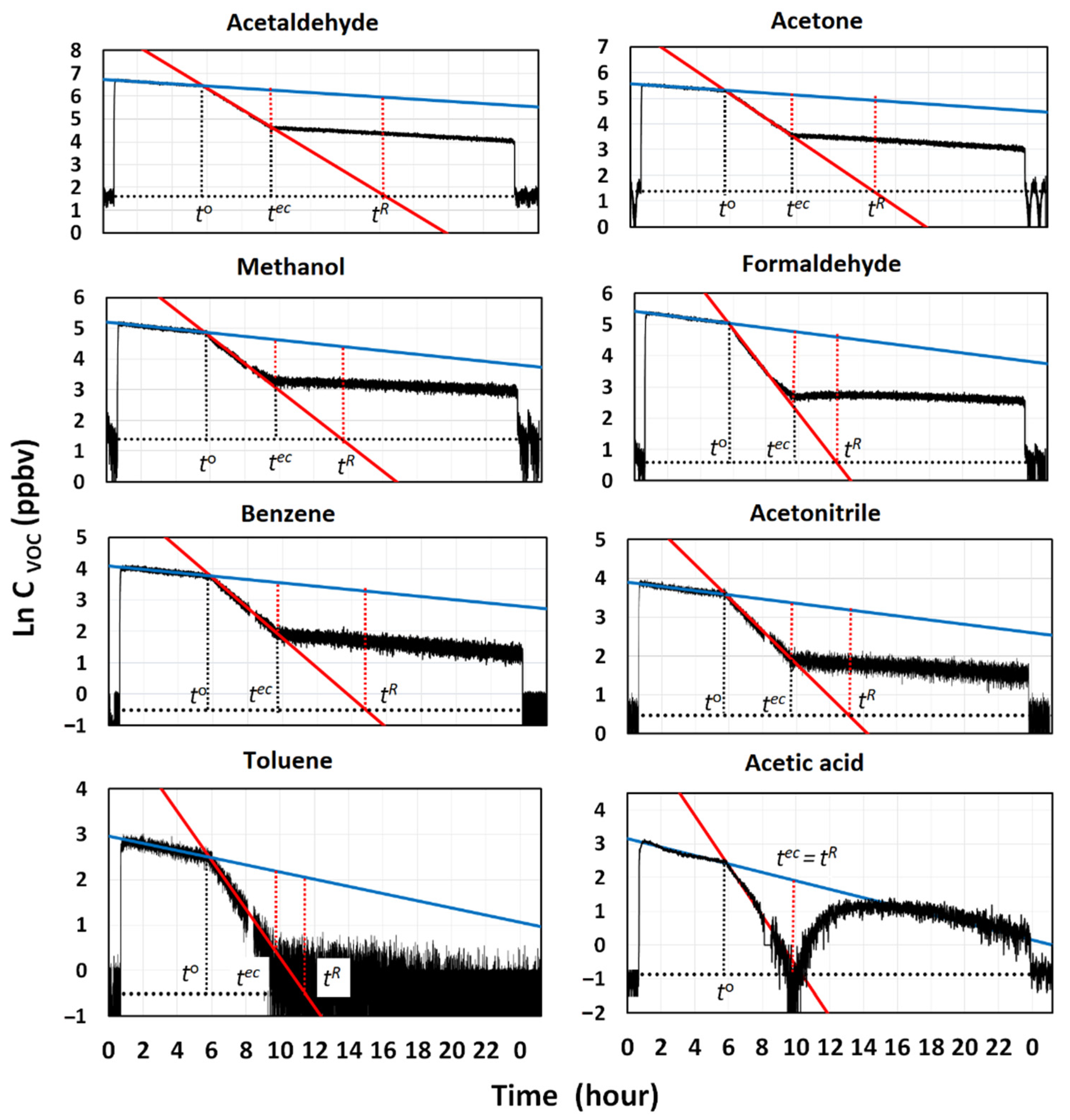
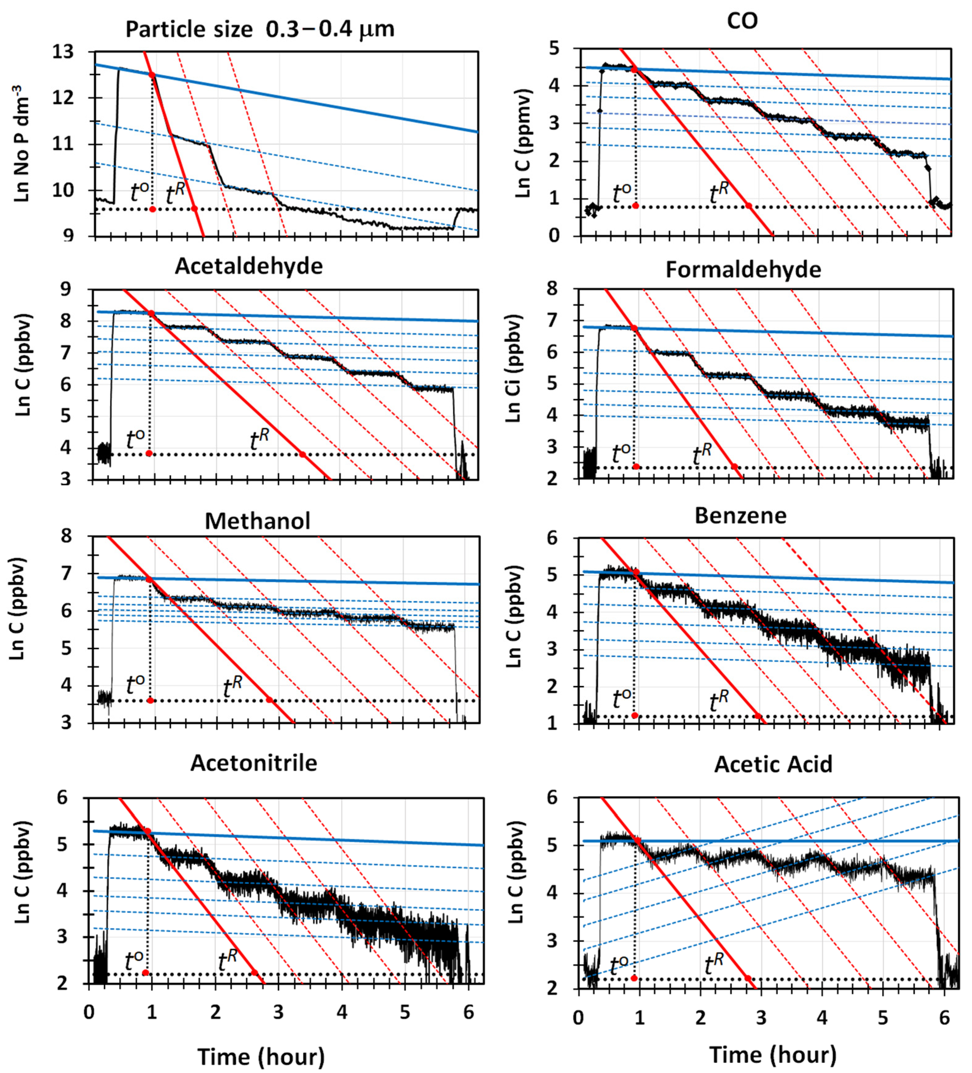
Figure 3 reports the semi-logarithmic plots of the mixing ratios of VOCs vs. time, for the most abundant components sensed by PTR-MS, together with the regression lines generated for the mixing and cleaning phases, and the line indicating the average levels of VOCs measured at the beginning and the end of the experiment. Very accurate regression lines (R2 > 0.998) were obtained for the decay of VOCs in the room. The values of their intercepts and slopes for natural deposition and water cavitation are listed in Table 2. Data consistently show that water cavitation was less efficient in removing VOCs than particles. Except for the acetic acid, not one of the other VOCs was completely removed from the room at the end of the cleaning phase, indicated by the time, t e c , in Figure 3. Thus, the levels higher than those existing outdoors persisted in the room until it was opened, and a sudden drop in the indoor concentrations was observed. The net fractions of VOCs removed by the GIOEL cleaner ranged from 75% to 85%, depending on the VOC type. They can be visually estimated by comparing the lengths of the vertical dotted segments in red, in Figure 3, recorded at the times t R and t e c , respectively. In the experimental conditions used, a time of ( t R t 0 ) 8 h was needed to completely remove all VOCs from the testing room.
The removal rate constants reported in Table 2 showed that the working mechanism of water cavitation was substantially different from a simple dissolution–partition of VOCs in water, because their values were not consistent with the air–water distribution ratio K A W i = C A i C W i , which is a dimensionless form of Henry’s law, in which the concentrations of a species, i , in air, C A i , and in water, C W i , are used. According to this formulation, a compound strongly retained in water by solution–partition is characterized by a very low value of K A W i (typically < 1 × 10⁻⁵), whereas a compound poorly retained in water has values higher than ca. 0.1 [34].
By comparing the values of K A W i , from the literature [34,35], with the removal rate constants reported in Table 2, we can see that a very poorly soluble compound in water, such as benzene (KAW = 0.23), was removed by the GIOEL cleaner at a rate comparable to those of the most highly soluble ones, such as methanol (KAW = 1.82 × 10⁻⁴), acetonitrile (KAW = 8.71 × 10⁻⁴) and acetone (KAW = 1.58 × 10⁻³). This suggests that the removal of VOCs by water cavitation is rather complex, and several phase transitions can take place from the time when bubbles form in the water, until they explode on the surfaces, after having collapsed [25]. It cannot be excluded that the amount and chemical nature of particles can play an important role in the selective removal of VOCs by adsorption and condensation processes.
Data in Figure 3 clearly show that the removal behavior of acetic acid from the room differs from those of the other VOCs. At the end of the experiment, the indoor concentration was higher than the outdoor one, although it was completely removed at the end of the cleaning phase, because of the high solubility in water (KAW = 7.76 × 10⁻⁶) and the capability to stick onto surfaces. The trend followed at the time t > t R , shows that an unexpected increase in concentration occurred. It lasted until the indoor levels matched those of the regression line describing the natural decay of acetic acid by deposition/adsorption. If the removal rate by water cavitation is faster than the kinetics governing the adsorption equilibrium of acetic acid in the room, then a decay in concentration will be observed as long as cleaning is performed. When cleaning ceases, desorption from the room starts to take place, to restore the equilibrium between the gas and the solid surfaces. Adsorption of acetic acid is possible in our case, because it can interact with the [ O C O O R ] n groups of the polycarbonate polymer through hydrogen bonds. If so, adsorption must have occurred at the beginning of the mixing phase (phase 2 in Figure 2), when the highest concentrations of VOCs were reached inside the room.
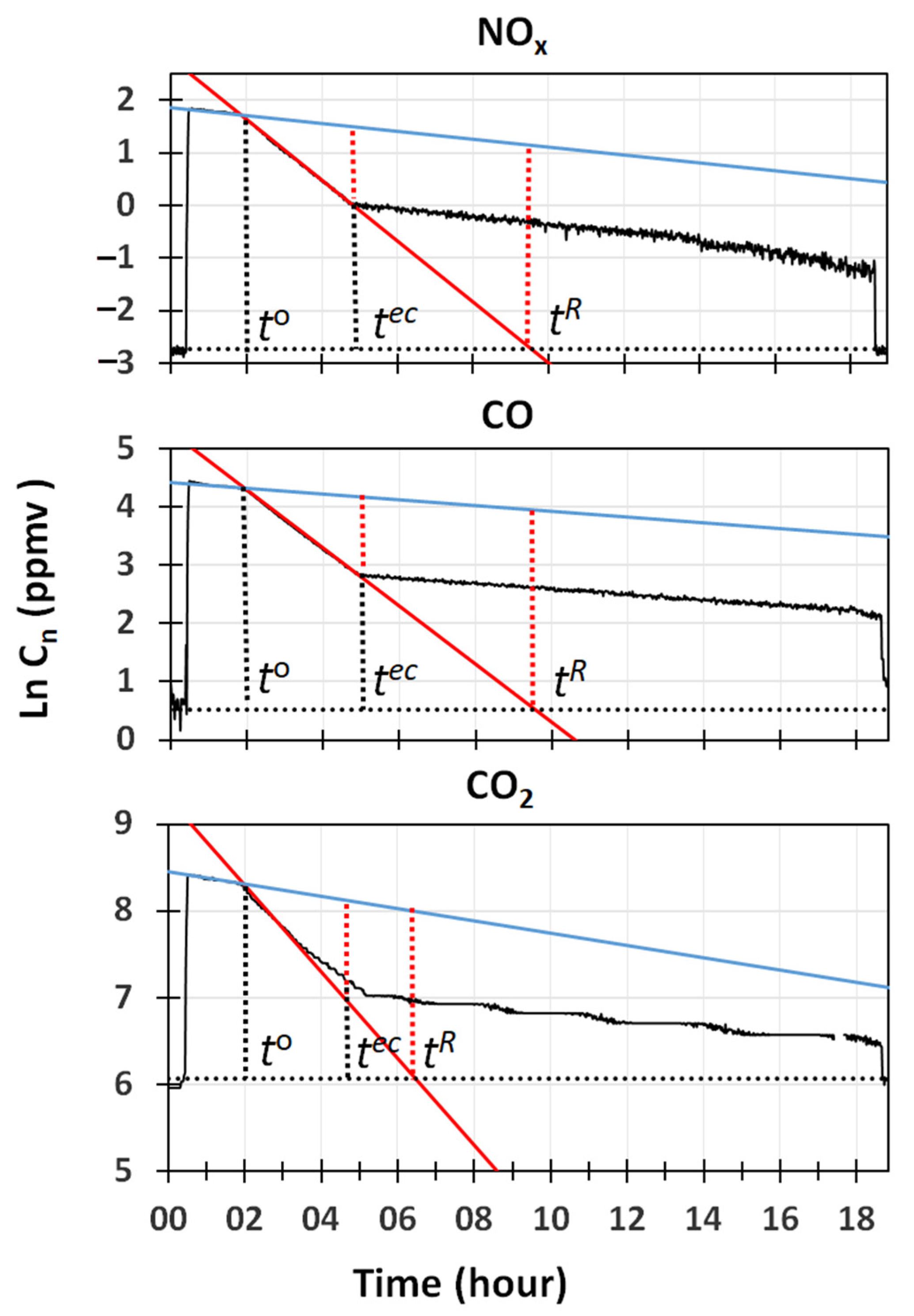
The capability of water cavitation, to remove gases that were nearly insoluble in water, was confirmed by the results displayed in Figure 4. It reports semi-logarithmic plots of l n C t i vs. time for NOx (NO + NO2), CO and CO2, together with the regression lines obtained in the mixing and cleaning phases, and the line indicating the mean concentrations measured at the beginning and the end of the experiment. While an excellent fitting (R2 > 0.998) was obtained for the linear regression curves of CO and NOx, a lower accuracy (R2 = 0.96) was obtained for CO2, due to the stepwise behavior of the sensor used.
Values of the slope and intercepts of the regression lines for the removal by natural deposition/adsorption, and by cleaning obtained for these gases, are also reported in Table 2. Results obtained with CO2 confirmed the unique features of water cavitation. Since CO2 has a much higher solubility in pure water (KAW = 1), than NO (KAW = 20) and CO (KAW = 50), it should have been removed much faster than the other two gases by air–water partition. Removal rates of CO2 can be even higher if a precipitate of calcium carbonate is formed. This was possible in our case, because water with average concentrations of Ca+2 ions between 50 and 99 mg L−1, and a pH between 7.4 and 7.6, was used in all the experiments. Certainly, the removal rates of CO and NOx (that in combustion emission is mainly NO) were quite high, as they were comparable to those of many VOCs that were quite soluble in water. Moreover, in this case, a value of ( t R t 0 )   8 h was required by the GIOEL system to completely remove these gases from the room.
To find out how the suction rate of air affected the removal rates of pollutants by water cavitation, experiments were performed by running the system at the maximum value (180 m3 h−1). In these conditions, the number of ACPH was 4 times higher than in previous experiments. The system was operated in a pulsed mode, by alternating removal phases with mixing phases, for which the system was switched off. This was necessary because, at the highest suction rate, the cleaner cannot run continuously for more than ca. 90 min. The reduction of the water volume in the reservoir is significantly elevated, to strongly limit the water cavitation effect. With the pulsed protocol used, a sufficient number of decay curves for natural deposition/adsorption and water cavitation could have been generated to assess the decay rates of the various pollutants from the room. With this approach, it was also possible to define the most suitable procedure for the collection of water samples for in vitro testing. Since a minimum of 3 water samples needed to be collected for each experiment, and ca. 10 min was necessarily required to obtain the sample, clean the water reservoir and to refill it with fresh water, the pulsed experiment also allowed us to check how regular and predictable the decay trends of pollutants in the room were, when no flow of air was passing through it.
Figure 5 reports the semi-logarithmic plots of ln C t i vs. time, for the most significant pollutants recorded in the room when 5 removal steps of 20 min were alternated with mixing phases of 35 min. As shown in Figure 5, a stepwise trend in concentration was followed by all pollutants. The decay was so clear, that it was possible to clearly distinguish when removal by cleaning and by mixing occurred. The trends of the pollutants were so well described in Equation (2), that it was possible to generate regression lines for the removal by deposition/adsorption and by cleaning for any time, t n 0 , when cleaning started. The fitting of the regression lines with the experimental points was good enough (0.998 < R2 < 0.988), that reliable values of the slopes and intercepts were obtained for each one of the cleaning and mixing steps performed in the pulsed experiment. To make it easier to read the curves in Figure 5, it is important to remember that only one regression line for the removal by natural deposition/adsorption and one for the removal by cleaning are generated at each time, t n 0 . In a regular pulsed mode, each pair of regression lines is also related to those generated at the time, t 0 , because t n 0 = t 0 + n t N , where n is the number of removal steps assuming the first equals to 0, and t N the time interval between each removal step (35 min in our case).
From the observation of the regression lines generated in the various removal steps, indicated by the red lines in Figure 5, we can see that their parallelism is so close that, by setting t N = 0, they all combine into the curve generated at t 0 . Under these conditions, the regression line generated at t 0 is formally equivalent to the one generated when the air cleaner is run in a continuous mode. The values of the slopes and intercepts of the t 0 regression lines for the removal by cleaning obtained for the various pollutants investigated are reported in Table 3, in which they are indicated by the subscript, r. By comparing them with the values reported in Table 2, it can be observed that a 4 time increase in the ACPH produced a significantly variable increase in the removal rate constants of the various pollutants, with values ranging from 1.4 to 4.6. The fact that a 3.8 increment was observed for some particles and many VOCs, suggests that the Φ V r ratio strongly affects the value of k a i . This effect can be better expressed by observing that k a i   ( Φ V r ) α i , where αi is an adimensional term, ranging from 0.3 to 1, measuring the impact of water cavitation on the species, i . Values of t R   identified by these regression lines, provide an estimate of the time ( t R t 0 ) necessary to completely remove a pollutant from the room, if the cleaner was run on a continuous mode. From the data displayed in Figure 5, a time of ca. 2 h was needed to remove all the pollutants from the room, with respect to the 8 h necessary when the cleaner was continuously run at the minimum airflow rate.
These conclusions hold, if the regression lines by deposition/adsorption, indicated in blue in Figure 5, also combine into the one obtained at the time, t 0 . This occurs if all regression lines generated at any time, t n 0 , show a decrease in the initial concentrations that match the amount removed by the cleaner in the previous removal step, and such a difference is maintained during all the mixing steps. In geometrical terms, all regression lines generated at any time, t n 0 , must be parallel to that generated at the time, t 0 , and properly downscaled in their initial concentrations by the amount removed in each cleaning step.
Data in Figure 5 show that these conditions were met by all compounds, except the acetic acid. The values of the slopes and intercepts of the regression lines obtained at t 0 , for deposition/adsorption, are reported in Table 3, in which they are indicated by the subscript, d. Decay rates by natural deposition/adsorption measured in the pulsed mode were generally lower than those reported in Table 2; however, with the only exception being represented by the acetic acid, the differences were sufficiently small to not substantially affect the value of the net percent removal of various pollutants by the air cleaner.
Results obtained in the pulsed experiment confirmed that the desorption of acidic acid from the room occurred, and it was not negligible. As shown in Figure 5, the regression line generated at the time, t 0 , was characterized by the same small negative slope than the other VOCs, whereas those generated in the following mixing steps all showed a positive slope with a constant value of 9 h−1, correlating well with the experimental points (R2 > 0.98). These results confirmed that the emission of acetic acid was slower than the removal by water cavitation, for which a value of −38 h−1 was measured. As shown in Figure 5, the duration of the mixing step was significantly long, that the amount of acetic acid released at any step, t n   0 > t 0 , almost matched that removed by the air cleaner. The net effect was that the amount of acetic acid removed from the room at the end of the experiment, was not so much lower than that removed by natural deposition/adsorption.
Based on the ( t R t 0 ) value for acetic acid, shown in Figure 5, the desorption effects could have been eliminated by running the air cleaner in a continuous mode for more than 2 h. Since this was not possible, a pulsed protocol was designed to limit the desorption effects as much as possible. It consisted of 3 removal steps of 40 min, alternated with 3 mixing steps of 10 min. This protocol allowed for the collection of 3 water samples in the time interval, between t R and t 0 , in addition to the one collected when the room was opened to the outdoor air for 1 h. Decay curves recorded in this pulsed experiment were fully consistent with those displayed in Figure 5, with the only difference that 2 removal steps were combined into 1, and mixing reduced by 1/3. The release of acetic acid was still visible, but it was sufficiently low, so that the regression lines by cleaning did not differ too much from the t 0 regression line in red, in Figure 5. The complete removal of VOCs from the room, at the end of the experiment, was confirmed by a parallel sampling performed indoors and outdoors on traps, later analyzed by GC-MS. Results obtained confirmed that the indoor levels of VOCs were lower than those measured outdoors. The parallel sampling of PM2.5 and PM10 also confirmed that the indoor levels of particles were smaller than those existing outdoors, and they were consistent with the data provided by the OPC.
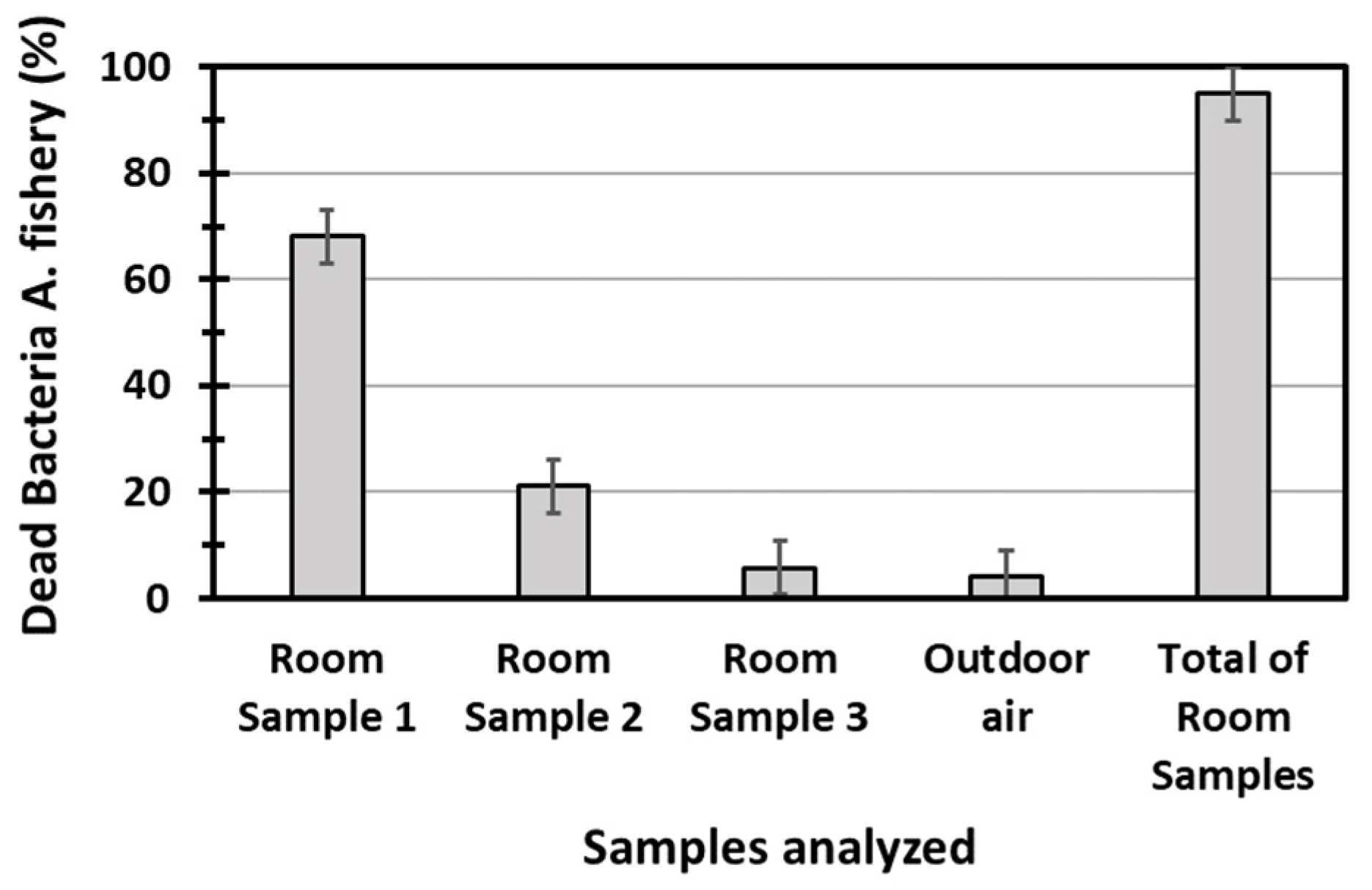
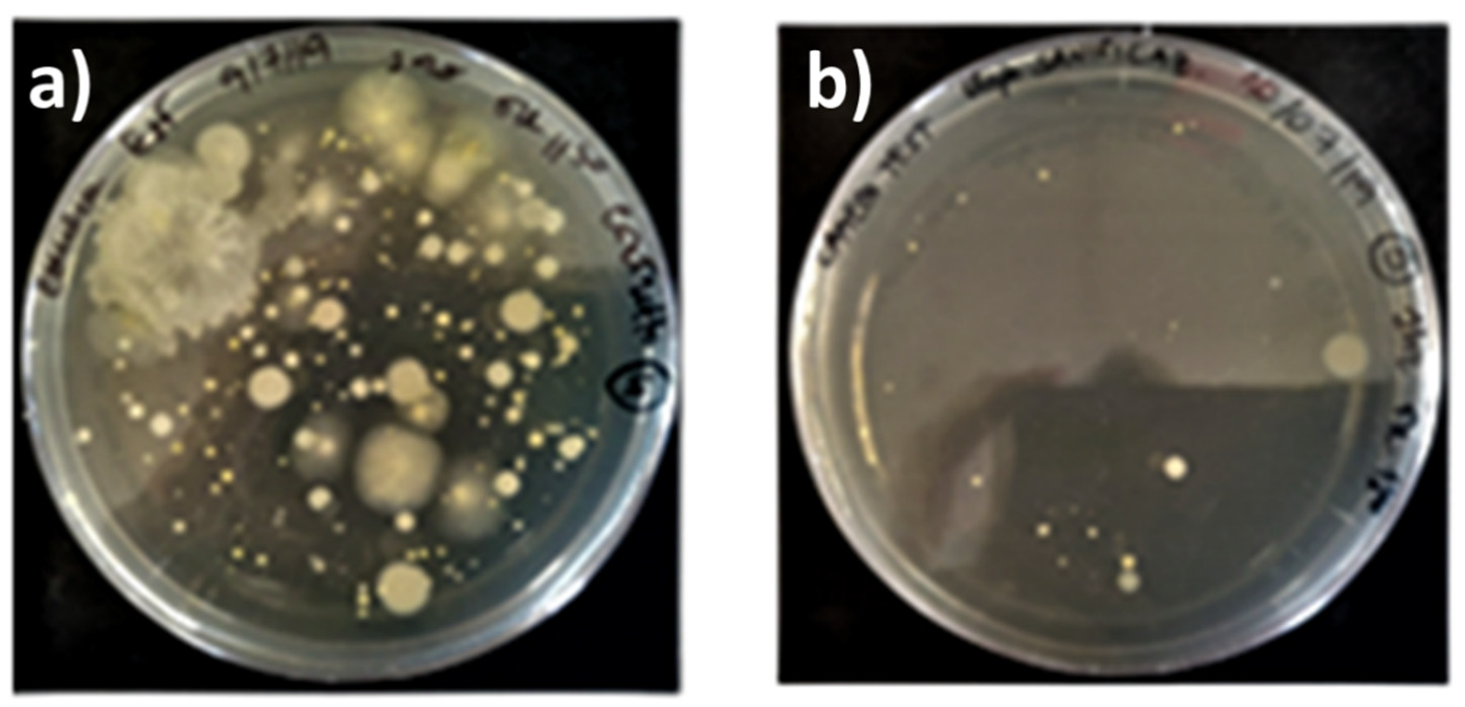
Figure 6 reports the dead fractions of the bioluminescent bacteria of Allivibrio fischeri, measured by submitting the water samples collected in the pulsed experiment to the Microtox® test. The value of the total toxicity, obtained by mixing equal aliquots of the first three samples collected in the room, is also reported in Figure 6.
Results reported in Figure 6 show that that the total toxicity of diesel exhaust emission was significantly elevated, that 95% of the bacteria were killed by the toxic substances contained in the emissions collected in a single experiment, estimated to be in the range of 5.2–5.5 mg. As indicated by the bar graphs in Figure 6, 70% of the toxicity was concentrated in the first 40 min sample, whose collection started at t 0 . In this sample, more than 80% of the particles were concentrated, based on the black deposit, 2 cm wide, that was accumulated in the areas of the reservoir in which the bubbles exploded. The volume of black particles appeared to be consistent with the amount of ca. 3.3 mg, estimated in the previous experiment. SEM analysis showed that the deposit was mostly made by large aggregates of fine black carbon particles, where sparse atmospheric particles of pollen were present, together with well-developed crystals of calcite, probably formed by calcium carbonate precipitation in water. The second 40 min sample showed a limited toxicity, mostly determined by VOCs and inorganic gases, as the deposition of black particles in the reservoir was just visible. The last 40 min sample showed a toxicity that, within the experimental errors, was the same as that of outdoor air. The decay trend of toxicity vs. time, followed an exponential decay, with a slope of −1.85 h−1 when plotted in a semi-logarithmic scale. This represents quite a noticeable decay, if we consider the limited sensitivity scale of the Microtox® test. The results suggest that the GIOEL system could have been used as a sampler to assess the capability of any other cleaning system, providing that the diesel exhaust emission is used as a pollution source.

3.1.2. Checking the Performances of Prototypes for Possible Improvements

The study performed on the SANINDOOR prototype, provides an example of how the room was used to check if a cleaning system meets the requirements defined in the technical project, or if improvements are needed before the system is put into production.
In contrast with the GIOEL system, the SANINDOOR prototype was designed to run continuously until the indoor levels in a room reached the air quality standards defined for the atmospheric air. The air cleaner was also designed to remove those organic and inorganic compounds, such as methyl mercaptan and H2S, producing annoyance because of their intense, malodorous smell. With this cleaner the removal of pollutants is obtained by combining the effects of different filtering agents exploiting adsorption, with a stage in which VOCs are oxidized to CO2 by gaseous oxidants generated in two sequential steps, in which the final one is a photochemical flow reactor. Using the US-EPA classification [15], the air cleaner can be classified as a combination of systems using adsorption on fiber filters, plasma and photolysis. The company did not provide information about the way that these modules work, as they can be modified before the final system is produced. The only information available was that it presently operates at a flow rate of 380 m3 h−1 (19–33 ACPH in our room). In addition to the removal of particles and VOCs, the system must have been tested for the removal of NO2 and the ozone (O3) production. When the system was in operation, the indoor levels of O3 must have been comparable to those present in the outdoors (35–40 ppbv). To maintain these levels, the system was programmed to automatically reduce the O3 production by 50%, if indoor levels in the room exceeded 35 ppbv. Since no specific modules for the removal of CO2 were present in the cleaner, no removal of this gas from the room was expected to occur during the cleaning phase. Thus, the decay of CO2 was assumed to be the same as that described by the regression line for the deposition/adsorption reported in Figure 4. This was reasonable because the levels of CO2 generated by diesel exhaust emission at the time, t 0 , were so high (3 × 10³ and 4 × 10³ ppmv), that any possible removal or production by the cleaner (estimated in the order of ±10 ppmv) could have never detectably changed the behavior of this gas in the room.
Given the complex oxidation system used, a high number of VOCs was monitored. The reliability of solid-state sensors for total VOCs and PM2.5 and PM10 was also tested. Since many companies use these types of sensors to control their air cleaners, it was important to know how their signals fitted with those provided by other methods. This was particularly true for sensors measuring the total VOC content, whose real meaning is not yet clear. Since formaldehyde is, by definition, a VOC, (it is indeed an organic compound with a vapor pressure at ambient conditions higher than 0.13 kPa [36]), the use of a specific sensor for this compound conflicts with term used to identify any total VOC type of sensors. Furthermore, it cannot be excluded that such sensors poorly detect other very volatile compounds.
The protocol followed with the SANINDOOR prototype was the same as that used with the GIOEL system, with the only difference being that the air cleaner was run continuously for 16 h, after the mixing phase. Figure 7 reports the semi-logarithmic plots of particle number concentrations vs. time recorded in the room, during an experiment performed with diesel exhaust emissions. The size ranges reported are the same as in Figure 2. Together with the regression lines determined in the mixing and removal phases of the experiment, the values of their intercepts and slopes are also reported in Figure 7. By neglecting the data of natural deposition, that were essentially the same as those reported in Table 1 and Table 2, the decay rates by cleaning obtained with the SANINDOOR prototype were sufficient to remove all particles recorded by the OPC in about 3 h; although, only the particles in the greatest size range were removed at the same rate as water cavitation working at the maximum speed.
Furthermore, in this case, the removal efficiency increased with the particle size. This was consistent with the fact that larger particles are better retained on fiber filters by impaction.
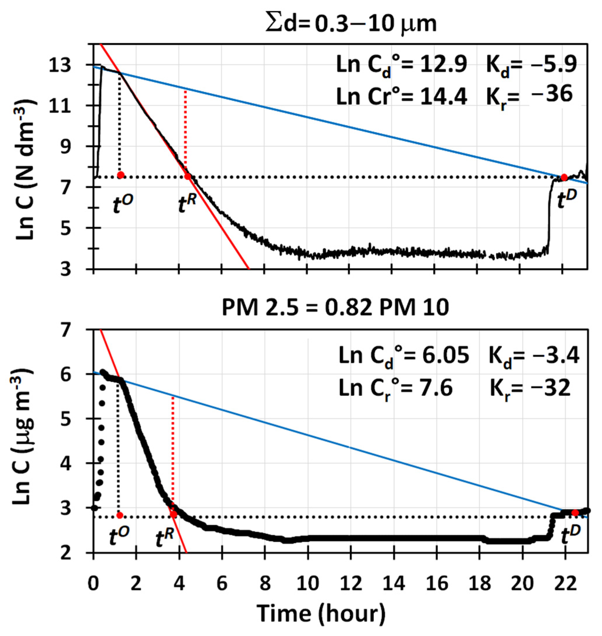
The removal efficiency of the system can be fully evaluated, by looking at the data reported in Figure 8, in which the semi-logarithmic plot vs. time of total particle number concentration sensed by the OPC is compared to that obtained by monitoring the total particle mass. In this experiment, the values of PM2.5 and PM10 were determined with two different solid state-sensors, one from PCE and the other from Tea Group, whose responses were previously calibrated with the gravimetric method.
Data in Figure 8 show that the air cleaner can reduce the initial concentrations of PM2.5 in the room, from 388 μg m−3 to ambient levels (ca. 16.5 μg m−3) in ca. 3 h, and levels as low as 5–6 μg m−3 are maintained until the room is opened. It is worth noting that the curves obtained by the two solid state sensors, measuring PM2.5 and PM10, agreed so well that only one is reported in Figure 8. By considering that the indices measured by the two types of monitors are different and that the instruments used are also different, a satisfactory agreement was found between the decay curves obtained using particle number and particle mass concentrations.
As far as VOCs are concerned, attention was concentrated on 14 chemical species that, although present at levels ranging from more than 100 ppbv to 0.01 ppbv, were all considered as crucial to test the working mechanism of the air cleaner. This was justified by the fact that some VOCs, such as methyl butadiene, are quickly oxidized by common atmospheric oxidants (such as ozone and OH radicals) to form methacrolein (MAC), methyl vinyl ketone (MVK) and formaldehyde [9], whereas others, such as benzene, methanol, acetonitrile and acetone, are only slowly and partly oxidized by them [9]. 
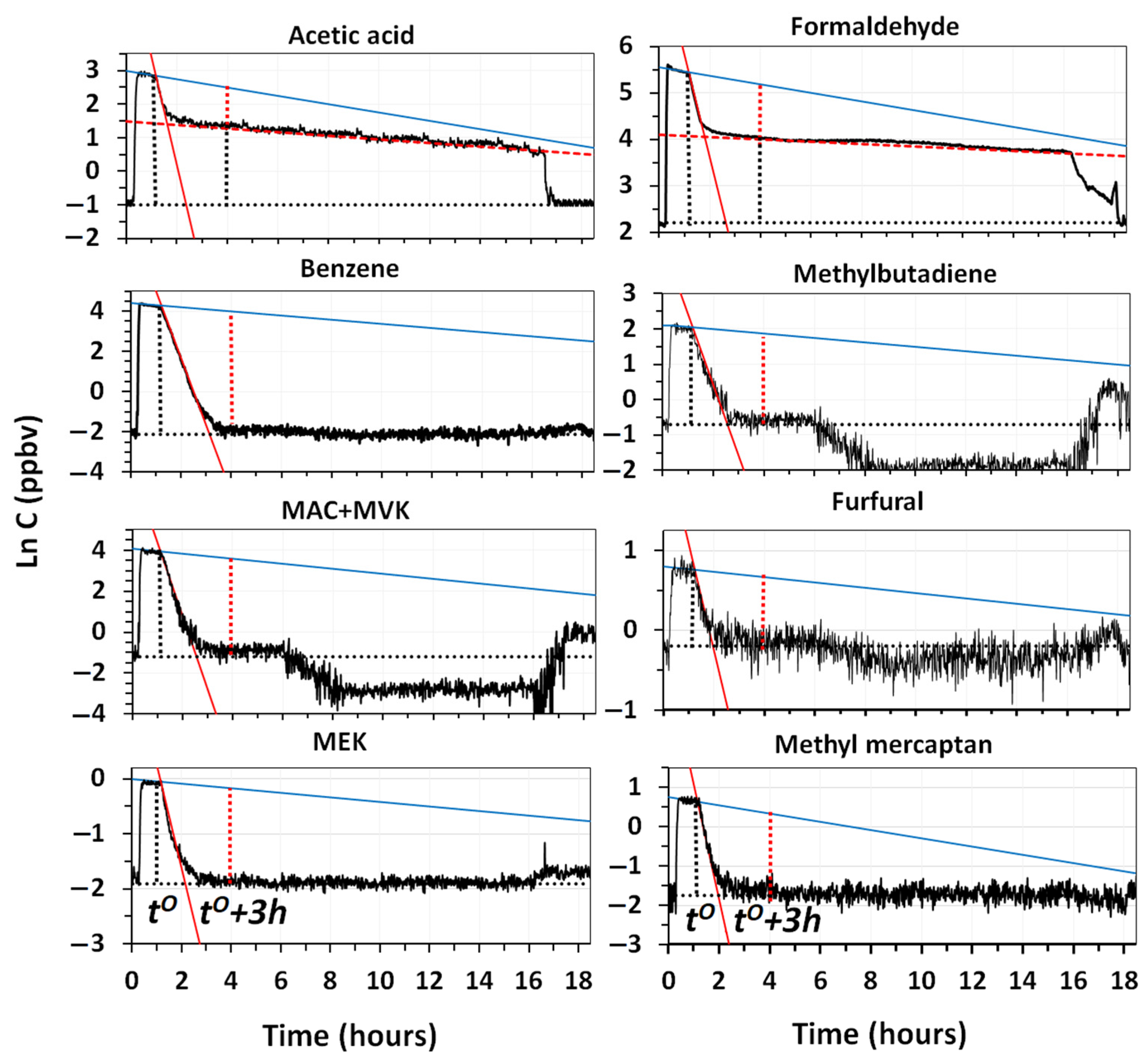
Figure 9 reports the decay trends of selected VOCs measured in the room, in a diesel experiment lasting 16 h.
As shown in Figure 9, some compounds were only partly removed by the system after 3 h of cleaning, whereas others were already totally removed within this time interval. During the experiment, some of them reached values much lower than the outdoor ones, confirming that ventilation or penetration effects did not affect the equilibrium inside the room. Information provided by curves in Figure 9, are complemented with those reported in Table 4, in which the values of the intercepts and slopes of the regression lines are obtained for natural deposition/adsorption, and for the removal by cleaning are listed. Table 4 also reports the values of the regression lines obtained using the solid-state sensor of total VOCs, together with the net fraction of each VOC removed by the system, after 3 h of cleaning.
The results show that the lowest removal efficiency was reached by methanol and acetaldehyde, whereas values higher than 60% were obtained for the other most volatile VOCs (acetone, acetonitrile, acetic acid and formaldehyde). The result for methanol was somehow expected, since it is very hard to remove by adsorption on the fiber filters, even if coated with carbon, and, similar to acetonitrile and acetone, it is poorly oxidized by ozone and OH radicals [9]. Instead, all compounds with a molecular weight higher than methacrolein (70 g mol−1) were completely removed from the room in less than 3 h, although some of them, such as MAC and MVK, were certainly produced by the oxidation of methyl butadiene and other reactive olefins. The higher percent removal of formaldehyde, in respect to acetaldehyde and methanol, indicated that the specific module to convert formaldehyde into CO and CO2 worked, to some extent, especially if we consider that the high levels of this pollutant present in diesel emissions are further increased by the oxidation of methyl butadiene and of many other olefins, such as ethylene and 2–3 butadiene [9]. The removal of benzene, toluene and xylenes + ethylbenzenes, indicated that the filtration module of the system performed quite well. The use of the same filter, for more than one year, did not show any release of these toxic compounds from it.
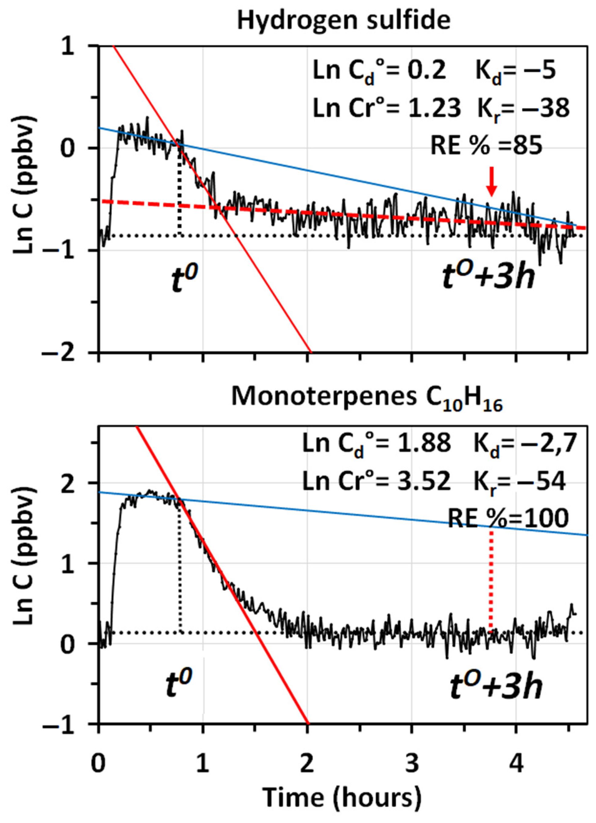
The complete removal of the most odorous compounds (furfural and methyl mercaptan) released by diesel emissions was particularly important. The high sensitivity afforded by PTR-MS, allowed us to accurately observe the removal of methyl mercaptan from the room, in spite of the very low concentrations (2.2 ppbv) present at the time, t 0 . High sensitivity was fundamental in this case, since the odor threshold of methyl mercaptan is only 0.07 ppbv [37]. Although a signal of H2S was detected, it was too small to assess the net percent amount removed by the cleaner. This compound is important because its odor threshold is also rather low (0.41 ppbv) [37].
Data in Table 4, show that total VOC content determined with solid-state sensors was somehow consistent with that obtained by PTR-MS, and this index, together with that of PM10 and/or PM2.5, would have allowed us to compare the performances of the prototype system with those of the air cleaners in the market that are equipped with the same type of sensors. To obtain a more comprehensive view of the removal of VOCs, the suite of solid-state sensors should definitely include that for the monitoring of formaldehyde, as it provided results not too different to those obtained with PTR-MS, and with the electrochemical sensor we used.
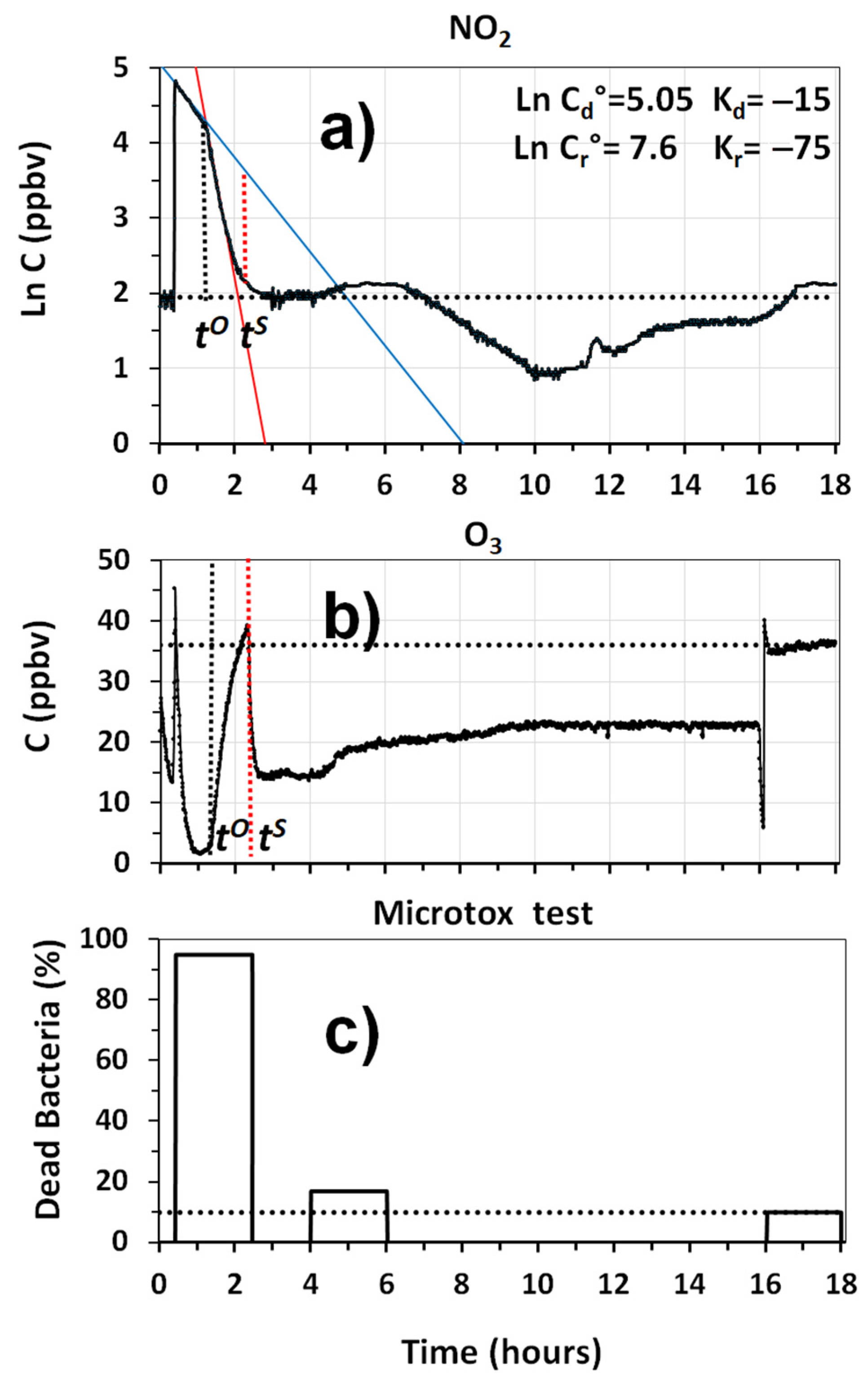
Data on the removal of NO2 and the production of O3 were also obtained in a separate experiment. Results reported in Figure 10a, show that the system was able to rapidly remove NO2 from the room, although a continuous production of this pollutant must have occurred by the reaction of NO with the O3 produced by the plasma. This effect is clearly visible from the strong decay of O3, when NOx was introduced into the chamber, as shown in Figure 10b. Once the titration of O3 by NO decreased, the O3 levels in the room started to increase until a value of 35 ppbv was exceeded. At this point, indicated as t s in Figure 10b, the internal regulation of the O3 production was automatically activated, cutting the amount of O3 produced by the system by 50%. This avoided the exceedance of 40 ppbv of O3 in the room, and allowed us to keep the indoor levels in the range of 20 ppbv for the rest of the experiment.
Figure 10c provides information on the capability of the prototype to remove toxic substances from the room. It reports the results of the Microtox® tests performed on water samples collected with the GIOEL system, during different phases of the experiment. Data show that the toxicity of the sample, collected after 3.5 h from the beginning of the experiment, was much smaller than that measured during the mixing phase, because the fraction of dead bacteria was in the range of 17%, which is a value that is only 7% higher than that present in the outdoor air. This means that the cleaning system was able to remove 78 to 80% at least, of toxic substances, sensitive to this microbial test, that were present in diesel exhaust emissions. Although satisfactory, these results can be improved in what concerns the removal of some VOCs, especially formaldehyde. Further work should be conducted, to implement the performances of two of the modules present in the air cleaner.

3.2. Cigarette Smoke and Other Emission Sources

Although diesel exhaust emission was an excellent source to test the removal of toxic pollutants with different air cleaners, it has some practical limitations. If too much emission is delivered into the chamber, ultrafine particles tend to rapidly grow by nucleation and aggregation, preventing an accurate determination of their removal rates by deposition/adsorption and by cleaning. As shown in Figure 5 and Figure 7, the maximum value of the initial concentration at the time, t 0 , ranged between 370 and 420 μg m−3 of PM2.5. This, combined with the fact that the emission of some VOCs was also limited, suggested that cigarette smoke must have also been tested. In addition to being highly toxic, cigarette smoke has a size distribution of particles centered at ca. 0.3 μm [38], fitting better with the minimum size range observed by our OPCs. The protocol was the same as that used with diesel exhaust emissions, the only difference being that the mixing phase started when the operator went outside the room, when a sufficient amount of pollution was generated inside the room. For the sake of comparison, experiments were performed with the same SANINDOOR prototype used in the experiments of Figure 7 and Figure 8, but limited the cleaning time to less than 8 h.
Figure 11 reports the semi-logarithmic plots of particle number concentrations vs. time measured in the room, when cigarette smoke was used as a pollution source. In the same figure, the values of the intercepts and slopes of the regression lines for the removal by deposition/adsorption and by cleaning are reported, together with the line indicating the mean outdoor values measured at the beginning and the end of the experiment. The size ranges investigated were the same as those shown in Figure 7. Data in Figure 11, show that cigarette smoke allowed us to follow the decay rates of particles in a much wider concentration range than diesel exhaust emissions, and, in particular, of the fraction higher than 0.5 μm. Differences between the two emission sources can be estimated by observing the initial concentrations measured at t C S 0 and t D E 0 , where the subscripts CS and DE refer to cigarette smoke and diesel exhaust particles, respectively. The results show that both removal rates by deposition/adsorption, and by cleaning, increased with the size range of the particles. This was consistent with the fact that large particles are deposited faster by gravitational settling, and better removed by impaction on the filter. However, the removal rates of particles by deposition/adsorption were higher than those measured with the diesel particles, whereas the removal rates by cleaning were lower. This indicated that cigarette smoke particles were more difficult to remove by the air cleaner than diesel particles. The linear regression lines obtained in the removal phase of cigarette smoke particles did not show the same accuracy as those obtained with diesel particles, making the value of the time ( t C S R t C S 0 ) needed to completely remove particles from the room less precise. The differences between the estimated and measured values of t C S R were more visible in the smaller size range investigated.
In Figure 12, the semi-logarithmic plots vs. time of the total particle number concentrations are compared with those obtained by monitoring the particle mass concentration in the PM2.5 range. Plots are analogous to those reported in Figure 8, for diesel particles. Data show that the concentration reached by cigarette smoke particles in the room at the time t C S 0 (1330 μg m−3), was about 4 times higher than that reached by diesel particles (380–400 μg m−3) in previous experiments, whose values correspond to the time indicated as t D E 0 in Figure 12. Concentrations reached by cigarette smoke particles were so high, that the abatement devices developed to remove particles from industrial sources could have also been tested in our room.
Furthermore, Figure 12 shows that the regression line describing the removal of PM2.5 by cleaning, better fitted with the measured values, than those obtained with particle number concentrations. This suggests that, for the aerosol type of particles emitted from cigarette smoke, PM2.5 is a more reliable index to predict the time, t R , when a complete removal of particles is obtained. By comparing the data reported in Figure 7 with those shown in Figure 12, we can observe that the time ( t R t 0 ) necessary to completely remove the same initial amount of PM2.5 particles from the room was 20–25% shorter than when diesel particles were used as a pollution source, confirming the lower efficiency of the air cleaner to remove the aerosol type of particles.
Since the initial VOC concentrations generated in the room by cigarette smoke did not substantially differ from those generated by diesel exhaust emissions, the data reported in Table 4 can be used for them. The only additional information obtained by using cigarette smoke emissions, was that it was possible to assess the removal rate of monoterpenes and H2S from the room. Data in Figure 13, show the semi-logarithmic plots of the concentration of total monoterpenes and H2S vs. time, which were measured when the room was polluted with cigarette smoke emissions. Together with the initial outdoor concentrations and regression lines for the removal by deposition/adsorption and by cleaning, Figure 13 also reports the values of the intercepts and slopes of the regression lines, and the net percent removal measured after 3 h of cleaning. The results show that the air cleaner was able to remove H2S to quite a large extent, and completely removed monoterpenes from the room within 3 h. A complete removal of monoterpenes was important because they can produce O3 and secondary organic particles (SOA) by indoor oxidation [10,11].
To verify if other VOCs not observed by PTR-MS were also completely removed by the cleaning system, cartridges were collected in the room at the times t I N , t 0 and ( t 0 + 3 h )   , which were later analyzed by GC-MS. Figure 14 shows the GC-MS profiles of VOCs obtained in this experiment. The results show that the sample collected after 3 h of cleaning, was quite deprived of semi-volatile compounds with a molecular weight higher than monoterpenes, with the only exception being represented by a compound identified as 3,5-dimethyl cyclohexanol. The lack of nicotine and nicotyrine, detected in the smoke sampled after the cigarette filter, suggested that, in the temperature conditions of the room (25 °C ± 3 °C), these VOCs were mostly in the aerosol phase, and they were completely removed by the cleaning system.
GC-MS determinations also confirmed that only the most volatile VOCs detected by PTR-MS were the ones partly removed by the air cleaner.
The aerosol nature of the emission did not allow the assessment of the toxicity removed by the system using the Microtox® bioassay. The net removal of the VOCs, particles and inorganic gases by the GIOEL cleaner, were much lower (20–30%) than those obtained with diesel exhaust emissions. This confirmed the crucial role played by the soot in the removal of pollutants by water cavitation. It is possible that aerosols were vaporized during the bubble production, and, at the highest sucking rate used, they were unable to condense on the wall reservoir, after having collapsed. This aspect certainly needs further investigations.
Resuspended particles from agricultural soils were also used as a pollution source in the room, following the same basic protocol adopted with the diesel emissions. This natural source contained sufficient amounts of bacteria and molds that were detected with both passive and active sampling on Petri dishes filled with a growing medium. Figure 15 shows the colonies of bacteria and mycelia detected during the mixing phase, and after the removal of particles from the room. Tests were performed with the SANINDOOR prototype as an air cleaner, because the GIOEL system was already certified for the removal of these air contaminants.
Through counting, it was found that the air cleaner removed 85 ± 5% of bacteria and 75% ± 4% of mycelia from the room. No presence of pathogenic bacteria, such as Pseudomonas aeruginosa, Escherichia coli or Enterococcus faecalis, was detected, so bacteria were mostly non-pathogenic. The mycelia belonged to the Cladosporium, Alternaria and Aspergillus genera. The fact that they are very common in indoor environments, indicates that resuspended agricultural soil was a good source to assess their removal by cleaning.
Sampling of resuspended soil particles performed with the GIOEL system, allowed us to control how many bacteria were still alive after the treatment made with SANINDOOR prototype. Results showed that only 20% of them survived the cleaning. This suggested that, in spite of the limited O3 production, the content of oxidants produced by the air cleaner was still able to largely inertize the bacteria. The oxidative properties of the SANINDOOR prototype were confirmed by the fact that it was also able to inhibit the growth of Escherichia coli by 70%. Since the bacterium was spiked on the growing medium of a Petri dish, these experiments were performed when the particles were completely removed from the room.

4. Conclusions

The results obtained show that the testing room developed in this study is a quite versatile tool to investigate different aspects of the removal processes of indoor pollutants by residential air cleaners. Diesel exhaust emission, cigarette smoke and other emission sources were successfully used for testing. The use of diesel exhaust emission allows the quantification of the fraction of the toxic substances responding to the Microtox® test that are removed by any cleaner. This result has been achieved because water samples were collected at various stages of the removal process, using an air cleaner exploiting the water cavitation effect as a sampler. The almost real-time detection achieved by PTR-MS, allows us to determine, with a high accuracy, the removal rates of different VOCs from the room by natural deposition/adsorption and by cleaning, and to predict when and to what extent the air cleaner removes them. The room allows the assessment of the levels of VOCs, O3 and NO2 produced and/or removed by cleaning systems using cold plasma and photochemical flow reactors to remove indoor pollutants. Although the results obtained in the room might not always truly reflect what happens in a real indoor environment, they provide the fundamental scientific basis necessary for their further testing.
Recently, the room has been successfully used to assess the emission rates of particles, aldehydes and VOCs from the sawing of wood in indoor environments, by implementing the instrumental panoply available to the chamber.

Author Contributions

Conceptualization: P.C. (Piero Ciccioli), P.C. (Paolo Ciccioli), C.R. and P.S.; methodology: P.C. (Paolo Ciccioli), P.C. (Piero Ciccioli), E.P., E.G., M.A.I., E.D. and C.R.; Software: E.P., E.G., L.L., P.C. (Piero Ciccioli) and P.C. (Paolo Ciccioli); validation: P.C. (Paolo Ciccioli), P.C. (Piero Ciccioli) and R.M.; investigation, P.C. (Paolo Ciccioli), P.C. (Piero Ciccioli), E.P., E.G., M.A.I., E.D. and C.R.; resources, C.R., P.S. and P.C. (Paolo Ciccioli); data curation, P.C. (Paolo Ciccioli), P.C. (Piero Ciccioli) and R.M.; writing—original draft preparation: P.C. (Paolo Ciccioli), P.C. (Piero Ciccioli) and R.M.; writing—review and editing, R.M.; supervision, P.C. (Paolo Ciccioli); project administration, C.R. and P.C. (Paolo Ciccioli); funding acquisition, C.R., P.C. (Paolo Ciccioli) and P.S. All authors have read and agreed to the published version of the manuscript.

Funding

This research was partly funded by LazioInnova, which is the research funding Agency of the Latium Region, Rome, Italy, through the SANINDOR Project, Grant no A0112-2016-13301, CUP F17H18000080007, within the frame of the competitive call LIFE 2020 POR FESR launched by the Lazio region for the years 2014–2020.

Institutional Review Board Statement

Not Applicable as it does not involve humans or animals.

Informed Consent Statement

Not Applicable as it does not involve humans or animals.

Acknowledgments

The authors wish to thank Paola Grenni of the Istituto di Ricerca sulle Acque del CNR (IRSA-CNR) for the determination of live and dead bacteria in water samples, and Loredana Caccavale of IRET-CNR for the sampling and GC.MS analyses of VOC samples.

Conflicts of Interest

All the CNR authors and co-authors of this paper declare that no additional funding other than that provided to CNR by LazioInnova, the funding Agency of the Latium Region, has been provided to anyone of them by the GIOEL S.p.A. and RI.EL.CO Ambiente S.r.l., in any possible form that can represent potential conflicts of interest between the authors.

References

  1. Gonzalez-Martín, J.; Lebrero, R.; Kraakman, N.J.R.; Perez, C.; Munoz, R.A. state-of-the-art review on indoor air pollution and strategies for indoor air pollution control. Chemosphere 2021, 262, 128216–128276. [Google Scholar] [CrossRef]
  2. Guyot, G.; Sherman, M.H.; Walker, I.S. Smart ventilation energy and indoor air quality performance in residential buildings: A review. Energy Build. 2018, 165, 416–430. [Google Scholar] [CrossRef] [Green Version]
  3. Carazo Fernandez, L.; Fernandez Alvarez, R.; Gonzalez-Barcala, F.J.; Rodríguez Portal, J.A. Indoor air contaminants and their impact on respiratory pathologies. Arch. Bronconeumol. 2013, 49, 22–27. [Google Scholar] [CrossRef] [PubMed]
  4. Leung, D.Y.C. Outdoor-indoor air pollution in urban environment: Challenges and opportunity. Front. Environ. Sci. 2015, 2, 69. [Google Scholar] [CrossRef]
  5. Chan, A.T. Indoor-outdoor relationships of particulate matter and nitrogen oxides under different outdoor meteorological conditions. Atmos. Environ. 2002, 36, 1543–1551. [Google Scholar] [CrossRef]
  6. Stull, R.B. An Introduction to Boundary Layer Meteorology; Springer: Dordrecht, The Netherlands, 1998. [Google Scholar] [CrossRef]
  7. Ciccioli, P.; Cecinato, A.; Brancaleoni, E.; Frattoni, M.; Zacchei, P.; Miguel, A.H.; De Castro Vasconcellos, P. Formation and transport of 2-nitrofluoranthene and 2-nitropyrene of photochemical origin in the troposphere. J. Geophys. Res. Atmos. 1996, 101, 19567–19581. [Google Scholar] [CrossRef]
  8. Finlayson-Pitts, B.J.; Pitts, J.N., Jr. Tropospheric air pollution: Ozone, airborne toxics, polycyclic aromatic hydrocarbons, and particles. Science 1997, 276, 1045–1052. [Google Scholar] [CrossRef] [Green Version]
  9. Finlayson-Pitts, B.J.; Pitts, J.N., Jr. Chemistry of Upper and Lower Atmosphere; Academic Press: San Diego, CA, USA, 2000. [Google Scholar] [CrossRef]
  10. Nørgaard, A.W.; Kudal, J.D.; Kofoed-Sørensen, V.; Koponen, I.K.; Wolkoff, P. Ozone-initiated VOC and particle emissions from a cleaning agent and an air freshener: Risk assessment of acute airway effects. Environ. Int. 2014, 68, 209–218. [Google Scholar] [CrossRef] [Green Version]
  11. Nørgaard, A.W.; Kofoed-Sørensen, V.; Mandin, C.; Ventura, G.; Mabilia, R.; Perreca, E.; Cattaneo, A.; Spinazzè, A.; Mihucz, V.G.; Szigeti, T.; et al. Ozone-initiated terpene reaction products in five European offices: Replacement of a floor cleaning agent. Environ. Sci. Technol. 2014, 18, 13331–13339. [Google Scholar] [CrossRef]
  12. Campagnolo, D.; Saraga, D.E.; Cattaneo, A.; Spinazzé, A.; Mandin, C.; Mabilia, R.; Perreca, E.; Sakellaris, I.; Canha, N.; Mihucz, V.G.; et al. VOCs and aldehydes source identification in European office buildings—The OFFICAIR study. Build. Environ. 2017, 115, 18–24. [Google Scholar] [CrossRef]
  13. Samson, R.A. Occurrence of molds in modern living and working environments. Eur. J. Epidemiol. 1985, 1, 54–61. [Google Scholar] [CrossRef]
  14. Andualem, Z.; Gizaw, Z.; Bogale, L.; Dagne, H. Indoor bacterial load and its correlation to physical indoor air quality parameters in public primary schools. Multidiscip. Respir. Med. 2019, 14, 2–7. [Google Scholar] [CrossRef] [Green Version]
  15. Guide to Air Cleaners at Home. Portable Air Cleaners, Furnace and HVAC, 2nd ed.; EPA-402-F-08-004; EPA Indoor Environment Division: Washington, DC, USA, 2008. Available online: https://19january2017snapshot.epa.gov/indoor-air-quality-iaq/residential-air-cleaners-second-edition-summary-available-information_.html#summary (accessed on 20 February 2021).
  16. Residential Air Cleaners. A Technical Summary. Portable Air Cleaners, Furnace and HVAC, 3rd ed.; EPA-402-F-09-002; EPA Indoor Environment Division: Washington, DC, USA, 2018. Available online: http://www.epa.gov/iaq (accessed on 20 February 2021).
  17. Method for Measuring Performance of Portable Household Electric Room Air Cleaners—ANSI/AHAM AC-1-2020; Association of Home Appliance Manufacturers (AHAM): Washington, DC, USA, 2020.
  18. Independent Air Purification Devices for Tertiary Sector and Residential Applications—Test Methods—Intrinsic Performances, 2016; AFNOR-NF B44-200; Association Française de Normalisation (ANFOR): Saint-Denis, France, 2016; Available online: https://www.afnor.org/en (accessed on 18 June 2021).
  19. Japan Electrical Manufacturer Association (JEMA). Residential Air Cleaners, JEM 1467; Japan Electrical Manufacturer Association (JEMA): Tokyo, Japan, 1995. [Google Scholar]
  20. Ciccioli, P.; Cecinato, A.; Brancaleoni, E.; Draisci, R.; Liberti, A. Evaluation of Nitrated Polycydic Aromatic Hydrocarbons in Anthropogenic Emission and Air Samples: A Possible Means of Detecting Reactions of Carbonaceous Particles in the Atmosphere. Aerosol Sci. Technol. 1989, 10, 296–310. [Google Scholar] [CrossRef]
  21. Szulczyński, B.; Gębicki, J. Currently Commercially Available Chemical Sensors Employed for Detection of Volatile Organic Compounds in Outdoor and Indoor Air. Environments 2017, 4, 21. [Google Scholar] [CrossRef] [Green Version]
  22. Lusini, I.; Pallozzi, E.; Corona, P.; Ciccioli, P.; Calfapietra, P. Novel application of a combustion chamber for experimental assessment of biomass burning emission. Atmos. Environ. 2014, 94, 117–125. [Google Scholar] [CrossRef] [Green Version]
  23. Ciccioli, P.; Brancaleoni, E.; Frattoni, M. Sampling of atmospheric volatile organic compounds (VOCs) with sorbent tubes and their analysis by GC-MS. In Environmental Monitoring Handbook; Burden, F.R., Kelvie, I.M., Guenther, U.F.A., Eds.; Mc Graw-Hill: New York, NY, USA, 2002; Volume 21, pp. 1–85. Available online: https://www.accessengineeringlibrary.com/content/book/9780071351768 (accessed on 18 June 2021).
  24. Johnson, B.T. Microtox® Acute Toxicity Test. In Small-scale Freshwater Toxicity Investigations; Blaise, C., Férard, J.F., Eds.; Springer: Dordrecht, The Netherlands, 2005; pp. 69–105. [Google Scholar] [CrossRef]
  25. Brennen, C. Cavitation and Bubble Dynamics; Cambridge University Press: Cambridge, UK, 2013. [Google Scholar] [CrossRef] [Green Version]
  26. Pitts, J.N., Jr.; Grosjean, D.; Mischke, T.M.; Simmon, V.F.; Poole, D. Mutagenic activity of airborne particulate organic pollutants. In Biological Effects of Environmental Pollutants; Lee, S.D., Mudd, J.B., Eds.; Ann Arbor Science Publishers: Ann Arbor, MI, USA, 1997; pp. 219–235. [Google Scholar]
  27. Hiroyuki, Y.; Misawa, K.; Suzuki, D.; Tanaka, K.; Matsumoto, J.; Fujii, M.; Tanaka, K. Detailed analysis of diesel vehicle exhaust emissions: Nitrogen oxides, hydrocarbons and particulate size distributions. Proc. Combust. Inst. 2011, 33, 2895–2902. [Google Scholar] [CrossRef]
  28. Andreae, M.O.; Merlet, P. Emission of trace gases and aerosols from biomass burning. Global Biogeochem. Cycles 2001, 15, 955–966. [Google Scholar] [CrossRef] [Green Version]
  29. Burtscher, H. Physical characterization of particulate emissions from diesel engines: A review. J. Aerosol Sci. 2005, 36, 896–932. [Google Scholar] [CrossRef]
  30. Guerin, M.R.; Higgins, C.E.; Jenkins, R.A. Measuring environmental emissions from tobacco combustion: Side-stream cigarette smoke literature review. Atmos. Environ. 1987, 21, 291–297. [Google Scholar] [CrossRef]
  31. Gariazzo, C.; Carlino, C.; Silibello, C.; Renzi, M.; Finardi, S.; Pepe, N.; Radice, P.; Forastiere, F.; Michelozzi, P.; Viegi, G.; et al. BEEP Collaborative Group1. A multi-city air pollution population exposure study: Combined use of chemical-transport and random-Forest models with dynamic population data. Sci. Total Environ. 2002, 724, 138102. [Google Scholar] [CrossRef]
  32. Di Lorenzo, A.; Polletta, A.; Ciccioli, P.; Brancaleoni, E.; Cecinato, A. Emission of PAH from a light-duty diesel car as a function of the operating conditions: A possible approach for investigating the parameters affecting the formation of toxic components in soot. In Polynuclear Aromatic Hydrocarbons. Measurements, Means and Metabolism; Cooke, M., Loening, K., Merritt, J., Eds.; Battelle Press: Columbus, OH, USA, 1991; pp. 239–258. [Google Scholar]
  33. Pacyna, J.M. Atmospheric deposition. In Encyclopedia of Ecology; Academic Press: San Diego, CA, USA, 2008; pp. 275–285. [Google Scholar] [CrossRef]
  34. Hilal, S.H.; Ayyampalayam, S.N.; Carreira, L.A. Air-liquid partition coefficient for a diverse set of organic compounds: Henry’s Law Constant in water and hexadecane. Environ. Sci. Technol. 2008, 42, 9231–9236. [Google Scholar] [CrossRef] [PubMed]
  35. Sander, R. Compilation of Henry’s law constants (version 4.0) for water as solvent. Atmos. Chem. Phys. 2015, 15, 4399–4981. [Google Scholar] [CrossRef] [Green Version]
  36. Bloemen, H.J.T. Editor Introduction to: Chemistry and Analysis of Volatile Organic Compounds in the Environment; Bloemen, H.J.T., Burn, J., Eds.; Blackie Academic & Professional: Glasgow, UK, 1993; pp. 1–2. [Google Scholar] [CrossRef]
  37. Nagata, Y. Measurement of odor threshold by triangle odor bag method. Odor Meas. Rev. 2003, 118, 118–127. [Google Scholar]
  38. Sahu, S.; Tiwari, M.; Bhangare, R.; Pandit, G. Particle Size Distribution of Mainstream and Exhaled Cigarette Smoke and Predictive Deposition in Human Respiratory Tract. Aerosol Air Qual. Res. 2012, 13, 324–332. [Google Scholar] [CrossRef] [Green Version]
Figure 1. (a) Picture of the testing room. (b) Map showing the position of the instruments, air cleaners and emission sources: (1) air cleaner operating indoors; (2) air cleaner operated from outdoors; (3) line to introduce car exhaust emissions and resuspended soil particles; (4) fan; (5) optical particle counters; (6) monitors for PM2.5, PM10, total VOCs, formaldehyde and NO2; (7) samplers to collect VOCs on sorbent tubes; (8) PTR-MS; (9) monitor of O3, NOx, CO and CO2; (10) data acquisition systems; and (11) air conditioning system. Dotted lines = sampling lines. Dotted lines with circles = sampling lines passing from the top of the ceiling.
Environments 09 00003 g001
Figure 2. Semi-logarithmic plots of the particle number concentrations vs. time recorded in the testing room for three of the size ranges investigated. Data refer to the experiments performed with diesel exhaust emission using the GIOEL air cleaner run at the minimum speed. Numbers at the top of the graphs refer to the various phases of the experiment: (1) room under ambient atmospheric conditions; (2) introduction and mixing of pollutants into the room (mixing phase); (3) activation of the cleaning device (removal phase); (4) end of the removal phase; and (5) room opening and end of the experiment. Blue solid line = regression line for natural deposition/adsorption, red solid line = regression line for the removal by cleaning, and horizontal black dotted line = mean outdoor concentration. RL = regression line; t 0 = starting time of cleaning; t D = time when 100% particles are removed by deposition/adsorption; and t R = time when 100% of particles are removed by air cleaning.
Environments 09 00003 g002
Figure 3. Semi-logarithmic plots of the mixing ratios of selected VOCs vs. time recorded in the testing room in the experiments performed with diesel exhaust emission, using the GIOEL air cleaner run at the minimum speed. The meaning of the lines and of the symbols are the same as in Figure 2. Vertical dotted segment in black = net amount of VOC to remove, and vertical dotted segment in red = net amount removed by the cleaner. The time ted = ending time of cleaning.
Environments 09 00003 g003
Figure 4. Semi-logarithmic plots of the of the mixing ratios of NOx, CO and CO2 vs. time recorded in the testing room during the experiments performed with diesel exhaust emission, using the GIOEL air cleaner run at the minimum suction rate of air. The meaning of the lines and symbols is the same as in Figure 3.
Environments 09 00003 g004
Figure 5. Semi-logarithmic plots of selected pollutants vs. time recorded in testing room during the pulsed experiment performed with diesel exhaust emission using the GIOEL air cleaner at the maximum flow rate. The meaning of the lines and symbols are the same as in the previous figures. The various curves identify the pair of regression lines that were generated at each cleaning step according to a pulsed sequence t n 0 = t 0 + n t N , where n = number of steps, t N the time between the steps and t 0 the initial steps indicated in the thick solid line in red, in the figure.
Environments 09 00003 g005
Figure 6. Toxicity levels measured with the Microtox® test, performed on the water samples collected in the testing room during a pulsed experiment performed with diesel exhaust emission. Sampling was performed by passing the air through the GIOEL cleaner operated at the maximum suction rate for 40 min. Room samples, numbered from 1 to 3, were collected at a 10 min interval one from the other. The outdoor sample was collected after the room was maintained for more than 1 h, in communication with the outdoor atmosphere.
Environments 09 00003 g006
Figure 7. Semi-logarithmic plots of particle number concentration vs. time recorded, in the experiment performed with diesel exhaust emission using the SANINDOR prototype as air cleaner. The meaning of the lines and symbols are the same as in Figure 2, Figure 3 and Figure 4. Values of the slopes and intercepts of the regression lines for natural deposition/adsorption (d) and by removal by cleaning (r), are reported in the figure. They are calculated with the value of t = 0, indicated in the text as t I N .
Environments 09 00003 g007
Figure 8. Semi-logarithmic plots of total particle number concentration and PM2.5 vs. time recorded in the testing room during the experiment performed with diesel emission, using the SANINDOR prototype as air cleaner. The meaning of the lines and symbols are the same as in the previous figures. Values of the slopes and intercepts of the regression lines by natural deposition/adsorption (d) and cleaning (r), are reported in the figure. They are calculated with respect to t = 0 in the figure.
Environments 09 00003 g008
Figure 9. Semi-logarithmic plots of selected VOCs vs. time recorded in the testing room during an experiment performed with diesel exhaust emission, using the SANINDOOR as air cleaner. The meaning of the solid lines in blue and red is the same as in the previous figures. For the sake of clarity, only the starting time of cleaning, t 0 , and the time at which the net removal VOC was determined ( t 0 + 3 h ) , are reported in the figure. The dotted vertical segment in red, indicates the net amount of each VOC removed by the cleaner after 3 h, whereas the vertical dotted segment in black indicates the residual amount to remove. The trends of the natural decay of VOCs not completely removed from the room are also are indicated by the dotted lines in red.
Environments 09 00003 g009
Figure 10. (a) Semi-logarithmic plots of NO2 vs. time recorded in the room during an experiment performed with diesel emission using the SANINDOOR prototype as air cleaner. The meaning of the solid lines in blue and red is the same as the previous figures. (b) O3 variations measured during the same experiment. The time, t s , indicates the point at which the O3 production by the cleaner was automatically cut by 50%. (c) Fraction of dead bacteria measured with the Microtox® test, by collecting water samples during various phases of the removal experiment by using the GIOEL system.
Environments 09 00003 g010
Figure 11. Semi-logarithmic plots of particle number concentration vs. time recorded in the testing room during an experiment performed with cigarette smoke emission (CS), using the SANINDOOR prototype as a cleaner. The meaning of solid lines is the same as that of the previous figures. Values of the slopes and intercepts determined for natural adsorption/deposition (subscript d) and for cleaning (subscript r) are also reported in the figure. They are referred to as the initial time, t I N I T = 0 , of the experiment. For the sake of comparison, the initial values of concentration that were obtained with diesel exhaust emissions are also reported. They are indicated in the figure by the subscript DE.
Environments 09 00003 g011
Figure 12. Semi-logarithmic plots of total particle number concentration and PM2.5 recorded in the same experiments as Figure 11. The meaning of the symbols and lines is also the same as in Figure 11.
Environments 09 00003 g012
Figure 13. Semi-logarithmic plots of H2S and total monoterpenes obtained in an experiment using cigarette smoke and the SANINDOOR prototype as an air cleaner. The meaning of the solid lines in blue and red is the same as in the previous two figures. The net amount removed by the cleaner has been calculated after 3 h of cleaning, as in Figure 9, and it is indicated by the vertical dotted segments in red.
Environments 09 00003 g013
Figure 14. GC-MS profiles obtained by collecting VOCs before the room was polluted with cigarette smoke ( t = t I N ), at the end of the mixing phase ( t     t 0 ) and after 3 h of cleaning (( t     t 0 + 3 h ). The SANINDOOR prototype was used as an air cleaner. Peaks identified in the samples are: (1) benzene, (2) toluene, (3) (m + p) xylenes, (4) ethylbenzene, (5) α-pinene, (6) D-limonene, and (7) 3,5-dimethyl cyclohexanol.
Environments 09 00003 g014
Figure 15. Growth of bacteria and mycelia recorded before (a) and after (b) the removal of resuspended agricultural soil particles from the room with the SANINDOOR prototype system.
Environments 09 00003 g015
Table 1. List of the monitors used to measure the concentrations of pollutants in the testing room. 1 = on-line monitors; 2 = out-of-line monitors; and S = solid state MOS type of monitors.
PollutantMonitorType
Particle Number Concentrations (0.3–10 μm)11D GRIMM from Aerosol Techinik (Ainring, Germany)1
P611 handled particle counter from Airy Technologies (Stoughton, MA, USA)1
PM2.5 and PM10PCE-11D (PCE Italia S.r.L., Gragnano, Capannori, Italy)1S
AirQuino, Multisensor from Tea Group (Signa, Florence, Italy)1S
ECHO-PM gravimetric sampler, PM2.5 and PM10, fromTCR Tecora (Milan, Italy)2
Nitrogen dioxide (NO2)AirQuino, Multisensor from Tea Group (Signa, Florence, Italy)1S
Nitrogen oxide (NOx)Horiba PG-350E monitor from Horiba Ltd. (Kyoto, Japan)1
COAirQuino, Multisensor from Tea Group (Signa, Florence, Italy)1S
Horiba PG-350E monitor from Horiba Ltd. (Kyoto, Japan)1
CO2AirQuino, Multisensor from Tea Group (Signa, Florence, Italy)1
Horiba PG-350E monitor from Horiba Ltd. (Kyoto, Japan)1
FormaldehydePCE-11D (PCE Italia S.r.L., Gragnano, Capannori, Italy)1
HAL-HFX205 Electrochemical Sensor from Hal Technology (Fontana, CA, USA)1
AirQuino, Multisensor from Tea Group (Signa, Florence, Italy)1
Proton-transfer mass spectrometry (PTR-MS Ionicon Analytic GmbH)1
Total VOCsPCE-11D (PCE Italia S.r.L., Gragnano, Capannori, Italy) equipped with MOS type of sensor1S
Individual VOCsProton-transfer mass spectrometry (PTR-MS Ionicon Analytic GmbH)1
GC-MS unit from Agilent Technologies (Palo Alto, CA, USA) equipped with a thermal desorption unit Markes Unity 1 from Markes International Limited (Liantrisant, UK)2
Ozone (O3)SERINUS 10 ozone monitorfrom Ecotech Ltd. (Melbourne, Australia)1
Table 2. Values of the intercepts and slopes of the regression lines determined for different pollutants emitted from diesel exhaust emission. Data refer to the experiments reported Figure 2, Figure 3 and Figure 4, using the GIOEL air cleaner run at the minimum flow. The subscript d refers to the decay of pollutants due to natural deposition/adsorption inside the room, whereas the subscript r refers to the removal by water cavitation. The values of l n C d 1 0 and l n C r 1 0 were calculated at the value of t = 0 in the graphs of Figure 2, Figure 3 and Figure 4, indicated also in the text as t I N I T .
Chemical SpeciesRemoval by Deposition/AdsorptionRemoval by Water Cavitation
l n C d 1 0 kd1
(h−1)
l n C r 1 0 kr1
(h−1)
Particle number concentrations
Np/dm3 (0.3–04 μm)13.97−5.614.8−21.5
Np/dm3 (0.4–0.5 μm)9.65−9.111.1−31.1
Np/dm3 (0.5–10 μm)7.6−109.5−41
Inorganic gases
NOx (ppmv)1.87−1.82.8−13.9
CO (ppmv)4.43−1.25.3−12
CO2 (ppmv)8.45−1.79.3−12
VOCs
Formaldehyde (ppbv)5.43−1.68.91−16.21
Methanol (ppbv)5.2−1.47.35−10.5
Acetaldehyde (ppbv)6.73−1.159.1−11
Acetone (ppbv)5.6−1.057.8−10.5
Acetonitrile (ppbv)3.9−1.36.05−10.2
Acetic acid (ppbv)3.15−36.8−17.8
Benzene (ppbv)4.09−1.36.57−11.47
Toluene (ppbv)2.96−1.95.65−12.9
Xylenes-ethylbenzenes (ppbv)2.62−1.994.4−9.4
Table 3. Values of the intercepts and slopes of the t 0 regression lines obtained for various pollutants in the pulsed experiment, in Figure 5, performed with diesel exhaust emission using the GIOEL air cleaner at the maximum flow rate of air. The meaning of the subscripts d and r are the same as in Table 2. The last column shows the ratio between the values of the slopes reported in this Table and those reported in Table 2. As in Table 2, the values of l n C d 1 0 and l n C r 1 0 were calculated at the value of t = 0 in the graphs of Figure 5, indicated also in the text as t I N I T . * Value of the slope of acetic acid measured in the first mixing phase ** values of the slope in the following mixing ones.
Chemical SpeciesRemoval by Deposition/AdsorptionRemoval by Water CavitationRatio
l n C d 2 0 kd2
(h−1)
l n C r 2 0 kr2
(h−1)
kr2/kr1
Particle number concentration
Np/dm3 (0.3–04 μm)12.72−5.6016.30−99.004.6
Np/dm3 (0.4–0.5 μm)9.45−13.0013.40−115.003.7
Np/dm3 (0.5–10 μm)7.00−13.0010.50−118.002.9
Inorganic gases
NOx (ppmv)1.90−1.783.50−22.401.6
CO (ppmv)4.50−1.205.80−17.251.4
CO2 (ppmv)8.70−1.6511.1−34.52.9
VOCs
Formaldehyde (ppbv)6.80−1.209.15−63.003.9
Methanol (ppbv)6.90−0.808.40−40.003.8
Acetaldehyde (ppbv)8.30−1.159.90−43.003.9
Acetone (ppbv)5.43−1.007.10−37.503.6
Acetonitrile (ppbv)5.30−1.206.85−42.004.1
Acetic acid (ppbv)5.40−1.29 *
+9.00 **
6.60−38.002.1
Benzene (ppbv)5.10−1.156.70−44.003.8
Toluene (ppbv)3.40−0.905.50−48.003.7
Xylenes/ethylbenzenes (ppbv)3.00−0.904.60−36.003.8
Table 4. Values of the intercepts and slopes of the regression lines obtained in the experiment in Figure 9, performed with diesel exhaust emissions, using the SANINDOOR prototype as an air cleaner. The subscripts d and r have the same meaning as in Table 2 and Table 3. In addition to data of individual VOCs obtained by PTR.MS, the total VOCs obtained by a solid-state sensor are also reported, together with the net percent removal measured after 3 h of the system being in operation.
Chemical SpeciesRemoval by Deposition/AdsorptionRemoval by Filtration/OxidationNet Removal after 3 h
VOCs l n C d 0 kd2
(h−1)
l n C r 0 kr2
(h−1)
%
Formaldehyde (ppbv)5.55−2.209.15−53.0071
Methanol (ppbv)5.50−1.207,00−53,0026
Acetaldehyde (ppbv)6.60−1.158.32−53.0039
Acetone (ppbv)5.60−1.207,30−55.0066
Acetonitrile (ppbv)4.00−1.306.60−67.0062
Acetic acid (ppbv)3.00−3.006.60−77.0072
MEK (ppbv)0.00−1.002.10−45.00100
MAC + MVK (ppbv)4.10−3.008.00−86.00100
Furfural (ppbv)0.80−0.802.40−32.00100
Methyl mercaptan (ppbv)0.75−2.504.00−70.00100
Methyl butadiene (ppbv)2.10−2.504.40−48.00100
Benzene (ppbv)4.50−1.508.30−80.00100
Toluene (ppbv)3.07−1.676.50−77.00100
Xylenes/ethylbenzenes (ppbv)3.00−1.725.00−76.00100
TOTAL VOCs
(μg m−3)
7.6−87.6−5394.6
Publisher’s Note: MDPI stays neutral with regard to jurisdictional claims in published maps and institutional affiliations.

