Review

Recent Advances in Dynamic Modeling and Process Control of PVA Degradation by Biological and Advanced Oxidation Processes: A Review on Trends and Advances

Department of Chemical Engineering, Ryerson University, 350 Victoria Street, Toronto, ON M5B 2K3, Canada
*
Author to whom correspondence should be addressed.
Environments 2021, 8(11), 116; https://doi.org/10.3390/environments8110116
Submission received: 4 October 2021 / Revised: 19 October 2021 / Accepted: 23 October 2021 / Published: 27 October 2021
(This article belongs to the Special Issue Advanced Oxidation Applications II)

Abstract

:
Polyvinyl alcohol (PVA) is an emerging pollutant commonly found in industrial wastewater, owing to its extensive usage as an additive in the manufacturing industry. PVA’s popularity has made wastewater treatment technologies for PVA degradation a popular research topic in industrial wastewater treatment. Although many PVA degradation technologies are studied in bench-scale processes, recent advancements in process optimization and control of wastewater treatment technologies such as advanced oxidation processes (AOPs) show the feasibility of these processes by monitoring and controlling processes to meet desired regulatory standards. These wastewater treatment technologies exhibit complex reaction mechanisms leading to nonlinear and nonstationary behavior related to variability in operational conditions. Thus, black-box dynamic modeling is a promising tool for designing control schemes since dynamic modeling is more complicated in terms of first principles and reaction mechanisms. This study seeks to provide a survey of process control methods via a comprehensive review focusing on PVA degradation methods, including biological and advanced oxidation processes, along with their reaction mechanisms, control-oriented dynamic modeling (i.e., state-space, transfer function, and artificial neural network modeling), and control strategies (i.e., proportional-integral-derivative control and predictive control) associated with wastewater treatment technologies utilized for PVA degradation.

1. Introduction

Over the last few decades, water-soluble polymeric materials have been a popular additive in many industries. Polymers, including polyacrylic acid (PAA), polyethylene glycol (PEG), polyethylene oxide (PEO), and polyvinyl alcohol (PVA) as well as hydrogels, can dissolve and swell in an aqueous medium [1,2]. Water-soluble polymers are utilized as additives in many applications because of their physical properties, such as binders, coagulants, dispersants, emulsifiers, flocculants, thickeners, stabilizers, film-formers, humectants, or lubricants in aqueous media [3]. Nevertheless, these polymers are toxic and possess limited biodegradability characteristics, which easily enter the environment through direct disposal or wastewater treatment trains [3,4,5].
Polyvinyl alcohol (PVA) is one of the most commonly utilized water-soluble polymers. It is used to produce adhesives, detergent-based industrial materials, emulsion paint, paper coating, pharmaceuticals, polyvinyl butyral, and textiles [6,7]. It is known for its high thermal stability, high water solubility, excellent chemical resistance, excellent film-forming properties, low cost, and inexpensive processing, which prioritizes it in the material choosing processes [4,5,7]. Thus, manufacturing plants that utilize PVA as an additive tend to generate PVA-containing wastewater, which could be discharged into the environment through direct disposal of industrial wastewater or effluent discharge from wastewater treatment facilities. Typical industrial wastewater containing PVA, with a chemical oxygen demand (COD) of around 1700 mg O2/L and an average molecular weight of 30,000 to 36,300 g/mol, was found in wastewater treatment facilities that are inadequate in tolerating the adverse effects of PVA in a wastewater system. These adverse effects include low biodegradability (BOD5/COD ≤ 0.11), excessive sludge production, and the ability to mobilize heavy metals from sludges [5,8,9]. Hence, the presence of PVA in wastewater facilities would lead to difficulties in the operation of physical, chemical, and biological treatments such as adsorption, biological treatment, chemical coagulation, ultrasonic degradation, membrane filtration, catalytic oxidation, and Fenton treatment, further leading to its accumulation in the environment [6,8,10,11].
Although the conventional biological treatment for PVA degradation has received considerable attention in the past, wastewater treatment technologies for PVA degradation have expanded from conventional biological treatment to AOPs in recent years as the limitations associated with low biodegradability in conventional treatment methods could be reduced using its pretreatment by AOPs. These limitations include long retention time, long incubation period, and the lack of PVA-acclimated microbial culture [10]. On the other hand, AOPs presented promising degradation efficiency and non-selective degradation of organic matters in water and wastewater. Many AOPs have only been studied and applied in bench-scale settings. They are challenging to implement in industrial settings due to their complexity, high demand for technical knowledge, and high associated costs. Also, PVA degradation efficiencies are subject to change quickly, along with different wastewater characteristics and various operating conditions in a real-life application [10]. Thus, it is worthwhile to implement control systems to improve the performance, productivity, reliability, and process stability of wastewater treatment processes. The process control implementation is also sought to assure the quality of treated effluent based on regulated specifications to reduce the need for skilled operating personnel and operational costs to make plant start-up and operation much more straightforward.
The design of a control strategy is usually achieved through offline tuning methods, such as Ziegler’s method commonly applied by industry professionals. However, this method is prone to errors due to its limitation to continuous linear control systems. In practice, data are sampled at given measurement intervals; hence, measurements are discrete. Besides, chemical processes consist of complex and nonlinear dynamic behavior that is hard to approximate by a linear model. Thus, other control strategies play a significant role in expanding the control aspect of PVA degradation. The required knowledge associated with implementing process control onto biological and chemical processes in PVA degradation includes understanding process kinetics, optimization, equipment, process dynamics, and control strategies. The modeling of process dynamics plays a vital role in designing control strategies utilized to help maintain process efficiencies and safety, along with minimize process disturbances. Meanwhile, industrial wastewater treatment processes are increasingly confronted with monitoring and standardizing requirements in effluent quality and reducing cost [12,13]. Despite current efficiency measures of degradation processes, AOPs require monitoring and controlling parameters that can be determined more rapidly to act fast to the changing influent conditions.
In summary, there is no “best” approach to the process control problem. Thus, this study seeks to provide suggestions in process control via a comprehensive review of process mechanisms, control-oriented modeling, and control strategies associated with wastewater treatments applied to PVA degradation. Therefore, this study seeks to provide a general way to achieve process control in complex wastewater treatment systems by collecting information on PVA degradation mechanisms, dynamic modeling methods, and process control strategies applied in various wastewater treatment technologies.

2. Design Overview of Process Control Systems

Over the years, process control techniques have been implemented to improve process performance and process safety, which replaces the need for skilled operating personnel and reduces operational costs. However, the automation of wastewater treatment plants is still considered minimal. The current use of process automation in wastewater treatment facilities is limited to some elementary sensing elements and control loops for flow metering and control [14]. There are minimal studies in the process control for advanced wastewater treatment processes. The control scheme design requires knowledge of elements in the control system, such as the type of variables, dynamic process models, and type of controllers. These process input, disturbance, and output variables would vary from one treatment process to another depending on their applicability. Therefore, the first step in designing a controller is to understand the process mechanism. Then, treatment processes can be modeled based on prior knowledge or monitoring and experimental datasets. Lastly, controllers are designed based on the chosen control scheme and identified process model.
A controller’s role is to monitor a process variable with a reference known as a setpoint (SP) for a continuous process operation. The error between the actual and the desired value, known as the error signal, is applied as feedback to generate a control action to bring the controlled process variable to the same level as the reference value. This scenario is referred to as disturbance rejection in controller design. Similarly, when a setpoint change is introduced to the controller, the controller will compare actual measurements with the new desired value to apply a feedback signal for generating the corrective control action. This second scenario is known as reference tracking. In some systems, an open-loop control, termed feedforward control, improves reference tracking performance by estimating the effect of disturbances in the input variable onto the controlled process variable. The design and simulation of controllers can be illustrated by the structure of regular feedback and feedforward control system as presented in Figure 1, where a control system is made up of a set of elements:
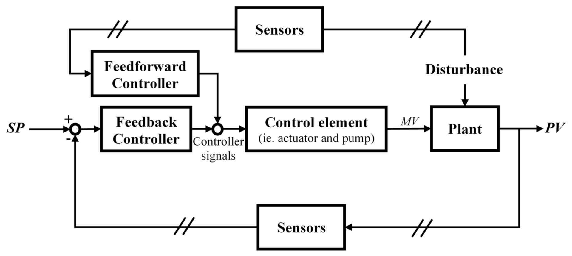
  • Feedback controller: a controller that does not act until the disturbances disrupt the process output and cause an offset from the setpoint
  • Feedforward controller: a controller that acts on measured disturbances; usually associated with feedback control to perform a cascade control that provides a more responsive, stable, and reliable control system
  • Plant/process: the process or plant model that relates the process output to the process variable and disturbance variable by a mathematical relationship
  • Sensors/transmitters: the model of equipment that generates measurements of the process output
  • Setpoint (SP): objectives of the process, typically a certain level of an output variable that is desired to maintain
  • Manipulated variable (MV): a variable that the controller can manipulate to maintain the process output as close to the setpoint as possible
  • Disturbance: variables that are meant to be constant but fluctuates or cannot be controlled; these variables can also affect the effluent quality or process efficiency
  • Output/Process variable (PV): the variable that needs to be controlled to meet environmental regulations or safety requirements
Figure 1. Structure of a typical control loop.
Environments 08 00116 g001

3. Dynamic Problems and Goals in PVA Degradation

The first step in designing process control schemes for wastewater treatment technologies is to understand the mechanisms of these processes and define their dynamic problems and goals. The knowledge of valid operational parameters can be applied to dynamic process modeling. In this section, the PVA degradation using the conventional biological treatment and AOPs are presented.

3.1. Biological Treatment of Wastewater Containing PVA

Mass production and utilization of PVA have generated a high demand for ineffective waste treatment processes that can handle large loads in a short amount of time. Biological treatment is the most conventional treatment method among all treatment methods with its major limitation in treatment times and effectiveness, dependent on microbial cultures and treatment conditions. The biodegradation of PVA can be dated back to 1936, when Fusarium line B was observed to be the first PVA-degrader, followed by Pseudomonas O-3 in 1973 [15]. Pseudomonas and Sphingomonas genus were the most well-studied microorganisms in PVA degradation [16]. In general, the biodegradation of PVA is taken care of by intracellular and extracellular degradation. Intracellular degradation initiates when PVA is engulfed into the cell’s periplasm, a space between the inner cytoplasmic membrane and the outer membrane occupied by a gel-like matrix. The PVA macromolecule is oxidized by pyrroloquinoline quinone (PQQ), a dependent PVA dehydrogenase (PVADH), with cytochrome c acting as the electron acceptor in the first step [17]. Then, the oxidized PVA (oxiPVA) is hydrolyzed by oxidized PVA hydrolase (OPH) or β-diketone hydrolase (BDH). Extracellular degradation initiates when PVA is oxidized by secreted secondary alcohol oxidase (SAO) with O2 acting as the electron acceptor. Then, the oxiPVA is hydrolyzed by secreted BDH [15,18]. However, the application of PVA-biodegradation is limited by the availability of microbial species that can generate the cofactors to PVA biodegradation: intracellular or extracellular PQQ, OPH, SAO, and BDH. Hence, most previous studies focused on the PVA-degraders isolated from activated sludge by acclimating sewage sludge with PVA being the sole substrate.
The earliest study presented by Chiellini et al. [19] conferred the relationship between PVA-degradation efficiency and microorganisms found in environments where PVA degradation took place. Low PVA film degradation (8–9%) under long treatment time (72 days) was presented by burial tests in soil not contaminated with PVA. At the same time, 13% PVA film degradation was observed after 21 days of incubation in aerobic liquid cultures inoculated with municipal sewage sludge that was not acclimated with PVA solution [19]. On the other hand, liquid cultures inoculated with paper mill sewage sludge that was previously treating paper mill wastewater containing PVA presented a much higher PVA-degradation efficiency (33.3% in 21 days and 100% in 70 days), indicating that the PVA-degradation ability of activated sludge is strictly related to the presence of PVA-degrading microorganisms that are found exclusively in environments contaminated by PVA [19].
Later studies showed the efficacy of other microorganisms in treating PVA-containing wastewater through aerobic and anaerobic treatments with acclimated microbial communities, as listed in Table 1.
Microbial phylum favored by aerobic conditions includes actinobacteria, ascomycota, bacteroidetes, chloroflexi, firmicutes, planctomycetes, proteobacteria, and other unclassified microorganisms. Chung et al. [10] achieved 98% PVA removal with a batch aerobic biodegradation by Microbacterium barkeri KCCM 10507 (phyla Actinobacteria) and Paenibacillus amylolyticus KCCM 10508 (phyla firmicutes) isolated from activated sludge from the wastewater treatment facilities in textile and dyeing factories in five days. Wei et al. [18] achieved 46.2% PVA removal with batch aerobic biodegradation by Stenotrophomonas rhizophila QL-P4 (phyla proteobacteria) isolated from fallen leaves from a virgin forest in the Qinling Mountains in five days. Magdum et al. [20] achieved 85.02% Chemical Oxygen Demand (COD) removal and 90.3% PVA removal with an optimized continuous aerobic treatment of industrial desizing effluent (0.531% PVA) using a combination of Candida Sp. (phyla Ascomycota) and Pseudomonas Sp. (phyla Proteobacteria) with two days of hydraulic retention time (HRT). Huang et al. [21] achieved 83.6% COD removal with a batch aerobic biodegradation by a mixture of phyla of PVA-degrading microorganisms in four days. Furthermore, microbial phylum favored by anaerobic conditions includes bacteroidetes, chlamydiae, firmicutes, proteobacteria, and other unclassified microorganisms. Yamatsu et al. [22] achieved 90% PVA removal with a batch anaerobic treatment using Sphingopyxis Sp. PVA3 (phyla Proteobacteria) is isolated from activated sludge in six days. Huang et al. [21] achieved 87.6% COD removal with a batch anaerobic biodegradation by a mixture of phyla of PVA-degrading microorganisms in 45 days.
Besides the importance of PVA-degrading microorganisms in the treatment system, treatment conditions and biological symbiosis also played essential roles in enhancing the PVA-degradation efficacy of a treatment system. The efficiency of PVA-biodegradation ranged differently in aerobic and anaerobic biodegradation. Aerobic biodegradation, the most commonly studied treatment process, presented efficiencies ranging from 80 to 98% PVA removal with 4 to 16 days by different inoculum. On the other hand, Anaerobic biodegradation presented a relatively high efficiency (87.6% COD removal) in a much more extended period of 45 days compared to 83.6% COD removal in four days under aerobic biodegradation while using the same sewage sludge acclimated under different conditions [21]. The microbial community in the anaerobic sludge and aerobic sludge showed apparent differences in biodiversity at the phylum levels, with Proteobacteria dominating the microbial community in both conditions. The lower pH level favors chlamydiae in anaerobic conditions. A lower abundance of some phylum and a higher abundance of chlamydiae and bacteroidetes were presented under anaerobic conditions rather than aerobic conditions [21]. Aerobic and anaerobic conditions also showed a significant difference in class level of proteobacteria phyla, with alphaproteobacteria dominating in aerobic conditions and betaproteobacteria dominating in anaerobic conditions. Overall, aerobic treatment was more efficient than anaerobic treatment due to a higher abundance of alphaproteobacteria as the dominant enzymatic PVA-mineralizing bacteria [21,23]. Hence, the difference in the efficacy of the processes was due to the difference in the abundance of microbial classes and phylum changes according to their growth conditions.
Likewise, differences in operating conditions under the same operation scheme (anaerobic or aerobic) would lead to differences in biodegradation efficiencies. Magdum et al. [20] achieved 85.02% COD removal and 90.3% PVA removal with an optimized continuous aerobic treatment of industrial desizing effluent (0.531% PVA) using a combination of Candida Sp. (phyla ascomycota) and Pseudomonas Sp. (phyla proteobacteria) with two days of HRT while controlling air flowrate to prevent foaming of the solution. Candida Sp. and Pseudomonas Sp. inoculation was carried out in five days with a 2% PVA solution as the sole source of the nutrient. Treatment conditions such as aeration rate and stirring rate played an important role in biodegradation efficacy where higher aeration presented foaming, and lower aeration presented slower biodegradation rate. Concurrently, the lower stirring rate presented a slower biodegradation rate, while the higher and optimized stirring rate presented similar efficacy. The optimized aeration rate and stirring rate were found at 16 L/min and 150 rpm, respectively.
Moreover, Vaclavkova et al. [24] studied the symbiosis factor of Sphingomonas Sp. OT3, previously proven to be an efficient PVA-degrader, experiments in cultures amended with PQQ and active or inactive catalase [17]. With the essential cofactor in PQQ put aside, S. OT3 presented low PVA degradation (28% in 30 days) without the presence of inactive catalase (82% in 30 days with S. OT3 + inactive catalase) and Rhodococcus erythropolis OT3 (88% in 30 days with S. OT3 + R. erythropolis OT3) when no enzyme activities were detected in the culture media, indicating the absence of extracellular enzyme secretion [24]. It was most likely that the PVA macromolecule could not cross the outer membrane of S. OT3 due to its chemical structure. On the other hand, P. erythropolis OT3 helped to cleave PVA by PVA oxidase and a possible hydrolase or lyase on the outer membrane to smaller fragments capable of crossing the outer membrane of S. OT3 [17]. The PVA degradation process was followed by further PVA oxidation by PQQ in the periplasm of S. OT3. Similarly, the results from a study conducted by Bian et al. [6] also indicated a substantial limitation of PVA-degradation efficiency related to the ability of the PVA macromolecule to migrate through the cell membrane. This migration occurred as the PVA-degradation efficiency increased from 10 to 68.5% in batch experiments using Bacillus niacini screened from sludge samples and cross-linked enzyme aggregates (CLEAs) of PVA degrading enzymes (PVAase) from Bacillus niacin, respectively.
Overall, PVA-biodegradation using different microbial communities was valid under circumstances that the PVA-degraders and cofactors are present and well-controlled. However, PVA-degrading microorganisms are not commonly found in the current ecosystem, and bacteria isolated from a previously contaminated setting by PVA are not commonly present in the uncontaminated environment. PVA biodegradation presented high reliance on the capability of PVA macromolecules to cross the outer membrane of microbial cells. Hence, PVA-biodegradation generates a high demand for specific acclimated microbial populations to achieve significant biodegradation. PVA-biodegradation is also accompanied by excessive sludge production [5,20]. Withal, even in a setting where PVA-degrading bacteria are present, the biological treatment process is slow and intractable compared to physicochemical processes and AOPs due to possible excessive sludge generation.
Table 1. Biological treatments of PVA-containing wastewater.
Treatment Systems and Microbial CulturesTarget PollutantsTreatment TimesOptimal Experimental ConditionsResultsRef.
Soil and liquid cultures inoculated with municipal sewage sludgePVA-based blown films74 dDegradation in soil8–9% PVA removalChiellini et al. [19]
21 dDegradation in liquid cultures inoculated with municipal sewage sludge13% PVA removal
70 dDegradation in liquid cultures inoculated with paper mill sewage sludge100% PVA removal
Batch treatment using Sphingopyxis Sp. PVA3Aqueous PVA+ pyrroloquinoline quinone (PQQ)6 d[PVA]i = 1 g/L, 30 °C, stirring rate = 120 rpm90% PVA removalYamatsu et al. [22]
Batch treatment using Sphingomonas Sp. OT3 and Phodococcus erythropolis OT3 Aqueous PVA + PQQ30 d-88% PVA degradation by S. OT3 and P. erythropolis OT3Vaclavkova et al. [24]
Continuous treatment using Candida Sp. and Pseudomonas Sp.Industrial desizing effluent containing PVA2 d[PVA]i = 5.19 g/L, [COD]i = 14,861 mg/L, O2 flowrate = 16 L/min, stirring rate = 150 rpm85.02% COD and 90.3% PVA removalsMagdum et al. [20]
Batch treatment using Microbacterium barkeri KCCM 10507 and Paenibacillus amylolyticus KCCM 10508Aqueous PVA5 d[PVA]I = 950 mg/L, [COD]I = 2250 mg/L, suspended solids = 1400 mg/L, pH 7, 30 °C98% PVA removalChung et al. [10]
Anaerobic-aerobic bioreactor with PVA-degrading microorganismsAqueous PVA45 d in anaerobic and 4 d in aerobic[PVA]i = 3 g/L, 40 °C (anaerobic), 25 °C (aerobic), DO = 2 mg/L87.6 and 83.6% COD removals in anaerobic and aerobic stagesHuang et al. [21]
Batch treatment using two PVA-degrading Sphingomonas strainsAqueous PVA16 d[PVA]i = 0.5 g/L, suspended solids = 300,000 cells/100 mL, 25 °C80% PVA removalMěrková et al. [25]
Batch treatment using Stenotrophomonas rhizophila QL-P4Aqueous PVA5 d[PVA]i = 1.0 g/L46.2% PVA removalWei et al. [18]
Batch treatment using cross-linked enzyme aggregates (CLEAs) of PVA degrading enzymes (PVAase) from Bacillus niaciniAqueous PVA3 h[PVA]i = 1 g/L, [(NH4)2SO4]i = 70%, [C5H8O2]i = 1.50%, crosslinking time = 1 h, pH 7, 40 °C68.5% PVA removalBian et al. [6]

3.2. Treatment of Aqueous PVA by AOPs

Unlike biological treatment methods, AOPs are a series of robust wastewater treatment processes dependent on highly reactive free radicals, particularly hydroxyl and hydroperoxyl radicals (HO and HO2), and radical intermediates accompanied with high efficiencies in a relatively short treatment time [5,26]. AOPs can degrade carbonaceous compounds to intermediates, such as carboxylic acids, and fully oxidized forms (CO2 and H2O) in a much shorter period than biological degradation processes [3]. Many intermediates formed during AOPs are more readily biodegradable if not fully degraded as compared to parent compounds. Although AOPs present high efficacy in the degradation of carbonaceous compounds, they are expensive for industrial applications and are coupled with high technicalities requirements. Previous applications of AOPs in the treatment of PVA-containing wastewater are summarized in this section, including electrochemical and photoelectrochemical oxidation, Fenton and photo-Fenton oxidation, ionizing radiation (IR), ozonation, persulfate oxidation, photocatalytic oxidation, ultrasound cavitation, UV-hydrogen peroxide oxidation (UV/H2O2), and wet air oxidation. These processes are classified into chemical-based AOPs, energy-based AOPs, and hybrid AOPs, as listed in Table 2, Table 3 and Table 4.

3.2.1. Fenton-Based Processes: Fenton/Photo-Fenton/Electro-Fenton

Fenton-based processes are commonly applied in industrial wastewater treatment to aid the treatment of organic recalcitrant that the conventional biological treatment processes cannot treat. Although Fenton-based oxidation pre-treatment processes, with a relatively short HRT before an activated sludge process, help meet the required effluent qualities, the fluctuation in Fenton-based processes’ effluent quality related to the influent properties remains the primary concern. The Fenton process consists of a set of well-known reactions between hydrogen peroxide (H2O2) and iron metal (Fe2+) to degrade a polymeric pollutant (Pr) are as follows:
H 2 O 2 + Fe 2 + Fe 3 + + HO + HO H 2 O 2 + Fe 3 + Fe OOH 2 + + H + Fe OOH 2 + Fe 2 + + HO 2 HO 2 + H 2 O 2 O 2 + H 2 O + HO P r + HO HO + P r P r + Fe 3 + P r + + Fe 2 + P r + + H 2 O P r OH + H +
The degradation of PVA pollutant (Pr) by hydroxyl radicals formed in the Fenton reactions would generate intermediates with lower molecular weights, such as alcohols, aldehydes, ketones, and acids [28,30],
P r + HO h v intermediates CO 2 + H 2 O .
Besides, ferric coagulation plays a significant role in removing PVA in the Fenton process [28,31]. According to previous studies, the decolorization of wastewater was mainly contributed by Fenton oxidation under acidic conditions (pH 2–5), and the removal of COD was mainly contributed by iron coagulation under neutral to basic conditions (pH 6–10) [27,28]. Additionally, there is an optimum H2O2 dosage along with Fe2+ dosage for Fenton-based processes; this optimum dosage can differ from one treatment system to another based on the concentration of the pollutant in the system [27,29,32]. The efficiency of Fenton-based processes could also be affected by purging gas [29,32], PVA molecular weight [32,33], temperature [27,32], and scavenging effect of other organic pollutants present in the treatment system [27,28].
The photochemically enhanced Fenton processes (UV/Fe2⁺/H₂O₂) studied by Bossmann et al. [32,33], Giroto et al. [8], Kang et al. [31], and Lei et al. [30] present higher COD/Dissolved Oxygen Demand (DOC) reduction than Fenton, which is most likely due to the enhanced reduction efficiency of iron (III) to iron (II) and the formation of hydroxyl radicals through photolysis of hydrogen peroxide under irradiation by the following reactions,
Fe 3 + + H 2 O h v Fe 2 + + H + + HO H 2 O 2 h v HO
Similar to Fenton oxidation, the hydroxyl radicals should participate in the oxidation of organic molecules into their intermediates. However, there was no evidence for forming hydroxyl radicals as reactive intermediates and generating low molecular weight PVA intermediates (oxalic acid, acetic acid, acetaldehyde, ethanol, or PVA-oligomers) in the photo-Fenton process [32]. In contrast, results from gel permeation chromatography present experimental evidence for the formation of a super macromolecule of iron (III)-oxidized PVA complexes exhibiting a molecular weight (100,000 g/mol) much higher than that of PVA (15,000, 49,000, and 100,000 g/mol), which could proceed Fenton-type oxidation, accompanied by ferryl-ion (Fe4+(aq)) formed within the complex, directly releasing CO2 from the complex [33]. Meanwhile, a heterogeneous photo-Fenton process using the iron (III)-exchanged zeolite Y catalyst, instead of iron (II), presented lower DOC reduction. Nevertheless, Bossmann et al. [33] found evidence in the formation of low molecular weight intermediates (step-by-step degradation of PVA molecules) and the absence of super macromolecule confirming that iron (III) remains bounded within the zeolite Y framework.

3.2.2. Ozonation

With the development of industrial-scale ozone generators and the implementation of ozonation water/wastewater treatment systems, ozone (O3) has drawn increasing attention in treating wastewater containing refractory organic pollutants in various concentrations. Ozonation is efficient in degrading organic compounds and fully oxidizing its intermediates owing to its powerful oxidizing capability. It is also friendly to most organisms as it would not introduce other substances into the treated wastewater. The ozonation process undergoes different pathways under acidic and basic conditions. Under acidic conditions (pH < 4), the ozone molecule is stable, and it would directly react with pollutants with specific functional groups through dipolar addition reactions, nucleophilic reactions, or electrophilic reactions. Since the affinity of an oxygen atom is very high, the oxidative potential of ozone under acidic conditions is also high. Under basic conditions (pH > 9), the ozone molecule is less stable, and it could interact with other reactants in the following reactions to form oxidative hydroxyl radicals:
O 3 + OH HO 2 + O 2 O 2 + O 3 O 3 + O 2 O 3 + H + HO 3 HO 3 HO + O 2
where O3 and HO both play essential roles in oxidizing the organic pollutant (PVA) to intermediates with lower molecular weights, as shown in the following reaction:
P r + O 3 intermediates CO 2 + H 2 O
The degradation of PVA to formic acid and other carboxylic acids during ozonation was experimentally proven by the pH shift of the medium towards acidic conditions [35]. In contrast to Fenton oxidation, the foaming ability of PVA could trap ozone into the PVA molecules competing with the oxidation of PVA molecules and intermediates with lower molecular weights, such as alcohols, aldehydes, ketones, and acids [35]. Previous studies presented that ozone is more efficient under alkaline conditions [34]. However, higher efficiency can be obtained using microbubble technology to enhance the yield of hydroxyl radicals [36].

3.2.3. UV/Hydrogen Peroxide Oxidation (UV/H2O2)

The hydrogen peroxide oxidation mechanism is constructed by two reactions: photolytic reactions of hydrogen peroxide and PVA degradation. The photolytic reactions of hydrogen peroxide produce oxidative radicals ( HO and HO 2 ) that are critical players in PVA degradation as shown below [39,53,54,55,56,57,58,59]:
Initiation: H 2 O 2 h v 2 HO
Propagation: HO + H 2 O 2 HO 2 + H 2 O
H 2 O 2 + HO 2 HO + H 2 O + O 2
HO + HO 2 HO 2 + OH
O 2 + H + HO 2
HO 2 O 2 + H +
Termination: HO + HO H 2 O 2
HO 2 + HO H 2 O + O 2
HO 2 + HO 2 H 2 O 2 + O 2
HO 2 + O 2 O 2 + HO 2
HO + O 2 O 2 + OH
Electron transfer: HO 2 + H + H 2 O 2
H 2 O 2 HO 2 + H +
The degradation kinetics of UV/H2O2 in the treatment of PVA-containing wastewater was first modeled by Hamad et al. (2018), where an overview of the degradation process is as follows:
P r + H 2 O 2 h v intermediates CO 2 + H 2 O .
The polymer degrades from r number of chains to PVA with r-s number of chains, carboxylic acids, dimers, and monomers. These degradation and mineralization reactions take place simultaneously in the reactors as follows [3]:
Initiation: H 2 O 2 hv 2 HO
P n hv P n n 2
Propagation: P n + HO P n + H 2 O
P n + HO 2 P n + H 2 O 2
P n + HO P n a + P a
P n + HO P n 1 + P 1
P 1 + 2 HO + 5 2 O 2 2 HCOOH + 2 HO 2
P 1 + HO 2 CH 3 COOH + HO
HO + CH 3 COO C H 2 COO + H 2
Termination: P 1 + HO 2 + O 2 2 HCOOH + OH
CH 3 COOH + 2 HO 2 2 HCOOH + H 2 O 2
HCOOH + 2 HO CO 2 + 2 H 2 O
Electron transfer: CH 3 COOH CHO 3 COOH + H +
HCOOH CH 3 COO + H +
HCOO + H 2 O 2 CO 2 + H 2 O + OH
The formation of intermediates was proven by gel permeation chromatography analyses, which presented a decrease in average molecular weight of pollutants existing in the aqueous system and a decrease in pH, representing the formation of acidic intermediates throughout the batch reaction [3,60]. The PVA degradation efficiency was found to be favored by acidic conditions (pH 3) when compared with neutral and alkaline conditions (pH 7 and 11) [37]. More importantly, there is an interaction effect on pollutant removal, molecular weight reduction, and H2O2 residual, between H2O2 dosage and influent PVA concentration, which presented an optimal H2O2-to-PVA mass ratio of 1.0 at the influent stream [61,62].

3.2.4. Persulfate Oxidation

Persulfate (S2O82) is another molecule with high oxidative potential when excited under UV irradiation, the addition of transition metal ions (Mn+ such as Ag+, Co2+, Fe2+), or heat to generate sulfate radicals ( SO 4 ) as explained by the following reactions:
S 2 O 8 2 h e a t / h v 2 SO 4 S 2 O 8 2 + M n + SO 4 + M n + 1 + SO 4 2
where the generation of SO 4 is favored by acidic conditions [37,41]. Then, the sulfate radicals could form highly oxidative hydroxyl radicals via the following reactions,
SO 4 + H 2 O HO + H + + SO 4 2   under   all   pH SO 4 + OH HO + SO 4 2   under   alkaline   pH .
Hydroxyl radicals and sulfate radicals would participate in the oxidation of pollutants (PVA) to form intermediates with lower molecular weights. Previous studies found that hydroxyl radicals ( HO ) react very poorly with PVA in persulfate oxidation under alkaline conditions, where the efficiency of PVA degradation was reduced when the sulfate radicals ( SO 4 ) are scavenged by hydroxide ions ( OH ) to form hydroxyl radicals ( HO ), making hydroxyl radicals the dominant oxidative species [37,41]. Hence, persulfate oxidation performs better under acidic conditions. For the polymer, the degradation reaction is as follows:
P r + SO 4 intermediates + SO 4 CO 2 + H 2 O + SO 4 2 .
The formation of intermediates was experimentally proven by mass spectroscopy of PVA solution oxidized by persulfate oxidation [40]. However, during excitation with a transition metal, an excessive amount of transition metal, such as iron (Fe2+), might scavenge sulfate radicals [7,40] as shown below:
S 2 O 8 2 + Fe 2 + SO 4 + Fe 3 + + SO 4 2 Fe 2 + + SO 4 Fe 3 + + SO 4 2
The scavenging reaction competes with the formation of hydroxyl radicals. Also, excessive sulfate radicals might scavenge persulfate molecules under saturated sulfate radical concentrations [41],
SO 4 + S 2 O 8 2 SO 4 2 + S 2 O 8
Most importantly, persulfate oxidation efficiency increased with increasing persulfate dosage in the UV excited system but is optimum when it is excited using a transition metal (Fe2+).

3.2.5. Photocatalytic Oxidation

In wastewater treatment, photocatalytic oxidation by titanium dioxide (TiO2) has been commonly studied because it is low in cost, highly efficient, biologically and chemically inert, resistant to photo corrosion, and non-toxic [63,64]. It has evolved from ultraviolet (UV) photooxidation to visible light photooxidation by modifying the properties of the photocatalyst. Traditionally, titanium dioxide is activated by UV to generate hydroxyl radicals by the following reaction mechanisms,
TiO 2 hv h vb + + e cb
where photogenerated electrons participate in,
O 2 ads + e cb O 2 ads O 2 ads + H + HO 2 2 HO 2 O 2 + H 2 O 2 H 2 O 2 + O 2 ads HO + OH + O 2
and photogenerated holes participate in,
HO ads + h vb + HO
H 2 O ads + h vb + HO + H + .
The generated by-products react together to form more hydrogen peroxide that participates in the previous reaction mechanisms,
2 O 2 + 2 H 2 O O 2 + H 2 O 2 + 2 OH .
The degradation mechanism is affected by UV dosage, TiO2 dosage, pH, temperature, and initial PVA concentration [42,63,64,65]. Also, PVA degradation is more efficient under higher UV dosage, and higher temperatures as both conditions enhance the reaction rate by providing more energy to the system. Also, PVA degradation is more efficient under acidic or alkaline pH as both conditions promote HO generation from photogenerated electrons and holes, respectively. The TiO2 dosage was optimal at 2 g/L [42]. Lower TiO2 dosage leads to lower hydroxyl radical generation, and a higher TiO2 dosage leads to turbidity, which reduces UV transmission.
Some studies suggest that its efficiency could be enhanced by adding hydrogen peroxide to increase the generation of hydroxyl radicals, as shown in the following reactions:
H 2 O 2 h v 2 HO H 2 O 2 ads + e cb HO + HO H 2 O ads + h vb + HO + H + O 2 + H 2 O 2 OH + HO + O 2 .
However, excess H2O2 will scavenge HO and lead to lower PVA degradation. The degradation of PVA follows a similar degradation mechanism as shown in the peroxide oxidation of PVA,
P r + HO intermediates CO 2 + H 2 O
Although photocatalytic oxidation processes are efficient and reliable, the separation of the photocatalyst in suspension form is problematic. The efficiency of the immobilized photocatalyst is much lower than the suspended form owing to the reduction in available reaction surface.

3.2.6. Wet Air Oxidation

Wet air oxidation (WAO) is an AOP performed in the aqueous phase under elevated temperature and high pressure, with the presence of oxygen or air, where the pollutant (PVA) is broken down by oxygen to form oxidative species, as demonstrated in the following reaction:
P r + O 2 P r + H O 2 2 P r + O 2 P r + H 2 O 2 H 2 O 2 HO
The reaction kinetic is significantly affected by the temperature, where higher temperatures presented higher degradation efficiency [43,44,45]. When hydrogen peroxide is added to the WAO process, it promotes wet air oxidation (PWAO). If oxygen is replaced by hydrogen peroxide, the process becomes wet peroxide oxidation (WPO). Then, the polymer radical is degraded in the same fashion as shown in the peroxide oxidation method to smaller polymer segments, organic acids, other intermediates, and finally to fully oxidized forms (CO2 and H2O). This degradation pathway is supported by forming formic acid and acetic acid throughout the treatment process and increasing biodegradability of PVA-wastewater through the expansion of reaction time such that the intermediates formed are much more biodegradable than PVA itself [43,45]. Between WAO and PWAO, PWAO presented higher degradation efficiency in a shorter time [44]. However, excess hydrogen peroxide, especially in the WPO process, can result in a scavenging effect leading to lower PVA degradation efficiency [44]. Moreover, excess in oxygen (200% excess oxygen ratio) at a constant oxygen partial pressure and acidic conditions (pH 2.5) favors the degradation of PVA [44,45].

3.2.7. Electrochemical-Based Oxidation

The electrochemical oxidation process utilizes an electrical current to generate oxidative and reductive species in the system. Electrochemical oxidation of recalcitrant can occur directly at the anodes or indirectly. Direct electrochemical-based oxidation is initiated by anodic reactions to produce surface adsorbed hydroxyl radicals and chemisorbed active oxygen at the surface metal oxide lattice (M) [5,66], as shown below:
M + H 2 O M HO ads + H + + e M HO   ads MO + H + + e M HO ads M + 1 / 2   O 2 + H + + e MO 1 / 2   O 2 + M
The direct oxidation of pollutant (PVA) happens at the surface of the anode [66], as shown in the following:
P r + M HO   ads m CO 2 + n H 2 O + H + + e P r + MO RO + M
As the duration of the electrolysis increases, indirect oxidation of PVA begins as the reaction between the by-products (e, H+, and O2) from the anodic reaction at the cathode proceeds to generate hydrogen peroxide (H2O2) [4], as follows:
O 2 + 2 H + + 2 e H 2 O 2
However, higher current density induces the decomposition of hydrogen peroxide:
H 2 O 2 + 2 e 2 OH H 2 O 2 HO 2 + H + + 2 HO 2 O 2 + H + + e .
On top of that, the electrochemical-based treatment is favored by acidic conditions (pH = 3) owing to the generation of the oxonium ion (H3O22+) that enhances the stability of hydrogen peroxide molecules [4]:
H 2 O 2 + H + H 3 O 3 + .
At the same time, the reduction of hydrogen peroxide and hydrogen gas production takes place at the cathode,
H 2 O 2 + 2 H + + 2 e 2 H 2 O 2 H + + 2 e H 2 .
Hence, the efficiency of electrochemical oxidation can be drastically improved using photo-energy (UV irradiation), known as photoelectrochemical oxidation, as it activates the electrogenerated H2O2 to form hydroxyl radicals, which can oxidize organic pollutants (PVA) by hydrogen peroxide oxidation reactions [4]. Moreover, photoelectrochemical oxidation can be enhanced by adding transitional metals Men+ as both the photogenerated hydroxyl radicals and an excited transition metal, Men+1, participate in the degradation of PVA molecules at the anode and cathode, respectively. The transition metal is excited at the cathode [47],
Ce 3 + Ce 4 + + e P r + Ce 4 + intermediates CO 2 + H 2 O .

3.2.8. Ionizing Radiation (IR) (Electron Beam Radiation and ϒ Radiation)

Ionizing radiation is a unique AOP that includes two types of radiations, electron beam radiation, and gamma-ray (ϒ) radiation, to generate oxidative species, H2O2 and HO, and reducing species, H and eaq [49,50,52], as shown in the following reaction under pH 7:
H 2 O r a d i a t i o n 2.8 HO + 2.7 e a q + 0.6 H + 0.7 H 2 O 2 + 0.45 H 2 + 3.2 H a q + + 0.5 O H a q
This reaction was found to be sensitive to pH [49,50], dissolved gases [49], presence of radical scavengers [49,50,52], added hydrogen peroxide dosage [49,50], and radiation dose rate [48,49,51,52] along with the interaction between different pairs of factors.
The pH of the system mainly controls the recombination of reductive species. Under acidic conditions, the reductive specie eaq formed will react with free H+ to form the other reductive specie H, as shown below:
e aq + H + H
In contrast, under basic conditions, the reaction is between H and free OH to form eaq as follows:
H + HO e aq
Under excess of dissolved oxygen, the reductive species formed will recombine to oxidative peroxyl radicals, HO2, and O2, as shown in the following:
H + O 2 HO 2 e aq + O 2 O 2
At the same time, other solvents, such as isopropyl alcohol ( CH 3 CHOHCH 3 ) and tert-butyl alcohol ( CH 3 3 COH ), scavenge hydrogen radical and hydroxyl radical to form intermediates [50,52], based on the following reactions:
CH 3 CHOHCH 3 +   HO CH 2 C OHCH 3 + H 2 O CH 3 CHOHCH 3 +   H CH 2 C OHCH 3 + H 2 CH 3 3 COH +   HO C H 2 C CH 3 2 OH + H 2 O CH 3 3 COH +   H C H 2 C CH 3 2 OH + H 2
The pollutant (PVA) degradation is similar to that of peroxide oxidation mechanisms, as shown previously. Under pH 6.8, oxygen gas saturated systems performed better with the addition of isopropyl alcohol, which contributed to 3.07% PVA degradation, and nitrogen gas saturated systems performed better with tert-butyl alcohol, contributing to 7.65% PVA degradation [49]. However, both systems presented the highest efficiency under the absence of scavenger species under the same pH, indicating a robust scavenging effect from the added solvents.
Meanwhile, hydrogen peroxide is generated in the system and can be added to the system. It undergoes a different reaction mechanism to generate oxidative species, as shown in the following reactions:
H 2 O 2 + e aq HO + OH H 2 O 2 + H H 2 O + HO H 2 O 2 + HO H 2 O + HO 2
The addition of hydrogen peroxide can increase the number of oxidative hydroxyl radicals generated in the system, further increasing the chance of degraded PVA by hydroxyl radicals. However, excess hydrogen peroxide would lead to the scavenging effect on the hydroxyl radicals. The scavenging reaction is undesirable as the excess hydrogen peroxide would compete with PVA molecules and inhibit its degradation. Overall, ionizing radiation technologies presented sound PVA degradation and improvement in Biological Oxygen Demand (BOD) to the COD ratio of the wastewater. On top of that, strong interactions between radiation dose rate and initial PVA concentration, hydrogen peroxide, and pH could have different effects on PVA degradation depending on the pair of factors [50].

4. Process Identification: Process, Disturbance, and Control Variables

Generally, PVA-wastewater treatment technologies are associated with different manipulated, disturbance, and process variables depending on their applicability. These variables cannot accept any value; they are constrained by technical limitations and environmental and safety standards. The automation of wastewater treatment faced many problems, mainly in the lack of information regarding the processes to be controlled. Prior knowledge is the basic building block of process models. Table 3 presents a list of manipulated variables, disturbances, and process variables that apply to PVA-wastewater-treatment technologies. This review article does not cover all types of modeling and controller design techniques because the scope of this review article is to summarize models and controllers feasible, applicable to PVA degradation in wastewater treatment. Therefore, this section covers control-oriented process models and process control strategies applied to wastewater treatment technologies discussed in previous sections. A summary of previous studies is presented in Table 4. Other modeling methods and process control strategies not covered in this article, like fuzzy neural network modeling, adaptive control, and neural network control, display themselves as research gaps in the study of process control in wastewater treatment processes.
Table 3. List of Manipulated variables, disturbances, and process variables in the PVA degradation process.
TypeExamples
Manipulated variableOperational conditions:
aeration rate/intensity
dilution rate
recycle ratio in biological treatments
dosages of reactants, such as Fe2+, O3, H2O2, S2O82−, O2, which can be controlled by dosing method or flowrate in AOPs
energy input such as electric current density, radiation dosage, and irradiation dosage in AOPs
Process output variables:
oxidation-reduction potential (ORP)
oxygen transfer coefficient,
pH, to estimate process outputs that cannot be measured on-line
DisturbanceInfluent quality:
  • influent PVA concentration
  • TOC
  • COD
  • BOD
  • TN
  • TP
  • pH
Operational conditions:
  • temperature
  • pressure
  • other equipment specifications
  • flowrate, which also controls the reaction time
  • dosage of reactants that are kept constant
Process variableEffluent quality:
  • PVA concentration
  • TOC
  • COD
  • BOD
  • TN
  • TP
  • TSS
  • ammonia
  • nitrate nitrogen
  • pH
  • residual H2O2
Process efficiencies:
  • color removal
  • COD removal
  • effluent absorbance
Operating conditions:
  • DO for biological processes
  • concentrations of excess reactants for AOPs
Recent studies on control-oriented process identification methods have become increasingly popular due to the effectiveness of model-based control strategies in achieving superior system performance in setpoint tracking and load disturbance rejection for various industrial processes. In set-point tracking, the controller acts on the input of a set-point by selecting its actions on the control element to manipulate the process variable to reach the desired set-point value. In disturbance rejection, the controller acts on a deviation caused by a disturbance by forcing the process variable back to the desired setpoint.

4.1. Mechanistic vs. Data-Driven System Identification

Mechanistic models are usually utilized to obtain dynamic models and parameters of a thoroughly known process with known parameters and their effect on the process, such as biological processes in wastewater treatment [67]. Mechanistic models could be developed from fundamental principles of chemical, physical, and biochemical processes. However, mechanical modeling of wastewater treatment processes is associated with first-principles modeling accompanied by complex reaction mechanisms and intense computation; it is usually used to design wastewater treatment plant (WWTP) processes and is rarely employed in dynamic models. In dynamic modeling, system identification (SI) is usually utilized to build dynamic black-box models based on input/output data using linear regression methods and parameters of imprecisely known processes. The variables in a black box model are determined from previous knowledge of measurable factors exploited by the state or parameters of the system. Among all methods, a step test in an open-loop structure of the linear parameter varying (LPV) process is usually practiced given its economical and straightforward implementation with applications toward a wastewater treatment process. This method can accomplish multivariate parameter estimation under appropriate constraints using the maximum likelihood approach. LPV modeling implies performing a parameter estimation by minimizing the sum of squares of error between the observed output and model-predicted output during step tests initiated at the zero-initial or other states of a process moving towards the desired operating region [68,69].

4.2. Static vs. Dynamic Modeling of Pollutant Removal

Chemical processes can be modeled by two types of states: static and dynamic. Each modeling method is accompanied by its advantages and trade-offs. Static modeling, also known as steady-state modeling, seeks to optimize operational conditions during steady-state operation [70]. These types of system outputs depend only on the present values of the inputs. Hence, it is a lofty design and a set of operating conditions that are not consistently maintained due to chemical processes’ dynamic behavior. In a dynamic process, steady-state models can express the effect of different factors onto process efficiencies using algebraic equations and, most importantly, the static objectives of a process known as the setpoints [12,70]. Contradictory, dynamic modeling seeks to study the dynamic, transient behavior of chemical processes. It considers transient influent qualities and operational conditions on process efficiencies through mechanistic and black box modeling methods. These models are usually described by differential or difference equations, and their outputs are dependent on present and past values of inputs. Thus, dynamic modeling is more suitable for designing process control models. Black-box modeling is preferred between the two dynamic modeling methods when mechanistic modeling is sophisticated, hard to solve, and when its solution requires extensive computation [68].

5. Dynamic Behavior of Wastewater Treatment Processes

The first step to designing a process control system is to establish a process model. Dynamic process models can be built on prior knowledge of general laws and principles (mechanistic models) and experimental input and output data (black box models). Dynamic process models can also be built to study dynamics in batch or continuous processes. As mechanisms describing wastewater treatment processes are complex, the system identification method is commonly applied to build models relating a process output to input via black-box modeling. During modeling, a system is linear when a change in all parameters is always the sum of their individual effects. A system is nonlinear when an input signal is correlated to another input signal. Thus, wastewater treatment processes are nonlinear. When the process is slightly nonlinear, it may be sufficient to approximate it with a linear transfer function and implement linear control. If the nonlinearity is strong, it is more appropriate to consider the system nonlinearity in the process model and the controller design. Since most wastewater treatment processes are associated with nonlinearity and process dead time, incorporating nonlinearity estimators is necessary to describe the system adequately. These dynamic models can be developed using mechanistic, system identification, and artificial intelligence models (artificial neural networks and support vector regression). This section focuses on dynamic models that have been applied to wastewater treatment technologies discussed in previous sections.

5.1. State-Space Model

State-space models are mechanistic models that use state variables or parameters to describe a system using first-order differential or difference equations. This class of models is a great starting choice for a quick estimation of the dynamic relationship between the input/output dataset. It only requires one specification, the model order. The model order is the dimension of the state variable related to the number of delayed inputs and outputs used in the state-space model. The measurable factors of a process are exploited by states or parameter estimators through a state-space model in continuous time as follows:
d x d t = A x + B u
with process output given by:
y = C x + D u  
where A, B, C, and D are matrices containing the characteristic parameters of the system, u is a vector of system inputs, and x is the state vector of the system. In discrete-time modeling, the state-space is written in a different form as follows:
x k t k + t k = A x k t k + B u k t k
y k t k = C x k t k + D u k t k .
where the sample number k is taken at sampling interval tk since wastewater treatment processes are nonlinear, a more general model for wastewater treatment processes is as follows:
d x d t = f x , u , t k t k , θ
y = g x , t k t k , θ
The relationship between process input and output, state variables, and model parameters (θ) is described by nonlinear functions f and g.
The state variables can be obtained by mechanistic modeling [67], system identification parameter estimation [71,72,73,74,75,76], or just system identification parameter estimation [77,78,79,80]. Pure mechanistic state-space modeling is applicable only in cases where the mechanism of the system is thoroughly known, such as an activated sludge process [67]. However, parameter estimation using the mechanistic state-space model requires more substantial computation than using system identification. Simultaneously, mechanistic state-space modeling, accompanied by system identification parameter estimation, can better represent the existing treatment system. It estimates state variables using actual input/output data despite theoretical estimation in mechanistic modeling for well-known processes prone to disturbances in operational conditions, such as biological treatment processes [72,73,74,75,76] and photo-Fenton processes [71]. On the other hand, state-space modeling of complex systems with unknown model orders is usually accomplished through the system identification method. State-space models with different model orders can be identified and compared to determine the best model order. Therefore, there is no “best solution” to the process model for processes that are not thoroughly understood; the state-space modeling technique would depend on the availability of knowledge on the treatment processes.

5.2. Transfer Function Model

A transfer function model is the ratio of polynomials used to describe the relationship between inputs and outputs of a system. Similar to the state-space models, transfer function models can also be in continuous-time or discrete-time forms. Dynamic models based on Laplace transfer functions are used to describe continuous systems, whereas dynamic models describe discrete systems based on z-transformed transfer functions. In the past, both system identification models had been the “go-to” model during black-box modeling owing to their simplicity and applicability to PI/PID controller design [81,82,83]. The continuous transfer function Gp(s) relating the output signal y(s) to the input signal u(s) is as follows [81,84]:
G p s = y s u s = K b m s m + b m 1 s m 1 + + b 1 s + 1 a n s n + a n 1 s n 1 + + a 1 s + a 0 e d s  
where y(s) and u(s) are the Laplace transform of the signals y(t) and u(t), K is the process gain, an and bm are coefficients, d is the time-delay (process dead time), m is the number of zeros, and n is the number of poles (order) of the transfer function with nm for realizable systems. The unknown coefficients, a and b, are estimated by the least-squares method. Dynamic process modeling commonly uses first-order and second-order transfer functions plus time-delay (FOPTD and SOPTD).
Alternatively, for a sampled-data system, discrete transfer functions require the transformation of the output variable y(t) and input variable u(t) by z-transform as follows:
y t = y k t k
u t = u k t k
where k is the sample number, and tk is the sampling interval. The discrete process model that describes the dependency of system output y(nk) on past and present system inputs (u(nk)) at nkth sample obtained at a constant sampling interval of tk in a single-input single-output (SISO) system is known as AutoRegressive model with eXogenous input (ARX) [85] written as follows:
A z 1 y k = z d B z 1 u k 1 + e k  
where z 1 is the backward shift operator, d is the delay in the system, and e n k is the stochastic disturbance. The polynomials of   A z 1 and B z 1 are of nth and mth order given in forms of:
A z 1 = 1 + a 1 z 1 + a 2 z 2 + + a n z n  
B z 1 = b 0 + b 1 z 1 + b 2 z 2 + + b m z m
where model parameters are a1, a2, …, an and b0, b1, …, and bn. The estimation of the process model utilizes the linear-time-varying-regression as follows:
y ^ k , θ ^ = Φ T k θ ^ k
where θ ^ k is the unknown parameter vector as shown below:
θ ^ k = a 1 a 2           a n b 0 b 1   b m
while Φ k is the regression vector containing past values of u(k) and y(k), as shown below:
Φ T = y k 1 y k 2   y k n u k d 1 u k d 2   u k d m 1
Similarly, the unknown parameters are estimated by the least-squares method.
The unknown parameter coefficients ( θ ^ k ) are estimated by the maximum likelihood method, where the error between the predicted output and the measured output is minimized. Continuous process models had been applied to the model ozonation process [81], photo-Fenton process [82], photocatalytic oxidation process [83], as well as full-scale wastewater treatment plants [84]. On the other hand, discrete process models had been applied to model activated sludge processes [85]. These process models can precisely model and predict process dynamics of continuous-flow systems with a more straightforward model form, a lower model order, and a smaller dataset. However, since process output signals are usually sampled at time intervals, it is more suitable to model treatment processes with a discrete model. These discrete signals can later be transformed into a continuous signal using an Analog-to-Digital converter, which adds a zero-order hold to compute continuous process signals if the sampling time is within the Nyquist frequency. Overall, both models presented excellent system stability, high fitness to the actual output values, and applicability to feedback controller design.

5.3. Artificial Neural Networks

Artificial neural networks (ANNs) are supervised artificial intelligence machine learning models broadly employed for prediction, classification, and optimization purposes in data-driven process modeling due to their ability to capture nonlinear behavior between inputs and outputs [86,87,88,89,90,91]. Generally, an ANN is a network of simple nonlinear process units known as neurons. These neurons are arranged and interconnected in a network structure with a specific number of layers consisting of an input layer, specified numbers of hidden layers (minimum of one), and an output layer. Each connection between ith neuron in the previous layer and the jth neuron in the current layer is assigned with a specific weight (wij). Each neuron has an independent bias (bj) input. The neuron output (yj) is determined from an activation function (f) built on the sum of its inputs (xi) and independent bias using a back-propagation (BP) algorithm, also known as the back-propagation neural network (BPNN), as written in the following equation:
y j = f b i + i = 1 n x i w i j .  
The maximum of i and j, known as K and Q, are the number of neurons in the preceding and the number of outputs in the current hidden layer. The resulting value is then sent to the next layer and processed by another transfer function (f) in the network, where this procedure is repeated until the output layer. The standard BP algorithm is based on the gradient search, which moves network weight and threshold backward along the performance function gradient while minimizing errors between actual and predicted output values [13].
A radial basis function neural network (RBFNN) is another type of NN based on radial basis functions (RBF) as activation functions in the neurons [92,93,94,95]. It identifies as a superior ANN model because it can map principles with a higher tolerance of input noises and online learning on a larger dataset [95]. RBFNN consists of an input layer, a Gaussian RBF layer, and a linear output layer. The Gaussian RBF layer is made of neurons with Gaussian transfer functions with outputs θk(x(t)) as written in the following equation:
θ k x t = exp x t μ k t σ k 2  
where μk is the center vector of the kth hidden neuron, σk2 is the radius or width of the kth hidden neuron, and the denominator is the Euclidean distance between the input of the network x and μk at time t. Thus, the linear output layer obtains process output y by:
y t = k = 1 M w k θ k x t  
where wk is the weight between the kth hidden neuron and the output neuron.
Both types of ANN have been applied for soft-sensor to their flexible structure of nonlinear neurons, universal approximation, and efficient generalization performance [87]. Supervised NN using BPNN has been used to predict: treatment efficacy of Fenton [90], photo-Fenton [87], and Electro-Fenton processes [89]; treatment efficacy of UV/H2O2 process [88]; and effluent quality of WAO [96]. Supervised NN using RBF has been used to predict dissolved oxygen (DO) concentration in a biological treatment process [92]. Although the ANN is usually employed to compute more massive datasets, it demonstrated promising prediction accuracy even when small input–output datasets are available [87]. Additionally, the ANN presented the ability to approximate off-line measurements dynamically, resulting in savings in off-line sampling and analyses.

6. Controller Algorithms

In general, the goal of a control system is to maintain a process output close to the desired value by managing the inputs using control elements. These control elements can be electric, pneumatic, or electromechanical actuators. Process control can be categorized into linear control and linearizing control. Linear control deals with systems modeled in continuous or discrete forms, which are the most common methods in automatic control. Most wastewater treatment systems are controlled by conventional linear controllers [12]. Linearizing control deals with non-linearity in the process models through different strategies and control algorithms depending on the application. Linearization control is usually accomplished by linearizing the nonlinear process model during controller design. This section discusses the applicability and advantages of different controllers in wastewater treatment technologies.

6.1. PID Control

Proportional integral derivative (PID) controller and its variants, proportional (P) and proportional-integral (PI) controllers, are the conventional linear controller commonly employed in wastewater treatment processes [12]. These controllers apply corrections to the manipulated variable by comparing the real-time measured and desired signals. A PID controller is suitable when the control system is well-defined with a stable characteristic and is modeled in a continuous-time signal as follows:
G c s = K c 1 + K I s + K D s T f  
and in a discrete-time signal in the following form:
G c s = K c 1 + K I I F z + K D T f + D F z  
where Kc, KI, and KD are the controller, integral, and derivative gains, respectively. The controller, integral, and derivative gains are the tuning parameters of PID controllers. The term Tf refers to the first-order derivative filter time constant, and IF(z) and DF(z) are the discrete integrator formulas for the integrator and derivative filters as shown below:
I F z = D F z = T s z 1
where Ts is the sampling time.
PI and PID controllers are designed for single-variant linear transfer function models and tuned with an identified dynamic process model. PI and PID controllers have been applied to control effluent quality in ozonation processes [97], photo-Fenton processes [82,98], and photocatalysis oxidation [83]. Although wastewater treatment processes are nonlinear, it is possible to maintain proper set-point tracking and disturbance rejection using PI and PID controllers in lightly nonlinear processes by approximating the process with a linear process model [82]. However, the performance of P, PI, and PID controllers degrades when significant process nonlinearities are associated with disturbances in a control system and when there is a lack of state variables that can be measured during operation [12,13]. Therefore, an adaptive controller is required to estimate the various parameters of the process during each control interval using an algorithm that can predict process efficiencies based on state variables measured during operation.

6.2. Model Predictive Control

In contrast to linear PID control, model predictive control (MPC) is an advanced control strategy that addresses nonlinearities via linearization to achieve optimal control and adaptive control. Traditionally, MPC uses mechanistic dynamic process models to predict a process over time intervals, prediction horizons, and variables while accounting for process variables’ physical constraints. Two types of predictive control, MPC and nonlinear MPC (NMPD), have been used to model wastewater treatment systems dynamically. The NMPC is an MPC that is solved using a nonlinear process model. The MPC determines the present and future controller action (Δuk, Δuk+1, …, Δuk+Nu−1) by minimizing the cost function J written as follows:
J N 1 , N 2 , N u = j = N 1 N 2 Γ y ^ t + j | t y r e f + j | t 2 + j = 1 N u Λ Δ u t + j 1 2
where y ^ t + j | t , y r e f + j | t , and Δ u t + j 1 are the predicted outputs along the prediction horizon, the reference signal, and the control effort over the control horizon of N u , respectively. The predicted output is computed using linear/nonlinear process models such as ARX, state-space, NARX, and NN. The tuning parameters in the cost function are the prediction horizons ( N 1 and N 2 ), control horizon N u , and input-output coefficient weights ( Λ and Γ ). The difference between the minimum prediction horizon and maximum prediction horizon, which are represented by N 1 and N 2 , is the time range where the future output must follow the reference signal. The selection of these tuning parameters is determined through process settling time and computational limitations. The minimum prediction horizon is usually more significant than the process dead time ( d ), and the weight matrix Γ is an identity matrix for a SISO process. In most cases, the weight matrix Λ (ny × nu) is set to Λ = λ I , where λ is the scalar weighting coefficient, I = Ψ , and Ψ is a square diagonal scaling matrix (ny × nu).
MPC is uncommon in WWTPs as most individual processes, such as biological processes and AOPs, are too complex to develop sufficiently accurate mechanistic models based on first principles due to disturbances that cause processes to deviate from ideal operational conditions. However, many have investigated the applicability of system identification models to MPC design. The cost function of MPC can be solved analytically by approximating a linear process model for a system that is only lightly nonlinear with no constraints on inputs or outputs; this linear process model can range from linear state-space models [75,80] to linear system identification models [99]. The generalized predictive control (GPC) is another type of linear feedback MPC. Sadeghassadi et al. [85] proposed a constrained GPC and a PI control that uses the oxygen transfer coefficient to control DO concentration in the last tank. The constrained GPC has an inequality constraint on a controlled variable based on the physical limits of the equipment. The GPC showed better and smoother set-point tracking and disturbance rejection for constrained GPC than PI control, lower mean squared error (MSE), and lower squared input-step-change (||∆u||2).
Moreover, Stare et al. [75], Santín et al. [80], and Liu and Yoo [99] were able to achieve good set-point (DO, effluent ammonium, and effluent nitrate) tracking and disturbance (variations in flowrate) rejection when approximating WWTPs with discrete linear transfer function models. However, MPC based on nonlinear process models performed better than MPC based on linear process models because most wastewater treatment processes are nonlinear [75]. The cost function of MPC for nonlinear process models, known as NMPC, can only be solved using linearization of nonlinear process models [72,100] or iterative optimization algorithms [78,92] for MPC to achieve excellent setpoint tracking of nonlinear processes. The solution of the NMPC scheme is mathematically and computationally intense, making it not easy to implement WWTP processes. Even though several studies tried to implement MPC onto WWTP processes, more research is required to develop system-specific models before MPC can be implemented in full-scale WWTPs. Moreover, the MPC is unsuitable for WWTP processes because MPC real-time control is restricted by possible inaccuracy in identified dynamic models.
Table 4. Dynamic process model and process control strategies of wastewater treatment technologies.
Target PollutantProcess and Controller ModelsProcess Inputs: Manipulated Variables and DisturbancesProcess Output:
Process Variable
ResultsRef.
Activated sludge processes
Primary sewage effluentTime-series process modelsInfluent volatile organic compound (VOC) concentrationsEffluent VOC concentrationsNo apparent effect of solid retention time or hydraulic retention time on VOC removalMelcer et al. [101]
Actual wastewaterMechanistic state modelAeration rate
Dilution rate
Recycled ratio
DOShowed successful simulated state model based on the state variable sensibilitiesCaraman et al. [67]
Actual wastewaterMPC design based on nonlinear reduced-order and linear, mechanistic state modelDO in first and second aerobic reactors
Influent ammonia
Temperature
Influent flowrate
Effluent ammoniaShowed relatively large MRSE errors in model prediction
MPC showed the ability to correct deviations resulted from deficiencies in the process model
MPC with nonlinear state model performed better than MPC with the linear state model
Stare et al. [75]
Actual wastewaterIntegrated design for MPC on the mechanistic state modelInternal recycle flowrateNitrate level in the anoxic tankMPC showed optimal controlFrancisco et al. [72]
Actual wastewaterNMPC-PI control based on the nonlinear mechanistic state modelAirflow rateTotal suspended solids (TSS)
Wastewater flowrate
Effluent ammonia
Set-point tracking achieved
NMPC-PI controller showed better performance than centralized NMPC
Francisco et al. [78]
Actual wastewaterGPC and PI design based on ARX process modelOxygen transfer coefficient
Influent flow rate
Influent concentration
DOGPC showed high robustness to disturbances
GPC performed better than conventional PI control
Sadeghassadi et al. [85]
Actual wastewaterMPC based on the mechanistic state modelExternal carbon flow rate
Internal recirculation flow rate
Nitrate nitrogen in tank 5
Nitrate nitrogen in influent
MPC simulation showed improvement in process efficiencySantín et al. [80]
Actual wastewaterNMPC based on self-organizing (SR) RBF NN process modelInternal recycle flow rate
Oxygen transfer coefficients in the fifth aerated reactor
Dissolved oxygen (DO)SR-RBF NN model showed high fitness to measured data
SR-RBF-NMPC showed good control ability and reduced tracking errors of DO even under high disturbances
Han et al. [92]
Actual wastewaterMPC design based on the mechanistic state modelFlow rate
Influent substrate concentration
Dilution rate
DOMPC simulation showed good setpoint control and disturbance rejectionHarja et al. [74]
Actual wastewaterCascade control with two PI single-variant controllers and a multi-variant MPC based on a fifth-order MIMO modelExternal carbon flowrateEffluent nitrate concentration
Effluent ammonium concentration
Nitrate concentration in the second reactor1
DO in the last reactor1
Process model showed high fitness (>88.9%) to measured data
Successful control of effluent nitrate level
Liu and Yoo [99]
Sequencing batch reactor
Actual wastewaterSISO non-linear mechanistic state modelValve openingDO
Respiration rate
Oxygen transfer coefficient
Simulation showed promising estimation of process outputsHvala et al. [79]
Wastewater treatment plant (WWTP)
Industrial coke wastewaterClosed-loop feedback controller based on SOPTD process modelAirflow rateDOReduced SOPTD model showed a good representation of the real plant and robust ability to measurement noise and step disturbancesYoo and Kim [84]
Actual wastewaterMPC based on a state-space modelFlowrate
Recycle flowrate
Aeration intensity
Buffer tank holdup
Effluent ammonium
Fluent nitrate
MPC presented good controllability of the process even under unpredicted disturbancesElixmann et al. [77]
Actual wastewaterNonlinear mechanistic state-space modelFlowrateEffluent ammoniumSuccessful estimation of model parametersGašperin et al. [73]
Actual wastewaterMPC based on a steady-state process modelFlow rate
Influent ammonia
Influent pH
Effluent COD
Effluent phosphorous (TP)
Steady-state models showed high fitness (81.6% and 77.2%)
MPC showed good controllability
Wang et al. [76]
Fenton
Pigment wastewaterFeedback process control based on multiple regressionH2O2 dosage
Oxidation-reduction potential (ORP)
Influent COD
Effluent CODModels showed higher fitness to measured data
Control system was effective in maintaining stable effluent quality
Kim et al. [86]
Textile wastewaterSingle variable ANN-BPNN process modelORP
pH
Fe2+ dosage
Color removal
COD removal
No direct or linear correlation between color/COD removal efficiencies and ORP and pH in the oxidation tank
Color/COD removal BPN model showed high fitness to experimental results
Yu et al. [90]
Photo-Fenton
WastewaterPI control with an anti-windup mechanism based on SOPTD grey-box process modelPercentage of H2O2 pump frequency output[H2O2]PI controller showed good set-point tracking with high robustness in small-scale and pilot-scale tests
Alvarez et al. [82]
ParacetamolPI control with an anti-windup mechanism based on FOPTD process modelH2O2 dosage
Pollutant concentration
UV radiation
DOFOPTD showed high fitness to the measured output
PI controller showed good set-point tracking and disturbance rejection with high robustness
Ortega-Gómez et al. [98]
ParacetamolMathematical state modelIlluminated volume to total volume ratio (Ri)DO
[TOC]
[H2O2]
Model showed high fitness to experimental results
Effect of Ri was significant and possible to use for scale-up
Cabrera Reina et al. [71]
ParacetamolData-driven ANN process modelH2O2 dosage
Initial TOC
Effluent TOCModel presented high approximation ability of final TOC (RMSE = 0.73–2.81)Shokry et al. [87]
Electro-Fenton
Textile wastewater
(not dynamic modeling)
ANN-BPNN modelORP
Reaction time for ORP to reach the ORP valley
Reaction time for DO rising point
Desired COD removal
Fe2+ dosage
Fe2+ requirement
Actual COD removal
ORP and DO profiles showed the ability to indicate the variations in [H2O2], [Fe2+], and [Fe3+]
ANN model demonstrated more precise predictions results than regression models
Yu et al. [89]
Peroxide oxidation (UV/H₂O₂)
Azo dye
(not dynamic modeling)
ANN-BPNN model with ten neurons in the hidden layerNozzle angle (θN)
Nozzle diameter (dN)
Flow rate (Q)
Initial concentration of H₂O₂
pH
Reaction time (t)-
Process efficiency measured by UV absorbanceBPNN model showed high fitness with the order of importance for variation of variables as [H2O2]0 > t > pH > Q > θN > dNSoleymani et al. [88]
Ozonation
Paranitrophenol aqueous solutionContinuous-time transfer function model with delayO3 generator powerEffluent absorbance
Ozone gas concentration at the top of the reactor
Model showed high fitness in identification data (90.3%) and validation data (86.2%)Abouzlam et al. [81]
Secondary effluent from municipal WWTPPID controller based on the time-series process modelO3 dosageChange in UV absorbance at 254 nm (ΔUV254) between effluent and influent measurement
Closed-loop process controller presented good set-point tracking
Linear regression fitted well between ΔUV254 and TOC removal (%)
Stapf et al. [97]
Electrochemical oxidation
Phenolic compoundsTen steps ahead prediction based on stacked NN modelsCurrent density
Pollutant concentration
pH
Temperature
Phenolic compound type
Chlorine compound type
Effluent CODStacked NN model with two hidden layers presented the highest fit, the average relative error of 1.75%, and R2 of 0.9998 against the training dataset
Stacked NN model also presented good accuracy with prediction errors (4–6%) against the validation dataset
Piuleac et al. [102]
Photocatalytic oxidation
ToluenePI feedback and feedforward controllers based on FOPTD process modelIllumination intensity of the LED light source
Inlet toluene concentration
Relative humidity
Toluene conversion (%) Feedback controller presented proper set-point tracking and the ability to mitigate catalyst deactivation
Feedforward controller based on the empirical steady-state model presented excellent disturbance rejection
Khodadadian et al. [83]
Wet air oxidation
Phenolic compoundsANN-BPNN model with three layersWeighted hourly space velocity (WHSV)
pH
Temperature
Pressure
Time
Phenol conversion (%)NN model presented high fitness and low errorGheni et al. [96]

7. Conclusions and Recommendations

In this study, different wastewater treatment processes available for PVA degradation were explained in detail. Although it is possible to acclimate biological treatments to achieve PVA degradation in existing WWTPs, the degradation process in biological treatment processes is very slow. On the other hand, the degradation process in AOPs is non-selective and faster than biological processes, but they still require more research to develop fundamental mechanisms. Among all, UV/H2O2 remains a popular process for degrading and mineralizing PVA in the wastewater system through photoreaction owing to its non-selective degradation kinetics, low cost, and ease of operation. Meanwhile, the industrial application of AOPs requires future control strategies to maintain process efficiencies, effluent qualities, and process reliability under variable operational conditions while preventing system failure. Despite numerous counts in WWTP process control literature, there is no “best” approach on the road for process control. Control-oriented process models for an existing treatment can be built on mechanistic and system identification models using historical monitoring data. The latter approach is much simpler than the earlier approach as mechanistic models of wastewater treatment processes are complex and computationally intense.
Control-oriented models can be used to design PI/PID controllers and predictive controllers, depending on system requirements. PI/PID controllers are more common and thoroughly understood between the two, so their implementation would be much more straightforward than predictive controllers. Plus, the weakness of PI/PID controllers in linearization control can be easily overcome using adaptive control. In contrast, more research is required to develop a system-specific solution before MPC can be implemented in full-scale processes. Moreover, MPC cannot be applied to all WWTP processes simply because its real-time control is limited by the number of online measurable inputs and outputs and inaccuracy in model predictions.
In summary, wastewater treatment technologies looking to integrate controllers should:
  • Define the scope and the desired goals of the treatment processes.
  • Identify process variables that can be used as manipulated variables (variables that can be changed to move the process towards the desired set-point), control variables (variables that need to be constrained), and disturbances (variables that cannot be controlled but have effects on process efficiency or effluent quality).
  • For automation of existing processes, use plotting tools to visualize the effect of each process variable via plotting monitoring data. For automation of new processes, design and perform step testing experiments to obtain process data and visualize the effect of each process variable via plotting monitoring data.
  • Identify a suitable control strategy based on the observed data or experimental data trends and desired goals.
  • Fit and validate process models that are suitable for the identifies control strategy. The choice for a dynamic model would depend on the size of the dataset, the number of variables to be studied, and the nonlinearity of the processes.
  • Design and validate the control strategy based on the identified dynamic process model.
  • Implement and validate control design.

Author Contributions

Writing—original draft preparation, Y.-P.L.; Writing—review and editing, R.D. and M.M.; Supervision, R.D. and M.M. All authors have read and agreed to the published version of the manuscript.

Funding

This research was funded by Natural Sciences and Engineering Research Council of Canada (NSERC) and Ryerson University Faculty of Engineering and Architectural Science Dean’s Research Fund.

Institutional Review Board Statement

Not applicable.

Informed Consent Statement

Not applicable.

Data Availability Statement

Not applicable.

Acknowledgments

We: the authors, greatly appreciate the financial support of the Natural Sciences and Engineering Research Council of Canada (NSERC) and Ryerson University Faculty of Engineering and Architectural Science Dean’s Research Fund.

Conflicts of Interest

The authors declare no conflict of interest.

References

  1. Swift, G. Requirements for Biodegradable Water-Soluble Polymers. Requir. Biodegrad. Water-Soluble Polym. 1997, 59, 19–24. [Google Scholar] [CrossRef]
  2. Swift, G. Environmentally Biodegradable Water-Soluble Polymers. In Degradable Polymers, 2nd ed.; Scott, G., Ed.; Springer: Dordrecht, The Netherlands, 2002; pp. 379–412. [Google Scholar]
  3. Hamad, D.; Mehrvar, M.; Dhib, R. Photochemical Kinetic Modeling of Degradation of Aqueous Polyvinyl Alcohol in a UV/H2O2 Photoreactor. J. Polym. Environ. 2018, 26, 3283–3293. [Google Scholar] [CrossRef]
  4. Huang, K.Y.; Wang, C.T.; Chou, W.L.; Shu, C.M. Removal of Polyvinyl Alcohol Using Photoelectrochemical Oxidation Processes Based on Hydrogen Peroxide Electrogeneration. Int. J. Photoenergy 2013, 2013, 841762. [Google Scholar] [CrossRef]
  5. Sun, W.; Chen, L.; Wang, J. Degradation of PVA (Polyvinyl Alcohol) in Wastewater by Advanced Oxidation Processes. J. Adv. Oxid. Technol. 2017, 20. [Google Scholar] [CrossRef]
  6. Bian, H.; Cao, M.; Wen, H.; Tan, Z.; Jia, S.; Cui, J. Biodegradation of Polyvinyl Alcohol Using Cross-Linked Enzyme Aggregates of Degrading Enzymes from Bacillus Niacini. Int. J. Biol. Macromol. 2019, 124, 10–16. [Google Scholar] [CrossRef] [PubMed]
  7. Dong, Y.; Bian, L.; Wang, P. Accelerated Degradation of Polyvinyl Alcohol via a Novel and Cost Effective Heterogeneous System Based on Na2S2O8 Activated by Fe Complex Functionalized Waste PAN Fiber and Visible LED Irradiation. Chem. Eng. J. 2019, 358, 1489–1498. [Google Scholar] [CrossRef]
  8. Giroto, J.A.; Guardani, R.; Teixeira, A.C.S.C.; Nascimento, C.A.O. Study on the Photo-Fenton Degradation of Polyvinyl Alcohol in Aqueous Solution. Chem. Eng. Process. Process Intensif. 2006, 45, 523–532. [Google Scholar] [CrossRef]
  9. Samal, K.; Maiti, K.; Mohanty, K.; Das, C. Ultrafiltration of Aqueous PVA Using Spinning Basket Membrane Module. Water. Air. Soil Pollut. 2018, 229. [Google Scholar] [CrossRef]
  10. Chung, J.; Kim, S.; Choi, K.; Kim, J.O. Degradation of Polyvinyl Alcohol in Textile Waste Water by Microbacterium Barkeri KCCM 10507 and Paenibacillus Amylolyticus KCCM 10508. Environ. Technol. 2016, 37, 452–458. [Google Scholar] [CrossRef]
  11. Sun, W.; Chen, L.; Zhang, Y.; Wang, J. Synergistic Effect of Ozonation and Ionizing Radiation for PVA Decomposition. J. Environ. Sci. 2015, 34, 63–67. [Google Scholar] [CrossRef] [PubMed]
  12. Iratni, A.; Chang, N.B. Advances in Control Technologies for Wastewater Treatment Processes: Status, Challenges, and Perspectives. IEEECAA J. Autom. Sin. 2019, 6, 337–363. [Google Scholar] [CrossRef]
  13. Newhart, K.B.; Holloway, R.W.; Hering, A.S.; Cath, T.Y. Data-Driven Performance Analyses of Wastewater Treatment Plants: A Review. Water Res. 2019, 157, 498–513. [Google Scholar] [CrossRef] [PubMed]
  14. Vanrolleghem, P.A.; Lee, D.S. On-Line Monitoring Equipment for Wastewater Treatment Processes: State of the Art. Water Sci. Technol. 2003, 47, 1–34. [Google Scholar] [CrossRef]
  15. Ben Halima, N. Poly(Vinyl Alcohol): Review of Its Promising Applications and Insights into Biodegradation. RSC Adv. 2016, 6, 39823–39832. [Google Scholar] [CrossRef]
  16. Klomklang, W. Biochemical and Molecular Characterization of a Periplasmic Hydrolase for Oxidized Polyvinyl Alcohol from Sphingomonas Sp. Strain 113P3. Microbiology 2005, 151, 1255–1262. [Google Scholar] [CrossRef]
  17. Kawai, F. Sphingomonads Involved in the Biodegradation of Xenobiotic Polymers. J. Ind. Microbiol. Biotechnol. 1999, 23, 400–407. [Google Scholar] [CrossRef] [PubMed]
  18. Wei, Y.; Fu, J.; Wu, J.; Jia, X.; Zhou, Y.; Li, C.; Dong, M.; Wang, S.; Zhang, J.; Chen, F. Bioinformatics Analysis and Characterization of Highly Efficient Polyvinyl Alcohol (PVA)-Degrading Enzymes from the Novel PVA Degrader Stenotrophomonas Rhizophila QL-P4. Appl. Environ. Microbiol. 2017, 84. [Google Scholar] [CrossRef] [Green Version]
  19. Chiellini, E.; Corti, A.; D’Antone, S.; Solaro, R. Biodegradation of PVA-Based Formulations. Macromol. Symp. 1999, 144, 127–139. [Google Scholar] [CrossRef]
  20. Magdum, S.S.; Minde, G.P.; Adhyapak, U.S.; Kalyanraman, V. An Efficient Biotreatment Process for Polyvinyl Alcohol Containing Textile Wastewater. Water Pract. Technol. 2013, 8, 469–478. [Google Scholar] [CrossRef]
  21. Huang, J.; Yang, S.; Zhang, S. Performance and Diversity of Polyvinyl Alcohol-Degrading Bacteria under Aerobic and Anaerobic Conditions. Biotechnol. Lett. 2016, 38, 1875–1880. [Google Scholar] [CrossRef] [PubMed]
  22. Yamatsu, A.; Matsumi, R.; Atomi, H.; Imanaka, T. Isolation and Characterization of a Novel Poly(Vinyl Alcohol)-Degrading Bacterium, Sphingopyxis Sp. PVA3. Appl. Microbiol. Biotechnol. 2006, 72, 804–811. [Google Scholar] [CrossRef] [PubMed]
  23. Pathak, V.M. Navneet Review on the Current Status of Polymer Degradation: A Microbial Approach. Bioresour. Bioprocess. 2017, 4. [Google Scholar] [CrossRef]
  24. Vaclavkova, T.; Ruzicka, J.; Julinova, M.; Vicha, R.; Koutny, M. Novel Aspects of Symbiotic (Polyvinyl Alcohol) Biodegradation. Appl. Microbiol. Biotechnol. 2007, 76, 911–917. [Google Scholar] [CrossRef] [PubMed]
  25. Měrková, M.; Julinová, M.; Houser, J.; Růžička, J. An Effect of Salt Concentration and Inoculum Size on Poly(Vinyl Alcohol) Utilization by Two Sphingomonas Strains. J. Polym. Environ. 2018, 26, 2227–2233. [Google Scholar] [CrossRef]
  26. Larking, D.M.; Crawford, R.J.; Christie, G.B.Y.; Lonergan, G.T. Enhanced Degradation of Polyvinyl Alcohol by Pycnoporus Cinnabarinus after Pretreatment with Fenton’s Reagent. Appl. Environ. Microbiol. 1999, 65, 1798–1800. [Google Scholar] [CrossRef] [Green Version]
  27. Lin, S.H.; Lo, C.C. Fenton process for treatment of desizing wastewater. Water Res. 1997, 31, 7. [Google Scholar] [CrossRef]
  28. Bae, W.; Won, H.; Hwang, B.; de Toledo, R.A.; Chung, J.; Kwon, K.; Shim, H. Characterization of Refractory Matters in Dyeing Wastewater during a Full-Scale Fenton Process Following Pure-Oxygen Activated Sludge Treatment. J. Hazard. Mater. 2015, 287, 421–428. [Google Scholar] [CrossRef]
  29. Lin, C.C.; Hsu, S.T. Performance of NZVI/H 2 O 2 Process in Degrading Polyvinyl Alcohol in Aqueous Solutions. Sep. Purif. Technol. 2018, 203, 111–116. [Google Scholar] [CrossRef]
  30. Lei, L.; Hu, X.; Yue, P.L.; Bossmann, S.H.; Gob, S.; Braun, A.M. Oxidative Degradation of Poly Vinyl Alcohol by the Photochemically Enhanced Fenton Reaction. J. Photochem. Photobiol. Chem. 1998, 116, 159–166. [Google Scholar] [CrossRef]
  31. Kang, S.F.; Liao, C.H.; Po, S.T. Decolorization of Textile Wastewater by Photo-Fenton Oxidation Technology. Chemosphere 2000, 41, 1287–1294. [Google Scholar] [CrossRef]
  32. Bossmann, S.H.; Oliveros, E.; Göb, S.; Kantor, M.; Göppert, A.; Braun, A.M.; Lei, L.; Yue, P.L. Oxidative Degradation of Polyvinyl Alcohol by the Photochemically Enhanced Fenton Reaction. Evidence for the Formation of Super-Macromolecules. Prog. React. Kinet. Mech. 2001, 26, 113–137. [Google Scholar] [CrossRef]
  33. Bossmann, S.H.; Oliveros, E.; Göb, S.; Kantor, M.; Göppert, A.; Lei, L.; Yue, P.L.; Braun, A.M. Degradation of Polyvinyl Alcohol (PVA) by Homogeneous and Heterogeneous Photocatalysis Applied to the Photochemically Enhanced Fenton Reaction. Water Sci. Technol. 2001, 44, 257–262. [Google Scholar] [CrossRef]
  34. Shin, H.S.; Yoo, K.S.; Kwon, J.C.; Lee, C.Y. Degradation Mechanism of PVA and HEC by Ozonation. Environ. Technol. 1999, 20, 325–330. [Google Scholar] [CrossRef]
  35. Cataldo, F.; Angelini, G. Some Aspects of the Ozone Degradation of Poly(Vinyl Alcohol). Polym. Degrad. Stab. 2006, 91, 2793–2800. [Google Scholar] [CrossRef]
  36. Takahashi, M.; Chiba, K.; Li, P. Free-Radical Generation from Collapsing Microbubbles in the Absence of a Dynamic Stimulus. J. Phys. Chem. B 2007, 111, 1343–1347. [Google Scholar] [CrossRef]
  37. Lin, C.C.; Lee, L.T. Degradation of Polyvinyl Alcohol in Aqueous Solutions Using UV/Oxidant Process. J. Ind. Eng. Chem. 2015, 21, 569–574. [Google Scholar] [CrossRef]
  38. Hamad, D.; Mehrvar, M.; Dhib, R. Experimental Study of Polyvinyl Alcohol Degradation in Aqueous Solution by UV/H2O2 Process. Polym. Degrad. Stab. 2014, 103, 75–82. [Google Scholar] [CrossRef]
  39. Hamad, D.; Dhib, R.; Mehrvar, M. Effects of Hydrogen Peroxide Feeding Strategies on the Photochemical Degradation of Polyvinyl Alcohol. Environ. Technol. 2016, 37, 2731–2742. [Google Scholar] [CrossRef] [PubMed]
  40. Oh, S.Y.; Kim, H.W.; Park, J.M.; Park, H.S.; Yoon, C. Oxidation of Polyvinyl Alcohol by Persulfate Activated with Heat, Fe2+, and Zero-Valent Iron. J. Hazard. Mater. 2009, 168, 346–351. [Google Scholar] [CrossRef] [PubMed]
  41. Lin, C.C.; Lee, L.T.; Hsu, L.J. Degradation of Polyvinyl Alcohol in Aqueous Solutions Using UV-365 Nm/S2O8 2−Process. Int. J. Environ. Sci. Technol. 2014, 11, 831–838. [Google Scholar] [CrossRef] [Green Version]
  42. Chen, Y.; Sun, Z.; Yang, Y.; Ke, Q. Heterogeneous Photocatalytic Oxidation of Polyvinyl Alcohol in Water. J. Photochem. Photobiol. Chem. 2001, 142, 85–89. [Google Scholar] [CrossRef]
  43. Chen, G.; Lei, L.; Yue, P.L.; Cen, P. Treatment of Desizing Wastewater Containing Poly(Vinyl Alcohol) by Wet Air Oxidation. Ind. Eng. Chem. Res. 2000, 39, 1193–1197. [Google Scholar] [CrossRef]
  44. Lei, L.; Wang, D. Wet Oxidation of PVA-Containing Desizing Wastewater. Chin. J. Chem. Eng. 2000, 8, 52–56. [Google Scholar]
  45. Won, Y.S.; Baek, S.O.; Tavakoli, J. Wet Oxidation of Aqueous Polyvinyl Alcohol Solution. Ind. Eng. Chem. Res. 2001, 40, 60–66. [Google Scholar] [CrossRef]
  46. Kim, S.; Kim, T.H.; Park, C.; Shin, E.B. Electrochemical Oxidation of Polyvinyl Alcohol Using a RuO2/Ti Anode. Desalination 2003, 155, 49–57. [Google Scholar] [CrossRef]
  47. Huang, K.Y.; Wang, C.T.; Chou, W.L.; Shu, C.M. Removal of Polyvinyl Alcohol in Aqueous Solutions Using an Innovative Paired Photoelectrochemical Oxidative System in a Divided Electrochemical Cell. Int. J. Photoenergy 2015, 2015, 623492. [Google Scholar] [CrossRef]
  48. Deogaonkar, S.C.; Wakode, P.; Rawat, K.P. Electron Beam Irradiation Post Treatment for Degradation of Non Biodegradable Contaminants in Textile Wastewater. Radiat. Phys. Chem. 2019, 165, 108377. [Google Scholar] [CrossRef]
  49. Zhang, S.J.; Yu, H.Q. Radiation-Induced Degradation of Polyvinyl Alcohol in Aqueous Solutions. Water Res. 2004, 38, 309–316. [Google Scholar] [CrossRef]
  50. Zhang, S.J.; Yu, H.Q.; Ge, X.W.; Zhu, R.F. Optimization of Radiolytic Degradation of Poly(Vinyl Alcohol). Ind. Eng. Chem. Res. 2005, 44, 1995–2001. [Google Scholar] [CrossRef]
  51. Jo, H.J.; Lee, S.M.; Kim, H.J.; Kim, J.G.; Choi, J.S.; Park, Y.K.; Jung, J. Improvement of Biodegradability of Industrial Wastewaters by Radiation Treatment. J. Radioanal. Nucl. Chem. 2006, 268, 145–150. [Google Scholar] [CrossRef]
  52. Sun, W.; Tian, J.; Chen, L.; He, S.; Wang, J. Improvement of Biodegradability of PVA-Containing Wastewater by Ionizing Radiation Pretreatment. Environ. Sci. Pollut. Res. 2012, 19, 3178–3184. [Google Scholar] [CrossRef]
  53. Bielski, B.H.J.; Cabelli, D.E. Highlights of Current Research Involving Superoxide and Perhydroxyl Radicals in Aqueous Solutions. Int. J. Radiat. Biol. 1991, 59, 291–319. [Google Scholar] [CrossRef]
  54. Buxton, G.V.; Greenstock, C.L.; Helman, W.P.; Ross, A.B. Critical Review of Rate Constants for Reactions of Hydrated Electrons, Hydrogen Atoms and Hydroxyl Radicals (⋅OH/⋅O in Aqueous Solution. J. Phys. Chem. Ref. Data 1988, 17, 513–886. [Google Scholar] [CrossRef] [Green Version]
  55. Crittenden, J.C.; Hu, S.; Hand, D.W.; Green, S. A Kinetic Model For H2O2/UV Process in a Completely Mixed Batch Reactor. WATER Res. 1999, 33, 2315–2328. [Google Scholar] [CrossRef]
  56. Elliot, A.J.; Buxton, G. Temperature Dependence of the Reactions OH + O2 and OH + HO2 in Water up to 200 °C. J. Chem. Soc. Faraday Trans. 1992, 88, 6. [Google Scholar] [CrossRef]
  57. Ghafoori, S.; Mehrvar, M.; Chan, P.K. Photoreactor Scale-up for Degradation of Aqueous Poly(Vinyl Alcohol) Using UV/H2O2 Process. Chem. Eng. J. 2014, 245, 133–142. [Google Scholar] [CrossRef]
  58. Liao, C.H.; Gurol, M.D. Chemical Oxidation by Photolytic Decomposition of Hydrogen Peroxide. Environ. Sci. Technol. 1995, 29, 3007–3014. [Google Scholar] [CrossRef]
  59. Weinstein, J.; Bielski, B.H.J. Kinetics of the Interaction of Perhydroxyl and Superoxide Radicals with Hydrogen Peroxide. The Haber-Weiss Reaction. J. Am. Chem. Soc. 1979, 101, 58–62. [Google Scholar] [CrossRef]
  60. Hamad, D.; Mehrvar, M.; Dhib, R. Kinetic Modeling of Photodegradation of Water-Soluble Polymers in Batch Photochemical Reactor. In Kinetic Modeling for Environmental Systems; Abdel Rahman, R.O., Ed.; IntechOpen: London, UK, 2019; ISBN 978-1-78984-726-0. [Google Scholar]
  61. Hamad, D. Experimental Investigation of Polyvinyl Alcohol Degradation in UV/H2O2 Photochemical Reactors Using Different Hydrogen Peroxide Feeding Strategies. Ph.D. Thesis, Ryerson University, Toronto, ON, Canada, 2015. [Google Scholar]
  62. Hamad, D.; Dhib, R.; Mehrvar, M. Photochemical Degradation of Aqueous Polyvinyl Alcohol in a Continuous UV/H2O2 Process: Experimental and Statistical Analysis. J. Polym. Environ. 2016, 24, 72–83. [Google Scholar] [CrossRef]
  63. Lin, Y.; Mehrvar, M. Photocatalytic Treatment of An Actual Confectionery Wastewater Using Ag/TiO2/Fe2O3: Optimization of Photocatalytic Reactions Using Surface Response Methodology. Catalysts 2018, 8, 409. [Google Scholar] [CrossRef] [Green Version]
  64. Nasirian, M.; Lin, Y.P.; Bustillo-Lecompte, C.F.; Mehrvar, M. Enhancement of Photocatalytic Activity of Titanium Dioxide Using Non-Metal Doping Methods under Visible Light: A Review. Int. J. Environ. Sci. Technol. 2018, 15, 2009–2032. [Google Scholar] [CrossRef]
  65. Nasirian, M.; Bustillo-Lecompte, C.F.; Lin, Y.P.; Mehrvar, M. Optimization of the Photocatalytic Activity of N-Doped TiO2 for the Degradation of Methyl Orange. Desalination Water Treat. 2018, 110, 198–208. [Google Scholar] [CrossRef]
  66. Martínez-Huitle, C.A.; Ferro, S. Electrochemical Oxidation of Organic Pollutants for the Wastewater Treatment: Direct and Indirect Processes. Chem. Soc. Rev. 2006, 35, 1324–1340. [Google Scholar] [CrossRef] [PubMed]
  67. Caraman, S.; Barbu, M.; Dumitrascu, G. Wastewater Treatment Process Identification Based on the Calculus of State Variables Sensibilities with Respect to the Process Coefficients. In Proceedings of the 2006 IEEE International Conference on Automation, Quality and Testing, Robotics, Cluj-Napoca, Romania, 25–28 May 2006; IEEE: Cluj-Napoca, Romania, 2006; Volume 2, pp. 199–204. [Google Scholar]
  68. Akshaykumar, N.; Subbulekshmi, D. Process Identification with Autoregressive Linear Regression Method Using Experimental Data: Review. Indian J. Sci. Technol. 2016, 9. [Google Scholar] [CrossRef]
  69. Sammaknejad, N.; Zhao, Y.; Huang, B. A Review of the Expectation Maximization Algorithm in Data-Driven Process Identification. J. Process Control 2019, 73, 123–136. [Google Scholar] [CrossRef]
  70. Bahill, A.T.; Szidarovszky, F. Comparison of Dynamic System Modeling Methods. Syst. Eng. 2009, 12, 183–200. [Google Scholar] [CrossRef]
  71. Cabrera Reina, A.; Santos-Juanes, L.; García Sánchez, J.L.; Casas López, J.L.; Maldonado Rubio, M.I.; Li Puma, G.; Sánchez Pérez, J.A. Modelling the Photo-Fenton Oxidation of the Pharmaceutical Paracetamol in Water Including the Effect of Photon Absorption (VRPA). Appl. Catal. B Environ. 2015, 166–167, 295–301. [Google Scholar] [CrossRef] [Green Version]
  72. Francisco, M.; Vega, P.; Elbahja, H.; Álvarez, H.; Revollar, S. Integrated Design of Processes with Infinity Horizon Model Predictive Controllers. In Proceedings of the 2010 IEEE 15th Conference on Emerging Technologies & Factory Automation (ETFA 2010), Bilbao, Spain, 13–16 September 2010; IEEE: Bilbao, Spain, 2010; pp. 1–8. [Google Scholar]
  73. Gasperin, M.; Vrecko, D.; Juricic, D. System Identification of Nonlinear Dynamical Models: Application to Wastewater Treatment Plant. In Proceedings of the 2010 IEEE International Conference on Control Applications, Yokohama, Japan, 8–10 September 2010; IEEE: Yokohama, Japan, 2010; pp. 695–700. [Google Scholar]
  74. Harja, G.; Vlad, G.; Nascu, I. MPC Advanced Control of Dissolved Oxygen in an Activated Sludge Wastewater Treatment Plant. In Proceedings of the 2016 IEEE International Conference on Automation, Quality and Testing, Robotics (AQTR), Cluj-Napoca, Romania, 19–21 May 2016; IEEE: Cluj-Napoca, Romania, 2016; pp. 1–6. [Google Scholar]
  75. Stare, A.; Hvala, N.; Vrečko, D. Modeling, Identification, and Validation of Models for Predictive Ammonia Control in a Wastewater Treatment Plant—A Case Study. ISA Trans. 2006, 45, 159–174. [Google Scholar] [CrossRef]
  76. Wang, X.; Ratnaweera, H.; Holm, J.A.; Olsbu, V. Statistical Monitoring and Dynamic Simulation of a Wastewater Treatment Plant: A Combined Approach to Achieve Model Predictive Control. J. Environ. Manag. 2017, 193, 1–7. [Google Scholar] [CrossRef]
  77. Elixmann, D.; Busch, J.; Marquardt, W. Integration of Model-Predictive Scheduling, Dynamic Real-Time Optimization and Output Tracking for a Wastewater Treatment Process. IFAC Proc. Vol. 2010, 43, 90–95. [Google Scholar] [CrossRef]
  78. Francisco, M.; Skogestad, S.; Vega, P. Model Predictive Control for the Self-Optimized Operation in Wastewater Treatment Plants: Analysis of Dynamic Issues. Comput. Chem. Eng. 2015, 82, 259–272. [Google Scholar] [CrossRef] [Green Version]
  79. Hvala, N.; Bavdaz, G.; KociJan, J. Nonlinear State and Parameter Estimation in Batch Biological Wastewater Treatment. Int. J. Syst. Sci. 2001, 32, 145–156. [Google Scholar] [CrossRef]
  80. Santín, I.; Pedret, C.; Vilanova, R. Fuzzy Control and Model Predictive Control Configurations for Effluent Violations Removal in Wastewater Treatment Plants. Ind. Eng. Chem. Res. 2015, 54, 2763–2775. [Google Scholar] [CrossRef]
  81. Abouzlam, M.; Ouvrard, R.; Mehdi, D.; Pontlevoy, F.; Gombert, B.; Vel Leitner, N.K.; Boukari, S.O.B. Identification of a Wastewater Treatment Reactor by Catalytic Ozonation. IFAC Proc. Vol. 2012, 45, 1448–1453. [Google Scholar] [CrossRef]
  82. Alvarez, J.D.; Gernjak, W.; Malato, S.; Berenguel, M.; Fuerhacker, M.; Yebra, L.J. Dynamic Models for Hydrogen Peroxide Control in Solar Photo-Fenton Systems. J. Sol. Energy Eng. 2007, 129, 37–44. [Google Scholar] [CrossRef] [Green Version]
  83. Khodadadian, F.; de la Garza, F.G.; van Ommen, J.R.; Stankiewicz, A.I.; Lakerveld, R. The Application of Automated Feedback and Feedforward Control to a LED-Based Photocatalytic Reactor. Chem. Eng. J. 2019, 362, 375–382. [Google Scholar] [CrossRef]
  84. Yoo, C.; Kim, M.H. Industrial Experience of Process Identification and Set-Point Decision Algorithm in a Full-Scale Treatment Plant. J. Environ. Manag. 2009, 90, 2823–2830. [Google Scholar] [CrossRef]
  85. Sadeghassadi, M.; Macnab, C.J.B.; Westwick, D. Dissolved Oxygen Control of BSM1 Benchmark Using Generalized Predictive Control. In Proceedings of the 2015 IEEE Conference on Systems, Process and Control (ICSPC), Bandar Sunway, Malaysia, 18–20 December 2015; IEEE: Bandar Sunway, Malaysia, 2015; pp. 1–6. [Google Scholar]
  86. Kim, Y.O.; Nam, H.U.; Park, Y.R.; Lee, J.H.; Park, T.J.; Lee, T.H. Fenton Oxidation Process Control Using Oxidation-Reduction Potential Measurement for Pigment Wastewater Treatment. Korean J. Chem. Eng. 2004, 21, 801–805. [Google Scholar] [CrossRef]
  87. Shokry, A.; Vicente, P.; Escudero, G.; Pérez-Moya, M.; Graells, M.; Espuña, A. Data-Driven Soft-Sensors for Online Monitoring of Batch Processes with Different Initial Conditions. Comput. Chem. Eng. 2018, 118, 159–179. [Google Scholar] [CrossRef]
  88. Soleymani, A.R.; Moradi, V.; Saien, J. Artificial Neural Network Modeling of a Pilot Plant Jet-Mixing UV/Hydrogen Peroxide Wastewater Treatment System. Chem. Eng. Commun. 2018, 1–13. [Google Scholar] [CrossRef]
  89. Yu, R.F.; Lin, C.H.; Chen, H.W.; Cheng, W.P.; Kao, M.C. Possible Control Approaches of the Electro-Fenton Process for Textile Wastewater Treatment Using on-Line Monitoring of DO and ORP. Chem. Eng. J. 2013, 218, 341–349. [Google Scholar] [CrossRef]
  90. Yu, R.F.; Chen, H.W.; Liu, K.Y.; Cheng, W.P.; Hsieh, P.H. Control of the Fenton Process for Textile Wastewater Treatment Using Artificial Neural Networks. J. Chem. Technol. Biotechnol. 2009. [Google Scholar] [CrossRef]
  91. Zhao, L.; Dai, T.; Qiao, Z.; Sun, P.; Hao, J.; Yang, Y. Application of Artificial Intelligence to Wastewater Treatment: A Bibliometric Analysis and Systematic Review of Technology, Economy, Management, and Wastewater Reuse. Process Saf. Environ. Prot. 2020, 133, 169–182. [Google Scholar] [CrossRef]
  92. Han, H.G.; Zhang, L.; Hou, Y.; Qiao, J.F. Nonlinear Model Predictive Control Based on a Self-Organizing Recurrent Neural Network. IEEE Trans. Neural Netw. Learn. Syst. 2016, 27, 402–415. [Google Scholar] [CrossRef] [PubMed]
  93. Nandagopal, M.S.G.; Abraham, E.; Selvaraju, N. Advanced Neural Network Prediction and System Identification of Liquid-Liquid Flow Patterns in Circular Microchannels with Varying Angle of Confluence. Chem. Eng. J. 2017, 309, 850–865. [Google Scholar] [CrossRef]
  94. Turan, N.G.; Mesci, B.; Ozgonenel, O. The Use of Artificial Neural Networks (ANN) for Modeling of Adsorption of Cu(II) from Industrial Leachate by Pumice. Chem. Eng. J. 2011, 171, 1091–1097. [Google Scholar] [CrossRef]
  95. Zhu, S.G.; Han, H.G.; Guo, M.; Qiao, J.F. A Data-Derived Soft-Sensor Method for Monitoring Effluent Total Phosphorus. Chin. J. Chem. Eng. 2017, 25, 1791–1797. [Google Scholar] [CrossRef]
  96. Gheni, S.A.; Ahmed, S.M.R.; Abdulla, A.N.; Mohammed, W.T. Catalytic Wet Air Oxidation and Neural Network Modeling of High Concentration of Phenol Compounds in Wastewater. Environ. Process. 2018, 5, 593–610. [Google Scholar] [CrossRef]
  97. Stapf, M.; Miehe, U.; Jekel, M. Application of Online UV Absorption Measurements for Ozone Process Control in Secondary Effluent with Variable Nitrite Concentration. Water Res. 2016, 104, 111–118. [Google Scholar] [CrossRef]
  98. Ortega-Gómez, E.; Moreno Úbeda, J.C.; Álvarez Hervás, J.D.; Casas López, J.L.; Santos-Juanes Jordá, L.; Sánchez Pérez, J.A. Automatic Dosage of Hydrogen Peroxide in Solar Photo-Fenton Plants: Development of a Control Strategy for Efficiency Enhancement. J. Hazard. Mater. 2012, 237–238, 223–230. [Google Scholar] [CrossRef] [PubMed]
  99. Liu, H.; Yoo, C. Cascade Control of Effluent Nitrate and Ammonium in an Activated Sludge Process. Desalination Water Treat. 2016, 57, 21253–21263. [Google Scholar] [CrossRef]
  100. Jacob, N.C.; Dhib, R. Unscented Kalman Filter Based Nonlinear Model Predictive Control of a LDPE Autoclave Reactor. J. Process Control 2011, 21, 1332–1344. [Google Scholar] [CrossRef]
  101. Melcer, H.; Nutt, S.G.; Monteith, H. Activated Sludge Process Response to Variable Inputs of Volatile Organic Contaminants. Water Sci. Technol. 1991, 23, 357–365. [Google Scholar] [CrossRef]
  102. Piuleac, C.G.; Rodrigo, M.A.; Cañizares, P.; Curteanu, S.; Sáez, C. Ten Steps Modeling of Electrolysis Processes by Using Neural Networks. Environ. Model. Softw. 2010, 25, 74–81. [Google Scholar] [CrossRef]
Table 2. Chemical-based and photochemical-based AOPs.
Treatment SystemTarget PollutantTreatment TimeOptimal Experimental ConditionsResultsRef.
Fenton oxidation (Fe2+/H2O2)
FeSO₄/H₂O₂ in a batch reactorAqueous PVA + BlueB
Aqueous PVA + Black G
1 h1090 and 1070 mg COD/L, 200 mg BlueB or Black G/L, H₂O₂/FeSO₄ = 1000/400, pH 3, 25 °C80.6 and 86% COD removalLin and Lo [27]
Full-scale Fenton treatment processDye wastewater pretreated with screening, sedimentation, and activated sludge (AS) process30 min in Fenton oxidation process1150 mg COD/L, 1100 mg SCOD/L, color = 1180 ADMI units, 4.2 mM Fe2+, 4.0 mM H₂O₂, pH 3.5, 30 °C53% SCOD removal and 13% color removal in AS
66% SCOD removal and 73% color removal in Fenton
Bae et al. [28]
Nanoscale zero-valent iron (nZVI)/H₂O₂ in a batch reactorAqueous PVA20 min20 mg PVA/L, 0.015 g nZVI/L, 0.0001 mol H₂O2/L, pH 3, 25 °C94% PVA removalLin and Hsu [29]
Photo-Fenton (UV/Fe2+/H2O2)
UV/Fe2⁺/H₂O₂ in a batch reactorAqueous PVA30 min[PVA]i = 200 mg C/L, Fe2⁺/PVA sub-units/H₂O₂ = 1:20:100, pH 4, 40 °C90% DOC removalLei et al. [30]
UV/Fe2⁺/H₂O₂ in a batch reactorAqueous PVA + R94H1 h300 mg COD/L, 2000 mg NaCl/L, 0.740 mg BuCl/L,
20 mg H₂O₂/L, 100 mg Fe2⁺/L, pH 4, 16 UVC (8 W) lamps
85% color removal and 36% COD removalKang et al. [31]
UV/Fe2⁺/H₂O₂ in a batch reactorAqueous PVA30 min200 mg PVA/L, Fe2⁺/PVA sub-units = 1:20, PVA sub-units/H₂O₂ = 0.5, pH 4, 40 °C90% DOC removalBossmann et al. [32]
UV/Fe2⁺/H₂O₂Aqueous PVA120 min[PVA]i = 200 mg C/L, Fe2⁺/PVA sub-units/H₂O₂ = 1:20:80, pH 4.0, 40 °C, 1 medium pressure Hg lamp5.75 × 10−5 M Fe2+(aq)/s were formedBossmann et al. [33]
HomogeneousCatalyst: Fe2+93% DOC reduction
Heterogeneous Catalyst: Fe3+-exchanged zeolite Y35% DOC reduction
UV/Fe2⁺/H₂O₂ in a recirculating batch photoreactorAqueous PVA30 min100 mg PVA/L, Fe/PVA = 0.0590% COD removalGiroto et al. [8]
Ozonation (O3)
O₃ in a batch reactorAqueous PVA20 min150 mg PVA/L, 10 mg O3/min, pH 12100% TOC removalShin et al. [34]
O₃ in a batch reactorAqueous PVA12 h90 mg O₃/LFormation of the O₃/PVA hydrogen-bond complex with a selective accommodation of O₃ molecule followed by slow degradation involving chain scission of PVA molecule
FT-IR showed the development of ketone groups in O₃ treated PVA
Cataldo and Angelini [35]
Free radical generation from collapsing O₃ microbubbles in a batch reactorAqueous PVA2 h350 mg TOC/L30% TOC removalTakahashi et al. [36]
Peroxide oxidation (UV/H₂O₂)
UV/H₂O₂ in a batch reactorAqueous PVA30 min20 mg PVA/L, 0.25 mM H₂O₂, pH 398% PVA removalLin and Lee [37]
UV/H₂O₂ in a batch recirculation reactorAqueous PVA120 min50 mg PVA/L, H₂O₂/PVA = 1087% TOC removal and 91.6% PVA removal under the stepwise introduction of H₂O₂Hamad et al. [38]
UV/H₂O₂ in a reactor with batch circulation/fed-batch circulation/continuous modes of operationAqueous PVA120 min (batch and fed-batch)
30.6 min (continuous)
500 mg PVA/L, H₂O₂/PVA = 1 (batch)/10 (fed-batch)/1 (continuous)PVA number average molecular weight reduced from 130 kg/mol to 24.9, 20.3, and 2.2 kg/mol with TOC removal of 41.5, 66.4, and 94.4% by batch, fed-batch, and continuous treatmentHamad et al. [39]
UV/H₂O₂ in a batch circulation reactorAqueous PVA30.6 min500 mg PVA/L, H₂O₂/PVA = 1The proposed kinetic model was an adequate representation
The model can determine optimum [H2O2] to maximize PVA removal through pH measurements
Hamad et al. [3]
Persulfate oxidation (UV/S₂O₈2−)
UV/S₂O₈2− in a batch reactorAqueous PVA30 min50 mg PVA/L, 250 mg S₂O₈2−/L, Fe2⁺/S₂O₈2− = 1:1, 80 °C95% PVA removalOh et al. [40]
UV/S₂O₈2− in a batch reactorAqueous PVA30 min20 mg PVA/L, 0.25 g S₂O₈2−/L, pH 3, 25 °C100% PVA removalLin et al. [41]
UV/S₂O₈2− in a batch reactorAqueous PVA30 min20 mg PVA/L, 0.25 mM S₂O₈2−, pH 3100% PVA removalLin and Lee [37]
Heterogeneous system based on Na₂S₂O₈ activated by Fe complex functionalized waste PAN (Fe-AO-PAN) fiber under visible LED irradiationAqueous PVA20 h50 mg PVA/L, 0.50 g Fe-AO-PAN/L, 2.0 mmol SPS/L, pH 4, 25 °C, visible white LED lamps81.5% TOC removalDong et al. [7]
Photocatalytic oxidation
Heterogeneous system based on TiO₂ under UVA irradiation in a batch reactorAqueous PVA120 min30 mg PVA/L, 5 mmol H₂O₂/L, 2.0 g TiO₂/L, pH 10, 2 UVA (6W) lamps100% PVA removal and 3% TOC removalChen et al. [42]
Wet air oxidation (WAO)
Batch WAO reactorTextile wastewater containing PVA120 min10,260 mg COD/L, pH 6, 270 °C, 1.92 Mpa90% COD removalChen et al. [43]
Batch WAO reactorBleaching and dyeing wastewater containing PVA2 h 12,600 mg COD/L, pH 6.6, 270 °C, 1.92 MPa90% PVA removalLei and Wang [44]
Batch WAO reactor with possible excess oxygenAqueous PVA90 min5000 mg PVA/L, 200 °C, 0.7 Mpa O290% COD removalWon et al. [45]
Electrochemical oxidation
Electrochemical oxidation using Ruthenium dioxide coated titanium electrodes (RuO₂/Ti) in a batch reactor
Aqueous PVA300 min410 mg PVA/L, 17.1 mM Cl, current density = 1.34 mA/cm270% PVA removal and 28% COD removalKim et al. [46]
Photoelectrochemical oxidation
Electrochemical oxidation using activated carbon fiber (ACF) in a batch photoreactorAqueous PVA120 min1000 mg PVA/L, activated carbon fiber anode, current density = 10 mA/cm2, 900 cm3 O2/min, pH 3, 0.6 W UV/cm291% PVA removalHuang et al. [4]
Electrochemical oxidation using in a divided electrochemical cellAqueous PVA120 min50 mg PVA/L, 0.01 M Ce (III), 0.3 M HNO3, 0.05 M Na2SO4, platinum anode, activated carbon fiber cathode, current density: 3 mA/cm2, 500 cm3 O2/min, 323 K, 1.2 mW UV-C/cm238.5% PVA removalHuang et al. [47]
Ionizing radiation
Electron beam radiation in a batch reactorPVA + Reactive yellow 15 + starch + alkali + Pigment red 139-radiation dose rate = 1 kGy, energy = 5.0 MeV, beam current = 1mABOD/COD ratio improved from 0.19 to 0.87Deogaonkar et al. [48]
γ-ray irradiation in batch reactorAqueous PVA30 min100 mg PVA/L, radiation dose rate = 55.7 Gy/min, 10 mol H₂O₂/L, pH 9 94% PVA degradationZhang and Yu [49]
γ-ray irradiation in batch reactorAqueous PVA30 min250 mg PVA/L, radiation dose rate = 70 Gy/min, 5 mmol H₂O₂/L, pH 0–2/12–14100% PVA degradationZhang et al. [50]
γ-ray irradiation in a batch reactorTextile wastewater containing PVA-1614 mg COD/L, radiation dose rate = 1 kGyBOD₅/COD ratio increased from 0.05 to 0.09Jo et al. [51]
γ-ray irradiation in a batch reactorAqueous PVA-3341.6 mg PVA/L, radiation dose rate = 6 kGy22% PVA removal
Biodegradability of PVA enhanced after ionization radiation pre-treatment
Sun et al. [52]
Publisher’s Note: MDPI stays neutral with regard to jurisdictional claims in published maps and institutional affiliations.

