Abstract
The height of the mixing layer is a significant parameter for describing the dynamics of the planetary boundary layer (PBL), especially for air quality control and for the parametrizations in numerical modeling. The problem is that the heights of the mixing layer cannot be measured directly. The values of this parameter are depending both on the applied algorithms for calculation and on the measuring instruments which have been used by the data source. To determine the height of a layer of intense turbulent heat exchange, data were used from acoustic meteorological locator (sodar) and from a passive single-channel scanning microwave radiometer MTP-5 (MWR) to measure the temperature profile in a layer of up to 1 km. Sodar can provide information on the structure of temperature turbulence in the PBL directly. These data have been compared with the mixing layer height calculated with the Parcel method by using the MTP-5 data. For the analysis, July and September 2020 were selected in the city of Tomsk in Siberia as characteristic periods of mid-summer and the transition period to autumn. The measurement results, calculations and inter-comparisons are shown and discussed in this work. During temperature inversions in the boundary layer, it was observed that turbulent heat transfer (increased dispersion of air temperature) is covering the inversion layers and the overlying ones. Moreover, this phenomenon is not only occurring during the morning destruction of inversions, but also in the process of their formation and development.
1. Introduction
A lot of experimental and theoretical works are devoted to the study of the processes occurring in the planetary boundary layer (PBL) of the atmosphere. One of the parameters characterizing PBL is its height above the surface. At the same time, the exact definition of the PBL height is still a subject of discussion. In this regard, the work on experimental estimates of the PBL parameters is relevant and makes it possible to determine the PBL height based on various approaches to solve this problem. Usually, PBL refers to the level at which turbulence characteristics (e.g., vertical turbulent momentum and/or heat fluxes) are reduced to a few percent of their surface values. PBL cannot be measured directly [1] but can be determined using different instruments and methods. For this task, the results of the measurements of optical instruments [2,3,4,5,6,7,8,9,10], radiosondes [4,5,6,11,12,13], manned and unmanned aircraft systems [14,15,16,17], meteorological microwave temperature profilers [1,10,18,19,20,21,22], acoustic sounding (sodar) [23,24,25,26,27,28] and other tools have been used. A list of which can be found in [4,14,29,30].
In our work, we used data from active acoustic sounding (sodar) and passive single-channel scanning microwave radiometer (MWR) to compare PBL characteristics and determine their relationship during the month July and later in September when the season changes. The purpose of this work was to determine the mixing layer height in the PBL during its diurnal evolution, the analysis of the temperature profiles over the measurement period as well as the assessment of the relationship between the mixing layer height and the characteristics of temperature profiles. Special attention was paid to cases with air temperature inversions. The mixing layer height according to the sodar measurements was determined as the layer height with increased dispersion of air temperature (including the “entrainment zones” at the boundaries of the inversions). The temperature profiles measured by the MWR allowed the use of the Parcel method modification to calculate the mixing height. In addition, we wanted to evaluate the repeatability of characteristics and their transformation PBL in the summer month of July in comparison to the transitional month September in 2020 (change of seasons).
2. Equipment, Place and Regime of Measurements
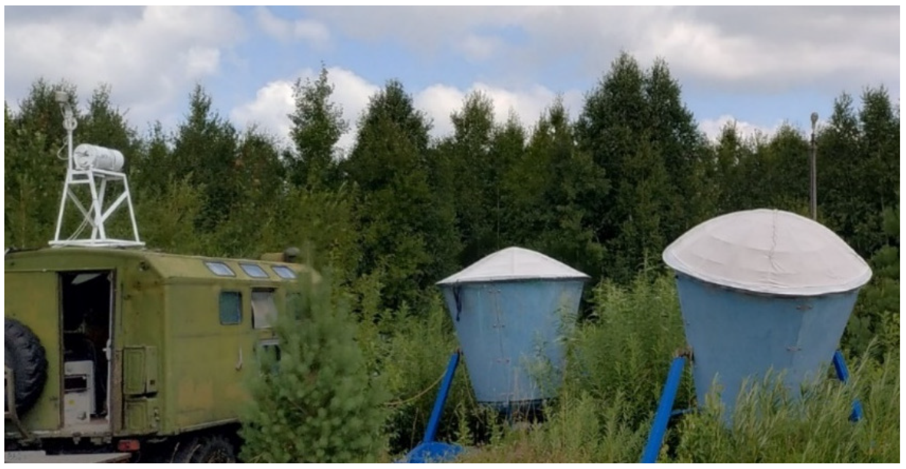
For the analysis, we used the results of measurement by ground-based remote sounding the atmosphere by the temperature and wind profiling complex, consisting of the meteorological temperature profiler MTP-5 (MWR) [22] and the acoustic meteorological locator Volna-4M (sodar) [27]. The complex was located on the territory of the Basic Experimental Complex of the V.E. Zuev Institute of Atmospheric Optics, Siberian Branch, Russian Academy of Sciences (IOA SB RAS), located in the suburbs of Tomsk (an open meadow surrounded by forest plantations up to 10–15 m high) with coordinates 56°28′54″ N, 85°06′00″ E (Figure 1).

Figure 1.
Photo of the meteorological temperature profiler MTP-5 (left) and the acoustic meteorological locator “Volna-4M” (sodar, (right)) on the territory of the Basic Experimental Complex IOA SB RAS, 2020.
The MTP-5 is a self-calibrating, self-testing single-channel scanning microwave meteorological temperature profiler [22]. MTP-5 has been used for measuring temperature profiles from the level of installation to the height of 1000 m in all weather conditions. The instrument passed the series of international comparisons with different alternative measurement systems: radiosondes, RASS, meteorological masts, etc. [31]. Following the results of the series of comparisons and tests in 2011, the instrument is included in the “Quality Assurance Guidance for the Collection of Meteorological Data Using Passive Radiometers” worked out by the U.S. Environmental Protection Agency [32]. The tropospheric temperature profile T(H) is found from the angular spectrum of the atmospheric brightness temperature in the absorption band of molecular oxygen O2 near the frequency ν ≈ 60 GHz by solving the inverse problem. The connection between the measured angular spectrum of the brightness temperature TB(θ) and the temperature profile T(H) is determined by the Fredholm nonlinear integral equation of the first kind. Upon linearization and algebraization (i.e., after passing from integration to summation), the equation is solved by the statistical regularization method. Thermal sounding of the troposphere is carried out at the frequency ν = 56.6 GHz for eight zenith angles in the range θ = 0°–86°. The effective height of the thermal sounding is about 1.3 km. Approximately 80% of the atmospheric radiation is formed in this layer. Effective retrieval of the tropospheric temperature profile T(H) is also performed in the altitude range h = 0–1.3 km. The rms deviation (RMSD) of the T(H) profile in the range of effective sounding heights h = 0–1.3 km is 0.3–1.2 °C, accordingly [22]. We verified the reliability of measuring temperature profiles using the MTP-5 instrument by comparing them with radiosonde measurements [33]. A sufficient accuracy with a single-channel microwave radiometer (MTP-5) in the lower layers of the PBL allows to get a representative description of the dynamics of characteristics up to 1 km.
Meteorological acoustic locator (sodar) is a device capable of diagnosing the microstructure of the turbulent component of the temperature field. Sodar signals are proportional to the dispersion of air temperature in the atmospheric layer of the volume V at a certain height H.
The higher the altitude, the bigger the value (up to tens of thousands of cubic meters for sodar Volna-4M at altitudes of about 1 km with a sounding pulse duration of 0.15 s at carrier frequencies from 1.9 to 2.3 kHz).
For the data analysis, the results of daily measurements in July and September 2020 were used. The MTP-5 measured temperature profiles in the range of heights from the installation level (4 m from the surface, see Figure 1) to an altitude of 1 km with a time step of 5 min and a height step of 50 m.
Sodar provided measurements in the range of 45 to 1000 m with a time step of about 10 s. As a result, the simultaneous operation of MTP-5 and sodar amounted to 509 h (68%) in July and 599 h (83%) in September 2020. For the data analysis, the synchronized and averaged 10 min values are used as source.
At the observation point (56°28′53″ N, 85°06′00″ E), the local time of sunrise varied from 04:32 to 05:20 in July and from 06:24 to 07:21 in September, and the time of sunset is from 22:13 to 21:32 in July and from 20:15 to 18:58 in September.
3. Temperature Regime of the Experiment Period
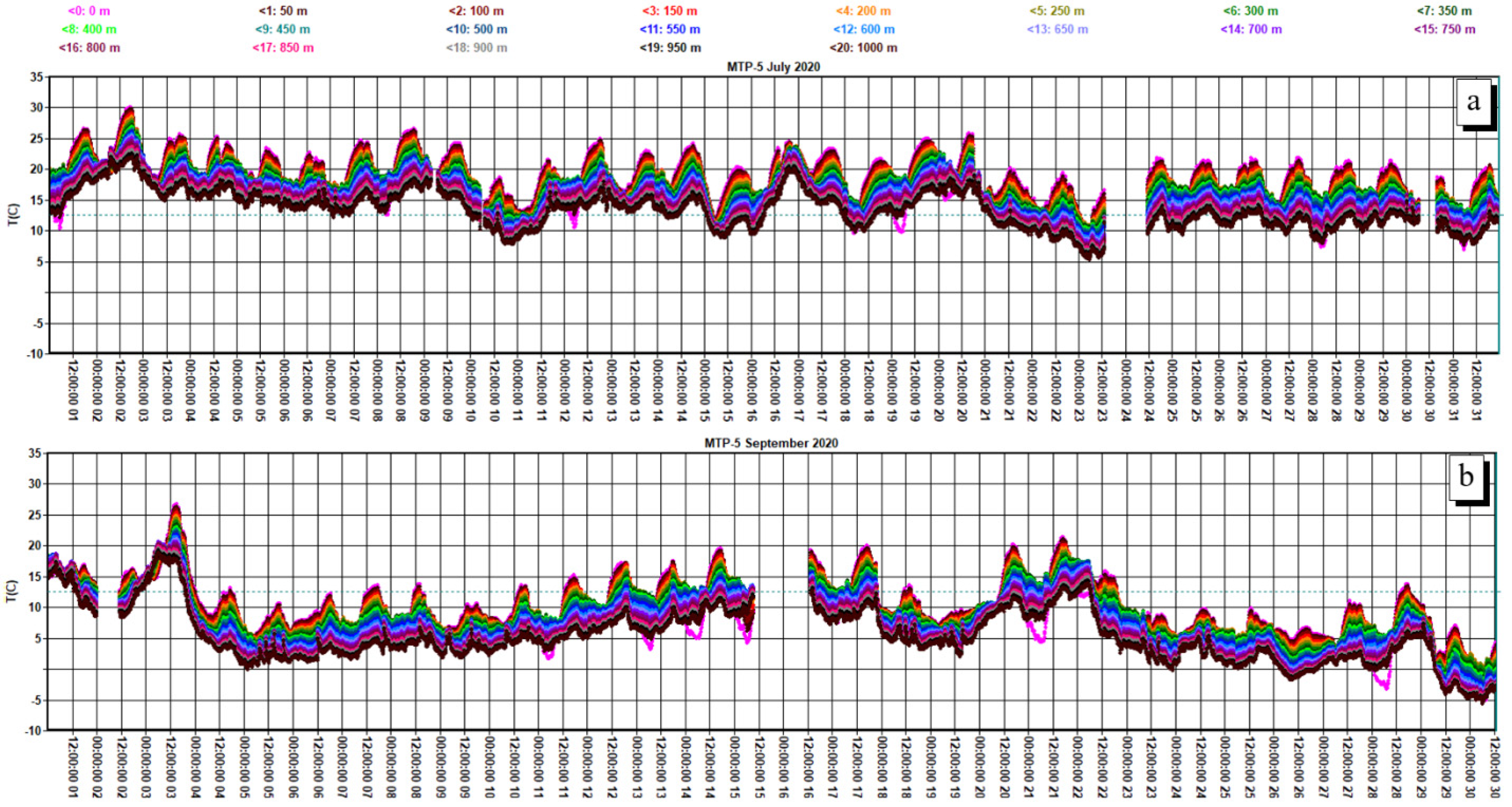
The air temperature profile time series (MTP-5 data) in the 0–1 km layer in July and September 2020 is shown in Figure 2. Note that the influence of clouds and precipitations was not considered in the analysis.

Figure 2.
MTP-5 temperature profiles time series (each color for each height with step 50 m) in the 0–1 km layer in July (a) and September (b) 2020.
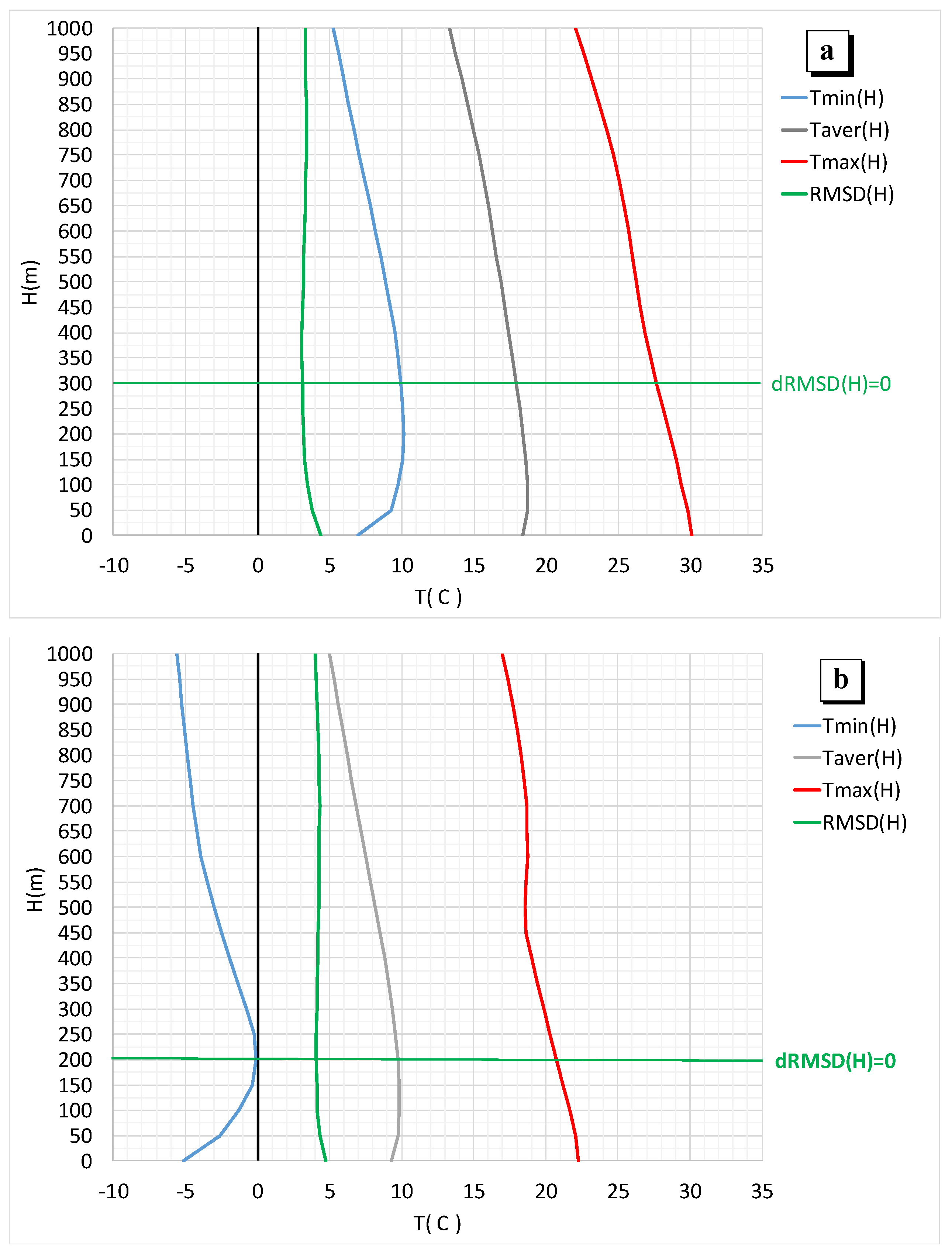
Figure 3 and Table 1 show the statistical distribution of the temperature profiles values in heights from 0 to 1000 m as profile of the minimums in temperature (Tmin(H)), profile of the averages values (Taver(H)), profile of the maximum values (Tmax(H)) and the profile of rms deviation (RMSD(H)) for all month data of July and September.
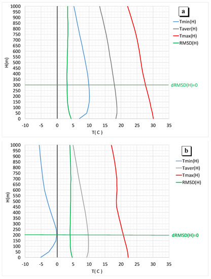
Figure 3.
Statistical parameters of temperature profiles values in the 0–1 km PBL altitude range for July (a) and September (b) 2020 by MTP-5 data.

Table 1.
Statistical distribution of the temperature profiles values.
The variability of the temperatures values for July was mainly concentrated at heights below 300 m (the level above which increment dRMSD = 0, green line on Figure 3). For September, variability was observed in the whole 0–1 km layer and it is difficult to dedicate a level when the increment of the dRMSD = 0. In absolute values, it is 200 m, but not as prominent as in July.
4. PBL Parameters by Sodar Data
Sodar registers backscattered acoustic sounding signals from air layers (precisely, from a layer, the dimensions of which are related to the duration of the sounding pulse and the width of the sodar antenna pattern), the values of which are proportional to the dispersion of the air temperature at a given height. According to our estimates (see the works in [34,35]), the used sodar receives signals from those layers in which the structural characteristic of air temperature has values > 10−5 at (K2/m2/3) at moderate levels of ambient noise. If [36], where is the air temperature dispersion and is the outer scale of temperature turbulence, focus on in the surface layer at the observation point ( ~ 8 ÷ 10 m, see in [37]), then in the controlled area PBL it was possible to determine dispersion estimates > 10−5 (K2). Therefore, sodar can provide sufficient sensitivity to determine the height of the layer of intense turbulent heat exchange (Hm). However, at those noise levels (external and instrumental) that were during the observation periods, we can suppose that sodar provided reliable data only at > 10−4 (K2). In this regard, it can be assumed that there was some underestimation of the height of the level with an increased dispersion of air temperature, especially during daytime.
Visualization of sodar signals is usually done in the form of “echograms”—the height-temporal distribution of their amplitude. The height Hm was determined from the echograms and corresponded to the height at which the “useful” sodar signals became comparable to the level of the surrounding noise. It was assumed that intense turbulent heat transfer starts from the surface and does not have any “breaks” up to the height Hm.
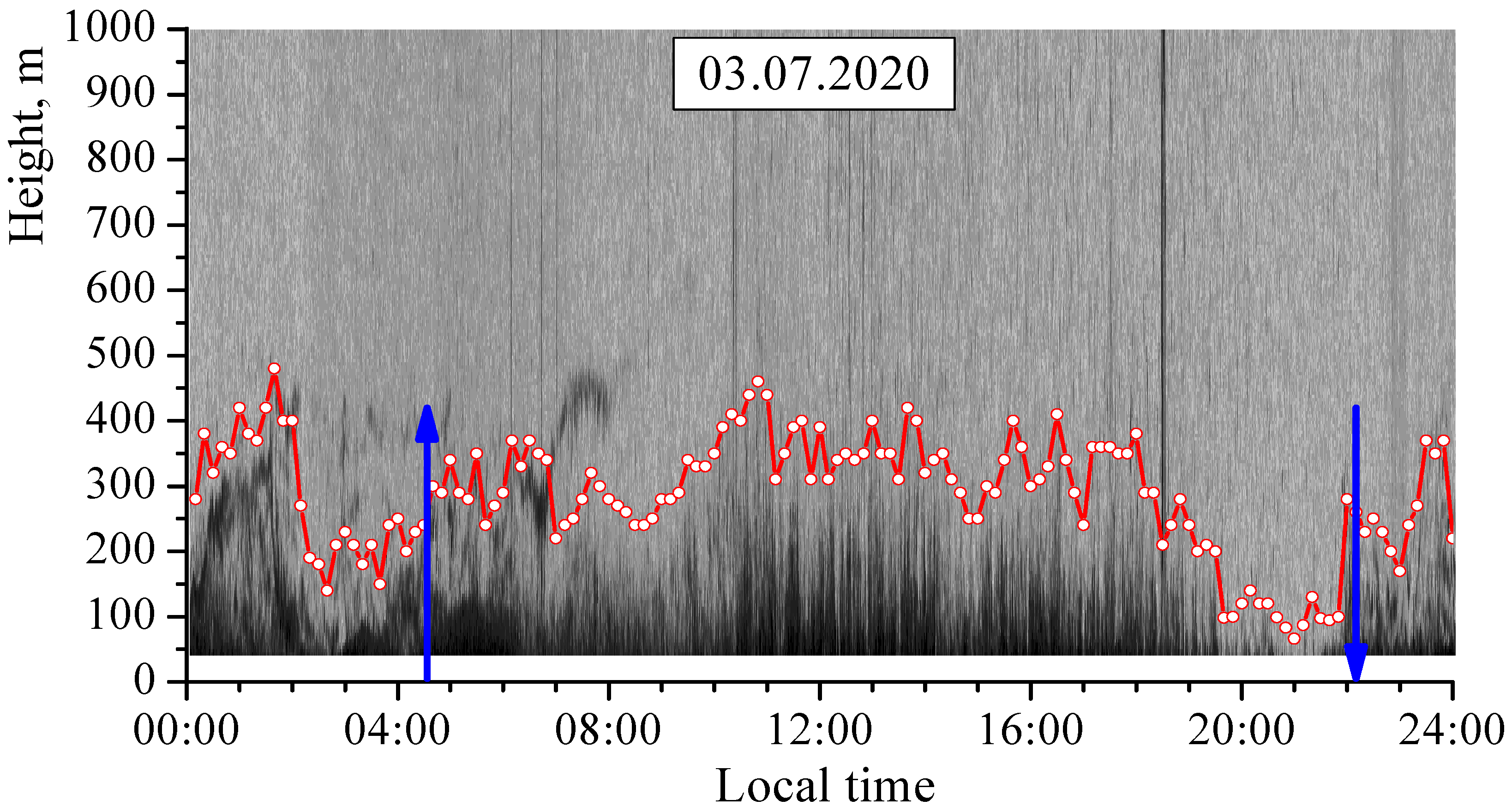
Figure 4 shows the example of an original echogram, on which the heights (dotted line) are plotted, obtained as average values over a time interval of Δt = 10 min. The example demonstrates the presence of separate layers with increased temperature dispersion, located above and not connected by turbulent heat exchange with the surface layer (see period 02: 00–08: 00). According to our estimates, the errors of determination can be up to 30–50 m, and in conditions of high levels of ambient noise, it is somewhat higher. Nevertheless, we believe that the results with calculations Hm presented provide an adequate idea of the range of variation of these heights in the range of 0 to 1 km of the PBL.
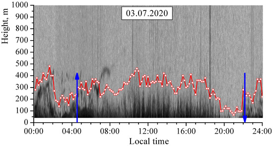
Figure 4.
The original sodar echogram with the plotted height Hm graph (red line with dots). Times of sunrise and sunset were 04:36 and 22:11, respectively (indicated by blue arrows).
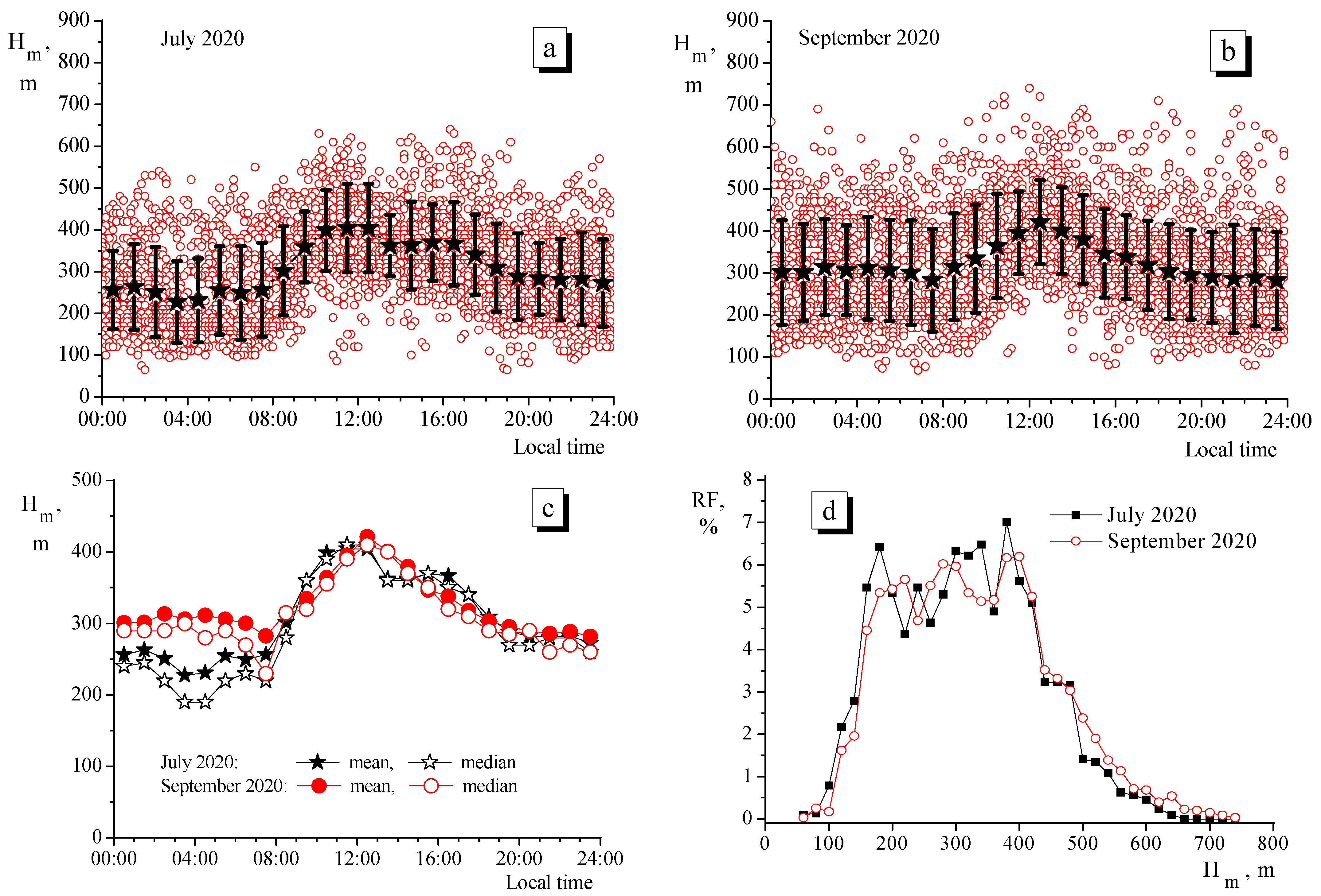
In Figure 5, the daily variation and some statistical characteristics of the Hm in the compared measurement periods are shown. Comparing the diagrams of the average daily variation in July and September (Figure 5c), we can conclude that, overall, they are similar, but in September in the period 00:00–07:00, the turbulent heat transfer spreads slightly higher than in July. This effect is due to the fact that in September the wind speed during the indicated period of the day was generally somewhat higher than in July, and intensified the processes of turbulent heat transfer, expanding the region with increased temperature dispersion (even with temperature inversions in the PBL).
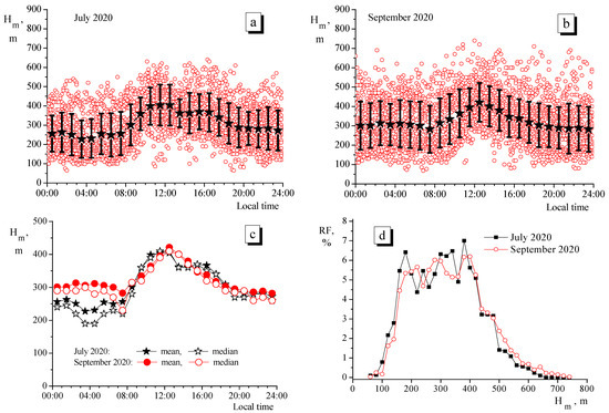
Figure 5.
The daily variation of the height Hm in July (a) and in September (b) 2020, indicating the average values (black asterisks) and its RMSD (black segments); (c) daily variation of mean and median values; (d) relative frequency of the Hm.
It is useful to analyze the statistical characteristic RF, which is the relative frequency. It allows to roughly estimate the repeatability of values in a range of Hm heights. In Figure 5d, RF (as a percentage of total cases) are shown for July and September.
The wind speed in the surface layer during the periods under consideration varied from values close to zero up to 6–7 m/s (estimates for 10-min time intervals at an altitude of 10 m). During the daytime, the wind speed was usually higher than at night. Moreover, in September, the wind speed varied more significantly during the day than in July.
5. PBL Characteristics from Temperature Stratification Data
To analyze the dependence and for comparisons of the temperature regime parameters in the heights range of 0 to 1 km, PBL parameters have been calculated from the acoustic and microwave remote sensing data.
For days with good weather, the PBL has a well-defined structure and diurnal cycle [1,38], which leads to the development of a convective boundary layer (CBL), also called a mixing layer, during the day and a stable boundary layer (SBL) at night [1]. The SBL can be characterized by surface-based temperature inversion (SBI), i.e., inversion with a base height starting at the surface (Hbase = 0) [1,38]. In the investigation, we used a classification adapted to the conditions of our observations (see Table 2) [1].
Table 2.
List of abbreviations.
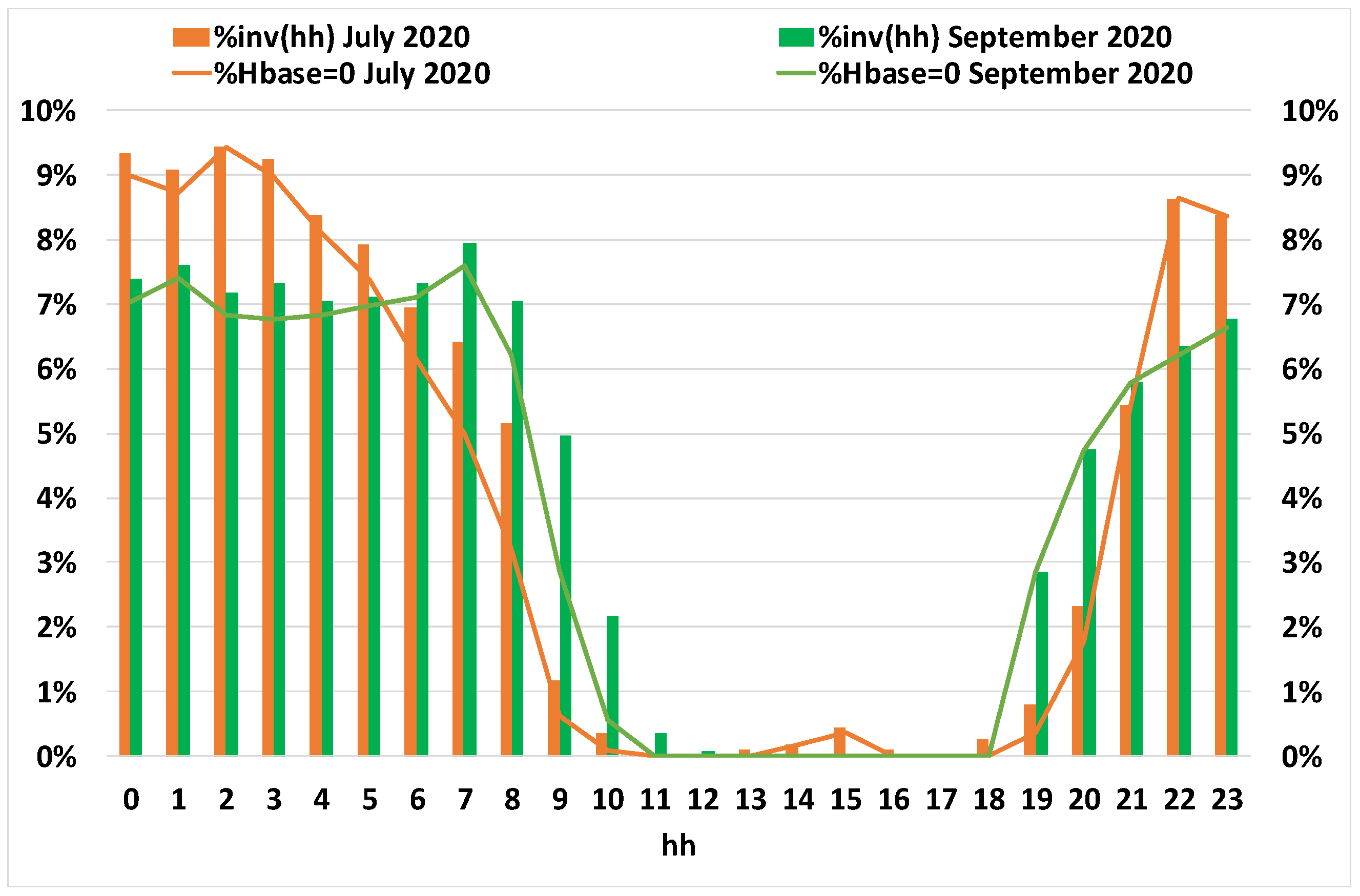
Figure 6 shows that in most cases the top height of the temperature inversion (Htop) is equivalent to the thickness of the inversion layer, because the inversions started from surface Hbase = 0 (almost all inversions are during nighttime and surface-based ones).

Figure 6.
Distribution of the temperature inversions by time of day (hh) and the number of surface based inversions (Hbase = 0) in July and September 2020.
In calculations of the mixing layer height HPC, we used the Parcel method [1,4,10,15] with the refinement introduced by Kuznetsova et al. [21] and methodically approved by Roshydromet in 2010. With this modification, the HPC height is dedicated by the intersection of the measured T(H) profile and the “dry” adiabatic profile has been shifted by 0.5 °C: TK(H) ≈ T(H = 0) − 0.0098 × H + 0.5.
Considering the periods of sunrise–sunset and the dependence of the PBL characteristics according to the data on the dynamics of T(H), we have determined the time ranges for SBL and CBL periods. Table 3 shows the intervals in hours for the SBL and CBL periods and transitions. Different periods are characterized by a different set of parameters for analysis. For night-time (SBL), we compared Hm with temperature inversion (SBI) characteristics, and for daytime (CBL), comparisons were made with Hm and HPC height.
Table 3.
The intervals in hours for the SBL and CBL periods and transitions.
6. SBL Characteristics
For the SBL period, Hm has been compared with the top of the temperature inversion (Htop), with the strength of the temperature inversion (ΔTi) and with the thickness of the temperature inversion layer (ΔHi). During the observation period, there was a sufficient number of cases of temperature inversions of 25 and 29% of the total measurement period. The characteristics of the total number of profiles and the number of cases with temperature inversion are presented in Table 4.
Table 4.
The characteristics of the total number of profiles and the number of cases with temperature inversion.
We carried out a sufficiently detailed analysis of the temperature inversion cases to study the special behavior of turbulent heat exchange in the range of 0 to 1 km of PBL. We investigated the dependencies when this heat exchange covered the entire inversion layer, and not only during the period of its final destruction in the morning hours.
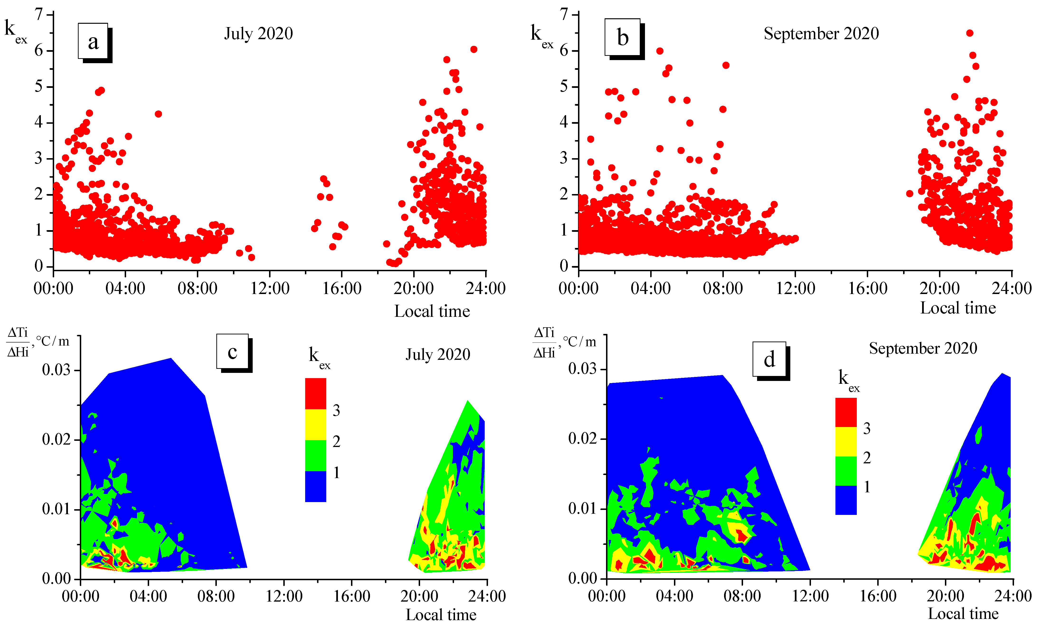
To identify cases of overlap, we use the relation kex = Hm/Htop (overlap index). An overlap takes place if kex > 1, Figure 7a,b shows diagrams of the daily variation of the kex coefficient. According to these plots, the overlapping of the temperature inversion by turbulent heat exchange can take place practically at all intervals of the inversion existence. Estimates show that the option kex > 1 was implemented approximately 40% of this time. Moreover, this was especially active in the evening, when the formation of night temperature inversions began.

Figure 7.
Diurnal variation of the kex overlap index (a) in July and (b) in September 2020; dependence of the overlap index on the time of day and the intensity of the inversion (c) in July and (d) in September 2020.
Obviously, the strength of inversion by temperature ΔTi = T(Htop) − T(Hbase), as well as the inversion layer thickness ΔHi = Htop − Hbase, play a significant role in the overlapping of the inversion by the turbulent heat exchange.
The kex coefficient should depend on the value ΔTi/ΔHi (°C/m) (intensity of the inversion). This dependence within the daily cycle is shown in Figure 7c,d. In the graph in Figure 7c, estimates of kex in the period 10:00 ÷ 19:00 have been excluded due to too small amount of data with temperature inversions. As noted above, the difference in heights ΔHi is shown in most of the cases in Figure 7c,d, corresponding to surface-based temperature inversions, except (in total) 16 h in July and 12 h in September, when elevated temperature inversions were measured.
Therefore, it follows that the temperature inversion in the PBL layer 0–1 km can exist when it is completely covered by turbulent heat exchange if the normalized intensity of the inversion ΔTi/ΔHi (°C/m) is less (very approximately) 0.015 °C/m. Additional conditions for cases with Hm > Htop (kex > 1) require an additional analysis. The effect of overlapping temperature inversions in the 0-1 km PBL layer by turbulent heat exchange is characteristic not only for the warm season, which is represent in this work, but also in winter with long-term implementation of stable stratification. This has been demonstrated in our publications [27,28].
7. SBI Characteristics
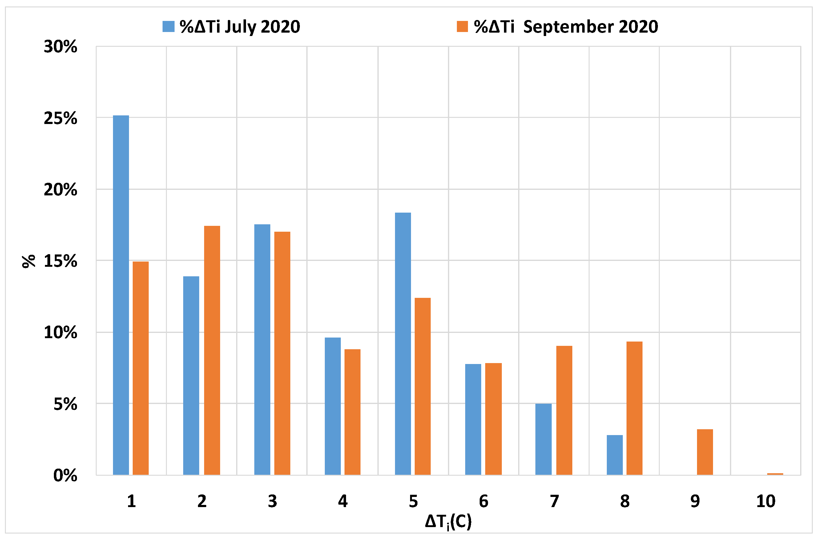
In analyzing the SBI periods, the difference between Hm and Htop was investigated in dependence of the inversion power ΔTi and by the layer thickness ΔHi. When the temperature inversion is surface-based then Hbase = 0 and the top height of the inversion Htop is equivalent to the thickness of the inversion layer ΔHi. Figure 8 and Figure 9 show the statistical distribution of the inversions power ΔTi and for inversion layer thickness ΔHi for both months. Both periods are similar in the distribution of the analyzed values with minor differences. The graphs illustrate the presence of powerful inversions (ΔTi = 3–8 °C) corresponding with a layer thickness ΔHi of 150–300 m. The range of 3 to 8 °C is characterized by the fact that with inversions of such a power in temperature, the difference between Hm and Htop is more often negative for both months (Figure 10).

Figure 8.
Distribution of the temperature inversion power ΔTi in July and September 2020.
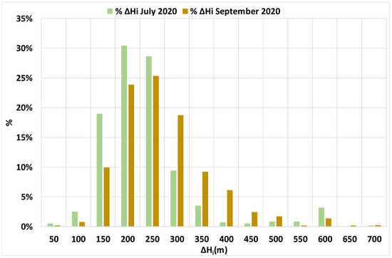
Figure 9.
Distribution of the temperature inversion layer thickness ΔHi in July and September 2020.
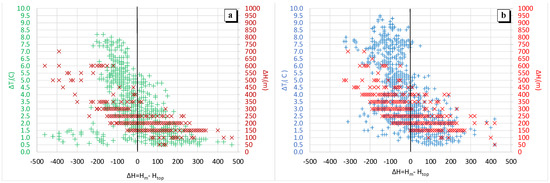
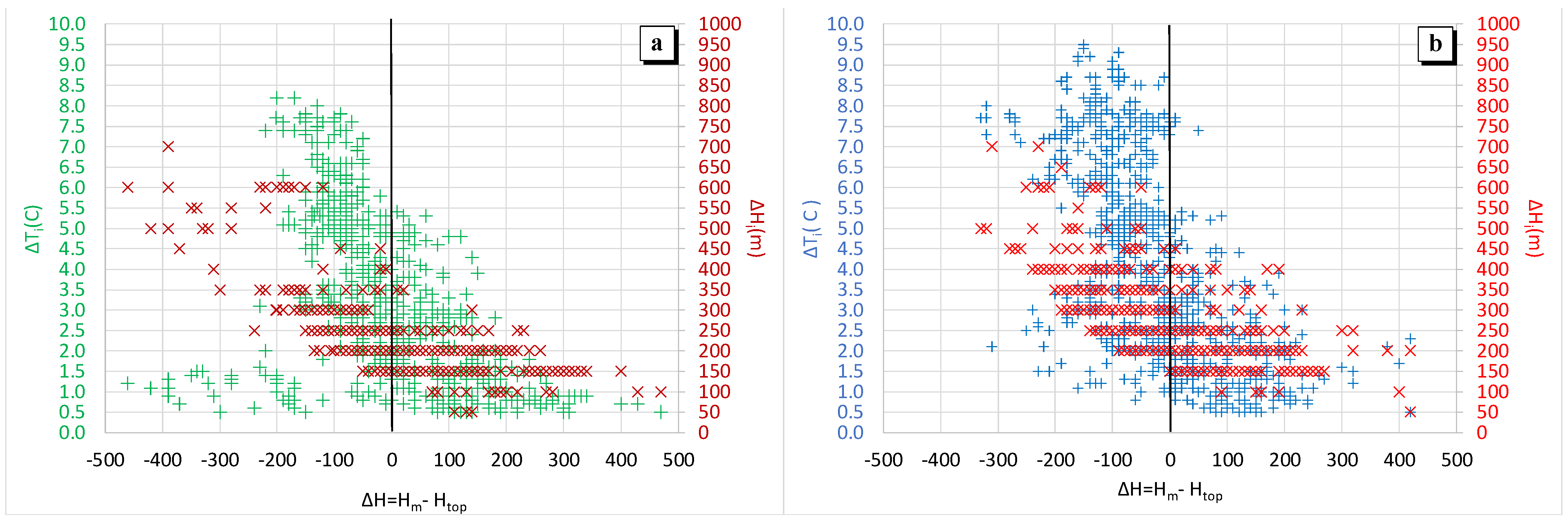
Figure 10.
Graphs of the ΔH = Hm − Htop in dependence of ΔTi and ΔHi: (a) July and (b) September 2020.
To analyze the relations between Hm and Htop, the graphs of the ΔH = Hm − Htop were plotted in dependence on ΔTi (Figure 10, green and blue in left axis) and ΔHi (Figure 10, red in right axis). If ΔH is in range ±50 m, then in 92% of the cases is ΔTi in the range of 1 to 6 °C with a ΔHi ranging from 150 to 250 m in July. For September, 85% of the cases were situations with ΔH = ±50 m, 1 < ΔTi < 6 °C and 150 < ΔHi < 450 m.
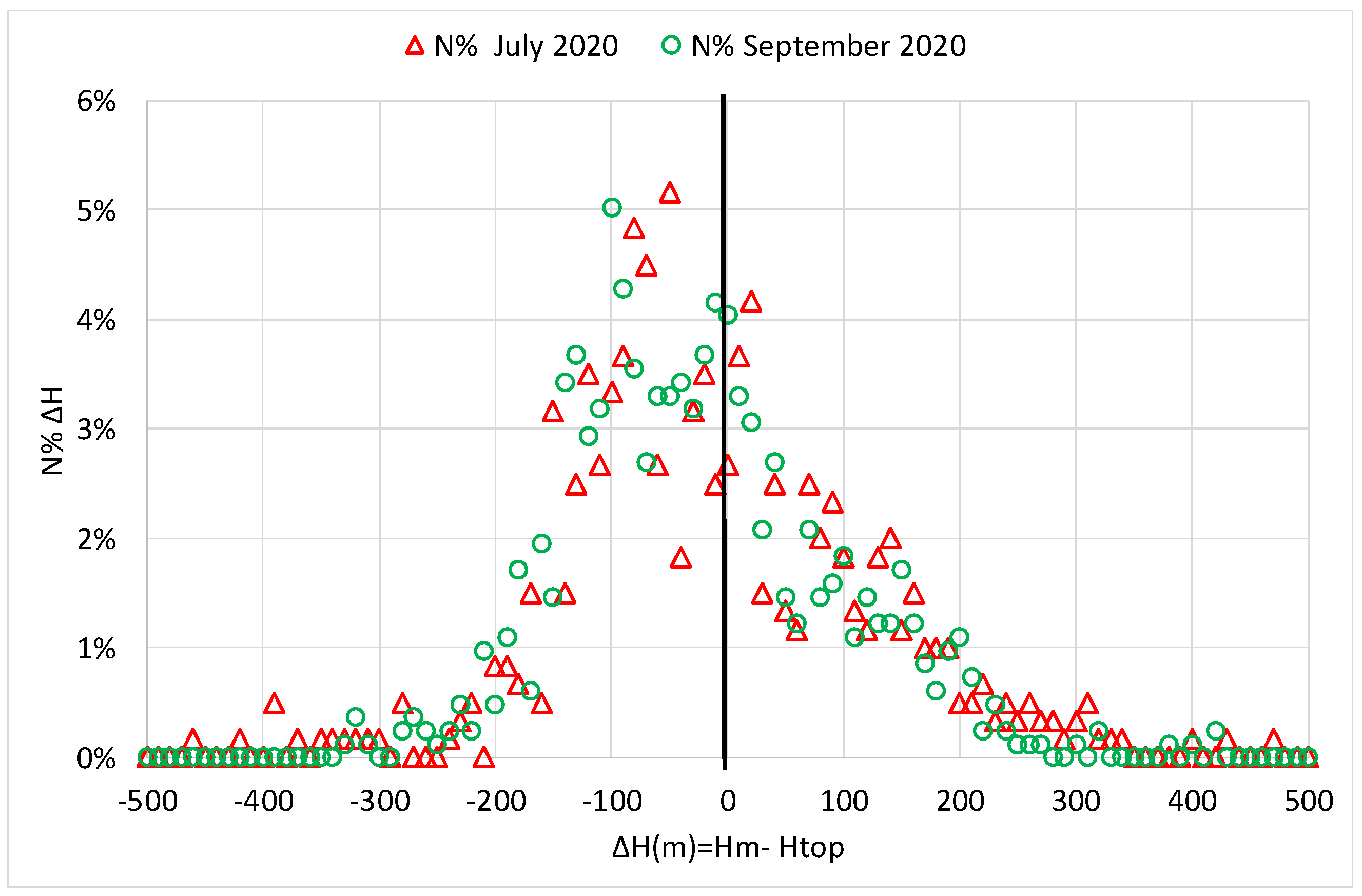
Figure 11 illustrates how the difference ΔH is distributed over the number of cases. ΔH values in the range from −100 to 0 m (Hm < Htop) are more common for both July and September 2020. Table 5 shows that in most cases ΔH < 0 (Hm < Htop). However, the number of cases when ΔH ≥ 0 (Hm ≥ Htop) is significant and is 44% in July and 39% in September 2020.
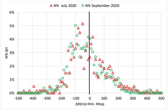
Figure 11.
Distribution of ΔH = Hm − Htop in dependence of the frequency of cases in July (triangles) and in September (dots) 2020.
Table 5.
Distribution of the ΔH (positive and negative) in July and September 2020.
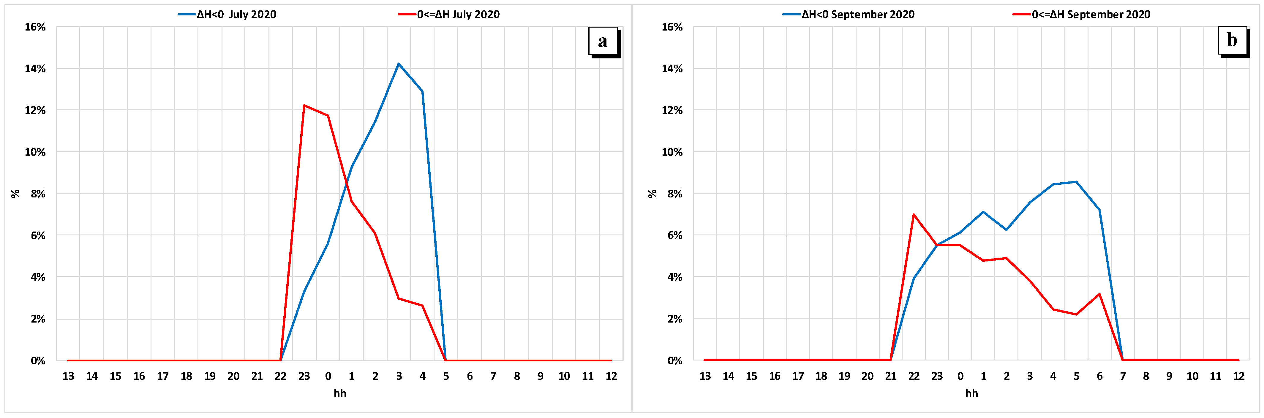
Figure 10, Figure 11 and Figure 12 illustrate the change in the ratio between Hm and Htop in the daily (Figure 12) evolution of PBL in the altitude range of 0 to 1 km. In the transition from CBL to SBL after sunset, the inversions do not yet gain maximum power in terms of temperature ΔTi and layer thickness ΔHi, and the case Hm > Htop (ΔH ≥ 0) occurs most often (Figure 12). According to Figure 10, positive values of ΔH occur mainly at values ΔTi < 4 °C and ΔHi < 300 m.
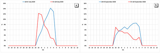
Figure 12.
ΔH = Hm − Htop in the daily PBL cycle for (a) July and (b) September 2020. ΔH ≥ 0—red line, ΔH < 0—blue line.
Close to sunrise, before the transition from SBL to CBL, the inversions are maximum in terms of the temperature difference (ΔTi > 4 °C), the thickness of the inversion layer (ΔHi > 300 m), and Hm < Htop (ΔH < 0) takes place. Thus, the change in the sign of the difference ΔH between Hm and Htop occurred during the night-time cooling of PBL. Note that in September 2020, the change in the sign of ΔH is less pronounced in time of day compared to July (Figure 12b).
8. Mixing Layer Height Characteristics in the Case of CBL
Figure 13 shows the diurnal dynamics of Hm and HPC on the background of the potential temperature gradient field for 3 July 2020. The potential temperature gradient at a height Hj is calculated as γΘ(Hj) = [Θ(Hj) − Θ(Hj−1)]/Δz, where Δz = Hj − Hj−1 = 50 m and Θ(Hj) ≈ T(Hj) + 0.0098 × Hj is the potential temperature profile with a step of 50 m).
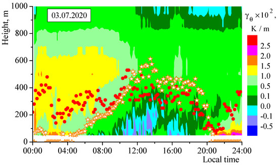
Figure 13.
Diagram of the height-time distribution of the potential temperature gradient (the scale of values is shown to the right of the graph), HPC—asterisks, Hm—red dots.
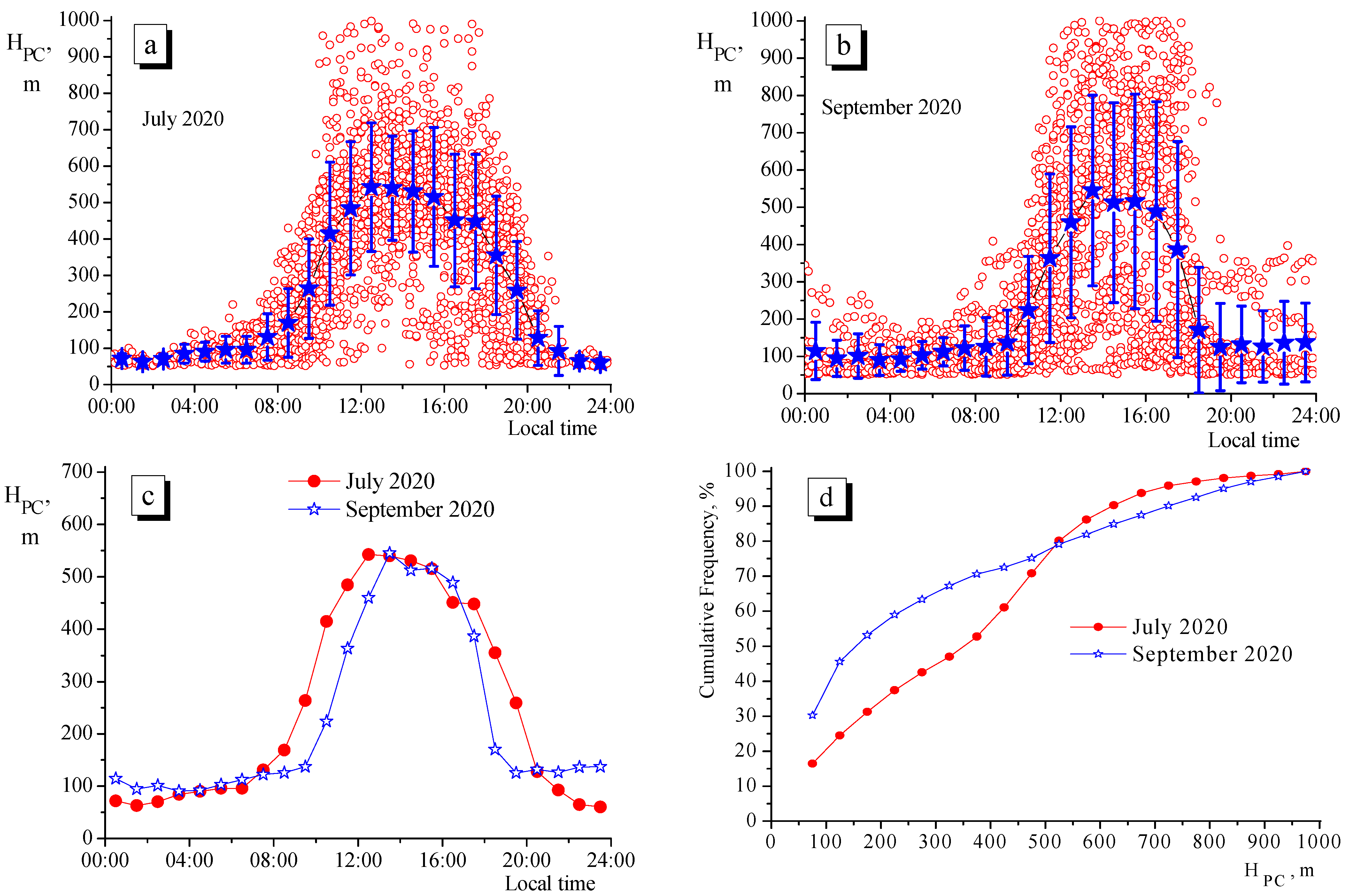
The values HPC were calculated for cases when for the low level of the PBL the condition T(H) − TK(H) < 0 was satisfied, where TK(H) is the “dry” adiabatic profile shifted by 0.5 °C. If the specified inequality took place up to an altitude of 1000 m, then the estimate was marked as 1001 m. Such conditions significantly reduce number of profiles available for calculation HPC, for night-time especially. Calculation of the HPC was applied to the measured profiles to detect daytime PBL parameters in the period of the CBL. This is demonstrated in Figure 14 with a daily evolution of HPC (dots) in July (392 h) and in September (377 h). The figure does not include values of HPC less than 50 m and more than 1000 m; these cases were not included in the calculations. Note, the elevation level of 1000 m was present for 14 h in July and 7 h in September. The hourly averaged values HPC are shown in Figure 14. A comparison of the averaged, hourly values HPC in July and September is shown in Figure 14c, and the cumulative frequency is shown in Figure 14d. According to Figure 14a,b the processes of formation of the mixing layer height values are more diverse in September than in July. Although the ranges of changes in the diurnal variation are approximately the same (considering the difference in the duration of daylight in July and September, Figure 14c.
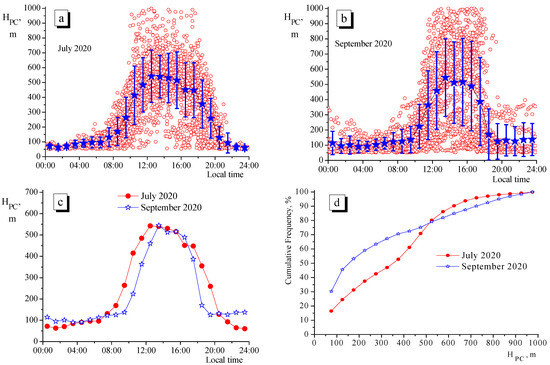
Figure 14.
Diurnal variation (a) in July and (b) in September 2020 showing the mean values (asterisks) and RMSD (segments); (c) comparison of the daily variation of the mean values; and (d) cumulative frequency.
9. Conclusions
Based on the experimental data obtained using the temperature-wind complex (single-channel MWR MTP-5 and acoustic meteorological locator sodar), the height of the mixing layer HPC with height values of the intense turbulent heat exchange Hm have been estimated and compared. The height range from the surface layer up to 1000 m was monitored. The analysis included measurements from July and September 2020. The obtained results for July and for the season changing in September illustrate the repeatability and transformations of PBL characteristics, such as the temperature inversions daily time distributions. For both months, ΔH in dependence of the inversion power by temperature ΔTi and inversions layer thickness ΔHi has been calculated. Note that the character of the ΔH distribution by daily times in September is less pronounced than in July.
According to the results of the analysis, it was found that in 95% of the cases HPC was in the range of 50 < HPC < 700 m in July and 50 < HPC < 850 m in September. The range of Hm (except for ±2.5% of the “edge” values in the distribution of the integral function) was 50 < Hm < 600 m both in July and September. In the daytime, the height HPC was higher than Hm.
For periods with surface-based and elevated air temperature inversions a detailed analysis of the height Hm, i.e., the height of the layer with increased air temperature dispersion characterizing turbulent heat exchange, was carried out. As a result, it was found that at sufficiently long-time intervals (up to 40% of the total time of the existence of inversions) this layer can completely “cover” the inversion without leading to its destruction.
The material presented in this article will be useful for refining the methods and algorithms for modeling the state of the atmospheric boundary layer under temperature inversion conditions. As far as we know, current methods do not take into account the possible effects of overlapping of inversions by turbulent heat transfer. In the future, we plan to carry out a comparative analysis of experimental estimates of the layer height of intense turbulent heat transfer with the stable stratification of the PBL with the models published in the literature for the mixing layer height under such conditions.
Author Contributions
Conceptualization, S.O. and E.M.; methodology, S.O., A.K. and E.M.; software, I.N.; validation, M.S.; formal analysis, I.N.; investigation, S.O., E.M. and A.T.; writing—original draft preparation, S.O., E.M. and M.S.; writing—review and editing, S.O., E.M. and M.S.; supervision, A.K. and A.T. All authors have read and agreed to the published version of the manuscript.
Funding
This research received no external funding.
Conflicts of Interest
The authors declare no conflict of interest.
References
- Coen, M.C.; Praz, C.; Haefele, A.; Ruffieux, D.; Kaufmann, P.; Calpini, B. Determination and climatology of the planetary boundary layer height above the Swiss plateau by in situ and remote sensing measurements as well as by the COSMO-2 model. Atmos. Chem. Phys. 2014, 14, 13205–13221. [Google Scholar] [CrossRef] [Green Version]
- Huang, M.; Gao, Z.; Miao, S.; Chen, F.; LeMone, M.A.; Li, J.; Hu, F.; Wang, L. Estimate of Boundary-Layer Depth Over Beijing, China, Using Doppler Lidar Data During SURF-2015. Bound. Layer Meteorol. 2017, 162, 503–522. [Google Scholar] [CrossRef] [Green Version]
- Li, H.; Yang, Y.; Hu, X.-M.; Huang, Z.; Wang, G.; Zhang, B.; Zhang, T. Evaluation of retrieval methods of daytime convective boundary layer height based on lidar data. J. Geoph. Res. Atmos. 2017, 122, 4578–4593. [Google Scholar] [CrossRef]
- Danchovski, V. Summertime Urban Mixing Layer Height over Sofia, Bulgaria. Atmosphere 2019, 10, 36. [Google Scholar] [CrossRef] [Green Version]
- Sawyer, V.; Li, Z. Detection, variation and intercomparision of the planetary boundary layer depth from radiosonde, lidar and infrared spectrometer. Atmos. Environ. 2013, 79, 518–528. [Google Scholar] [CrossRef]
- Hicks, M.; Demoz, B.; Vermeesch, K.; Atkinson, D. Intercomparision of mixing heights from national weather service celiometer test sites and collocated radiosondes. J. Atmos. Ocean. Technol. 2019, 36, 129–137. [Google Scholar] [CrossRef] [Green Version]
- Lee, J.; Hong, J.-W.; Lee, K.; Hong, J.; Velasco, E.; Lim, Y.J.; Lee, J.B.; Nam, K.; Park, J. Ceilometer Monitoring of Boundary-Layer Height and Its Application in Evaluating the Dilution Effect on Air Pollution. Bound. Layer Meteorol. 2019, 172, 435–455. [Google Scholar] [CrossRef] [Green Version]
- Feudo, T.L.; Calidonna, C.R.; Elenio Avolio, E.; Sempreviva, A.M. Boundary Layer Integrating Surface Measurements and Ground-Based Remote Sensing. Sensors 2020, 20, 6516. [Google Scholar] [CrossRef] [PubMed]
- Zhong, T.; Wang, N.; Shen, X.; Xiao, D.; Xiang, Z.; Liu, D. Determination of Planetary Boundary Layer height with Lidar Signals Using Maximum Limited Height Initialization and Range Restriction (MLHI-RR). Remote Sens. 2020, 12, 2272. [Google Scholar] [CrossRef]
- Matsui, I.; Sugimoto, N.; Maksyutov, S.; Inoue, G.; Kadygrov, E.; Vyazankin, S. Comparison of Atmospheric Boundary Layer Structure Measured with a Microwave Temperature Profiler and Mie Scattering Lidar. Jpn. J. Appl. Phys. 1996, 35, 2168–2169. [Google Scholar] [CrossRef]
- Lee, T.R.; De Wekker, S.F.J. Estimating Daytime Planetary Boundary Layer Heights over a Valley from Rawinsonde Observations at a Nearby Airport: An Application to the Page Valley in Virginia, United States. J. Appl. Meteorol. Climatol. 2016, 55, 791–809. [Google Scholar] [CrossRef]
- Lee, T.R.; Pal, S. The Impact of Height-Independent Errors in State Variables on the Determination of the Daytime Atmospheric Boundary Layer Depth Using the Bulk Richardson Approach. J. Atmos. Ocean. Technol. 2021, 38, 47–61. [Google Scholar] [CrossRef]
- Gu, J.; Zhang, Y.H.; Yang, N.; Wang, R. Diurnal variability of the planetary boundary layer height estimated from radiosonde data. Earth Planet. Phys. 2020, 4, 479–492. [Google Scholar] [CrossRef]
- Dai, C.; Wang, Q.; Kalogiros, J.A.; Lenschow, D.H.; Gao, Z.; Zhou, M. Determining boundary-layer height from aircraft measurements. Bound. Layer Meteorol. 2014, 152, 277–302. [Google Scholar] [CrossRef]
- Kotthaus, S.; Haeffelin, M.; Drouin, M.-A.; Dupont, J.-C.; Grimmond, S.; Haefele, A.; Hervo, M.; Poltera, Y.; Wiegner, M. Tailored Algorithms for the Detection of the Atmospheric Boundary Layer Height from Common Automatic Lidars and Ceilometers (ALC). Remote Sens. 2020, 12, 3259. [Google Scholar] [CrossRef]
- Hemingway, B.L.; Frazier, A.E.; Elbing, B.R.; Jacob, J.D. High-resolution estimation and spatial interpolation of temperature structure in the atmospheric boundary layer using a small unmanned aircraft system. Bound. Layer Meteorol. 2020, 175, 397–416. [Google Scholar] [CrossRef]
- Baserud, L.; Reuder, J.; Jonassen, M.O.; Bonin, T.A.; Chilson, P.B.; Jiménez, M.A.; Durand, P. Potential and limitations in estimating sensible-heat-flux profiles from consecutive temperature profiles using remotely-piloted aircraft systems. Bound. Layer Meteorol. 2020, 174, 145–177. [Google Scholar] [CrossRef] [Green Version]
- Tjernström, M.; Mauritsen, T. Mesoscale Variability in the Summer Arctic Boundary Layer. Bound. Layer Meteorol. 2009, 130, 383–406. [Google Scholar] [CrossRef]
- Wang, Z.; Cao, X.; Zhang, L.; Notholt, J.; Zhou, B.; Liu, R.; Zhang, B. Lidar measurement of planetary boundary layer height and comparison with microwave profiling radiometer observation. Atmos. Meas. Tech. 2012, 5, 1965–1972. [Google Scholar] [CrossRef] [Green Version]
- Friedrich, K.; Lundquist, J.K.; Aitken, M.; Kalina, E.A.; Marshall, R.F. Stability and turbulence in the atmospheric boundary layer: A comparison of remote sensing and tower observations. Geophys. Res. Lett. 2012, 39, L03801. [Google Scholar] [CrossRef] [Green Version]
- Methodical Office of the Hydrometeorological Center of Russia. Available online: http://method.meteorf.ru/norma/rec/profile.pdf (accessed on 25 September 2021).
- Ilyin, G.N.; Troitsky, A.V. Determining the Tropospheric Delay of a Radio Signal by the Radiometric Method. Radiophys. Quantum Electron. 2017, 60, 291–299. [Google Scholar] [CrossRef]
- Casasanta, G.; Pietroni, I.; Petenko, I.; Argentini, S. Observed and modelled convective mixing-layer height at Dome C, Antarctica. Bound. Layer Meteorol. 2014, 151, 597–609. [Google Scholar] [CrossRef] [Green Version]
- Petenko, I.; Argentini, S.; Casasanta, G.; Genthon, C.; Kallistratova, M. Stable surface-based turbulent layer during the polar winter at Dome C, Antarctica: Sodar and in situ observations. Bound. Layer Meteorol. 2019, 171, 101–128. [Google Scholar] [CrossRef]
- Van der Linden, S.J.A.; Edwards, J.M.; Van Heerwaarden, C.h.C.; Vignon, E.; Genthon, C.; Petenko, I.; Baas, P.; Jonker, H.J.J.; Van de Wiel, B.J.H. Large-eddy simulations of the steady wintertime Antarctic boundary layer. Bound. Layer Meteorol. 2019, 173, 165–192. [Google Scholar] [CrossRef] [Green Version]
- Lokoshchenko, M.A. Long-Term Sodar Observations in Moscow and a New Approach to Potential Mixing Determination by Radiosonde Data. J. Atmos. Ocean. Technol. 2002, 19, 1151–1162. [Google Scholar] [CrossRef]
- Odintsov, S.L.; Gladkikh, V.A.; Kamardin, A.P.; Nevzorova, I.V. Height of the Region of Intense Turbulent Heat Exchange in a Stably Stratified Atmospheric Boundary Layer: Part 1–Evaluation Technique and Statistics. Atmos. Ocean. Opt. 2021, 34, 34–44. [Google Scholar] [CrossRef]
- Odintsov, S.L.; Gladkikh, V.A.; Kamardin, A.P.; Nevzorova, I.V. Height of the Region of Intense Turbulent Heat Exchange in a Stably Stratified Boundary Layer of the Atmosphere. Part 2: Relationship with Surface Meteorological Parameters. Atmos. Ocean. Opt. 2021, 34, 117–127. [Google Scholar] [CrossRef]
- Emeis, S.; Schäfer, K.; Münkel, C. Surface-based remote sensing of the mixing-layer height—A review. Meteorol. Z. 2008, 17, 621–630. [Google Scholar] [CrossRef]
- Zhang, H.; Zhang, X.; Li, Q.; Cai, X.; Fan, S.; Song, Y.; Hu, F.; Che, H.; Quan, J.; Kang, L.; et al. Research Progress on Estimation of the Atmospheric Boundary Layer Height. J. Meteorol. Res. 2020, 34, 482–498. [Google Scholar] [CrossRef]
- Koldaev, A.; Miller, E.; Troitsky, A.; Sarichev, S. Experimental Study of Rain-induced Accuracy Limits for Microwave Remote Temperature Profiling. In Proceedings of the WMO Technical Conference on Meteorological and Environmental Instruments and Methods of Observation, Helsinki, Finland, 30 August–1 September 2010. [Google Scholar]
- United States Environmental Protection Agency. Available online: https://nepis.epa.gov/Exe/ZyPDF.cgi/P100FC49.PDF?Dockey=P100FC49.PDF (accessed on 25 September 2021).
- Odintsov, S.L.; Gladkikh, V.A.; Kamardin, A.P.; Mamyshev, V.P.; Nevzorova, I.V. Estimates of the Refractive Index and Regular Refraction of Optical Waves in the Atmospheric Boundary Layer: Part 1, Refractive Index. Atmos. Ocean. Opt. 2018, 31, 437–444. [Google Scholar] [CrossRef]
- Kamardin, A.P.; Odintsov, S.L. Height Profiles of the Structure Characteristic of Air Temperature in the Atmospheric Boundary Layer from Sodar Measurements. Atmos. Ocean. Opt. 2017, 30, 33–38. [Google Scholar] [CrossRef]
- Odintsov, S.L.; Gladkikh, V.A.; Kamardin, A.P.; Mamyshev, V.P.; Nevzorova, I.V. Results of Acoustic Diagnostics of Atmospheric Boundary Layer in Estimation of the Turbulence Effect on Laser Beam Parameters. Atmos. Ocean. Opt. 2018, 31, 553–563. [Google Scholar] [CrossRef]
- Tatarskii, V.I. The Effects of the Turbulent Atmosphere on Wave Propagation, translated from Russian. Isr. Program Sci. Transl. Jerus. 1971, 1971, 471. [Google Scholar]
- Gladkikh, V.A.; Nevzorova, I.V.; Odintsov, S.L. Statistics of Outer Turbulence Scales in the Surface Air Layer. Atmos. Ocean. Opt. 2019, 32, 450–458. [Google Scholar] [CrossRef]
- Stull, R.B. An Introduction to Boundary Layer Meteorology; Kluwer Academic Publishers: Dordrecht, The Netherlands; Boston, MA, USA; London, UK, 1988; Volume 13. [Google Scholar]
- Holzworth, G.C. Estimates of mean maximum mixing depths in the contiguous united states. Mon. Weather. Rev. 1964, 92, 235–242. [Google Scholar] [CrossRef] [Green Version]
- Fisher, B.E.A.; Erbrink, J.J.; Finardi, S.; Jeannet, P.; Joffre, S.; Morselli, M.G.; Pechinger, U.; Seibert, P.; Thomson, D.J. Cost Action 710-Final Report: Harmonisation of the Pre-Processing of Meteorological Data for Atmospheric Dispersion Models; Office for Official Publications of the European Communities: Belgium, Brussels, 1998. [Google Scholar]


Publisher’s Note: MDPI stays neutral with regard to jurisdictional claims in published maps and institutional affiliations. |
© 2021 by the authors. Licensee MDPI, Basel, Switzerland. This article is an open access article distributed under the terms and conditions of the Creative Commons Attribution (CC BY) license (https://creativecommons.org/licenses/by/4.0/).