Abstract
Convolutional neural networks (CNN) have been used increasingly in several land-use classification tasks, but there is a need to further investigate its potential. This study aims to evaluate the performance of CNN methods for land classification and to identify land-use (LU) change. Eight transferred CNN-based models were fully evaluated on remote sensing data for LU scene classification using three pre-trained CNN models AlexNet, GoogLeNet, and VGGNet. The classification accuracy of all the models ranges from 95% to 98% with the best-performed method the transferred CNN model combined with support vector machine (SVM) as feature classifier (CNN-SVM). The transferred CNN-SVM model was then applied to orthophotos of the northeastern Cloverdale as part of the City of Surrey, Canada from 2004 to 2017 to perform LU classification and LU change analysis. Two sources of datasets were used to train the CNN–SVM model to solve a practical issue with the limited data. The obtained results indicated that residential areas were expanding by creating higher density, while green areas and low-density residential areas were decreasing over the years, which accurately indicates the trend of LU change in the community of Cloverdale study area.
1. Introduction
Land-use (LU) represents the human use of the natural environment for economic, urban, recreational, conservational and governmental purposes. Land-cover (LC) represents how a region of the earth surface is covered by physical features such as vegetation, water, forest or other [1]. In modern history, the worldwide growth of population has brought significant challenges to society and the environment, such as the increasing demand for housings, food, natural resources and basic services [2]. These have resulted in land-use and land-cover (LULC) changes that have caused adverse effects on the natural environments [3]. The need for efficient land-use planning and management is increasing, not only to eliminate the negative effects of historical LU decisions but also to make future communities healthier and more sustainable [4]. Therefore, there is a need for more advanced computational methods to analyze geospatial data from the Earth’s surface to quantify and better understand the complex dynamics of LULC change processes.
Remote sensing (RS) datasets provide significant information documenting the land-use and land-cover processes [5]. RS datasets provide coverages from regional to global scales [6]. Interpretation of RS datasets is a major way to understand the status and changes in both the natural and built environments. In recent decades, RS sensors and techniques have become increasingly sophisticated. They can provide a large volume of datasets with high quality and fine spatial resolution.
Due to easier access to data with higher volume and better quality as well as the development of advanced graphics processing units (GPU), deep learning (DL) has been widely promoted in many recent scientific literature. DL consists of a collection of algorithms as the subset of machine learning (ML), specializing in learning hierarchy of concepts from very big data. DL methods have achieved incredible accuracy especially in classification tasks in areas such as speech recognition, computer vision, video analysis, and natural language processing [7,8]. Some of the well-known deep learning algorithms include convolutional neural networks (CNN) [9,10], recurrent neural networks (RNN) [11], deep belief networks (DBN) [12], and stacked auto-encoders (SAE) [13]. This study will apply the CNN algorithm to LU analysis.
CNN methods have many well-known applications such as face recognition [14], modelling sentences [15] and image classification [9]. CNN can identify the health state of rice crops [16], or evaluate the degree of building damages [17] from their photographs. It can also identify land-use from online geo-tagged photos [18]. As for large-scale images, Isikdogan et al. [19] used CNN to identify water features from multispectral Landsat imageries and to map water surface. These experiments identify images with a minor abnormality and deal with few categories. Identifying LU requires the recognition of several predefined categories thereby increasing the complexity of the classification. There are many studies that have evaluated CNN methods to classify LULC by training with LU RS images [20,21,22]. Castelluccio et al. [20] evaluated the transferred CNN structures, CaffeNet and GoogLeNet retrained by LU RS images, and achieved a total accuracy of 97.1% in LU classification with retrained CNN models. Luus et al. [21] proposed a multiscale LU RS images and designed CNN structures that accept multiscale training images, and their multi-view CNN model achieved a total accuracy of 93.48%. Scott et al. [22] achieved 98.5% total accuracy with retrained CNN structure, ResNet. All these studies used the well-known UC-Merced [23] LU image dataset to train the CNN model to identify LU. While most of these studies elaborated the structure of classification models to reach the highest possible total accuracy, their application and performance on real land-use data issues has not yet been fully evaluated.
The typical strategy for identifying land-use is aerial scene classification [24,25,26], which automatically labels an aerial image with predefined semantic categories [27]. A land-use “scene” is a unit that contains several features and demonstrates a unique scenario such as harbor, residence, highway, agricultural land and park. Several entities exist in the same scene with a complicated layout, making it difficult to identify the scene. Image representation is the key technique in scene classification task [24], i.e., the extraction of core features that represent the original images. Features are divided into low-level and high-level according to the complexity. The low-level features contain minor details of the images such as line, dot, curve edges, gradients and corners. High-level features are built upon low-level features forming larger shapes or objects. An often used method for scene classification, for example, is bag-of-visual-words (BoVW) [23], which utilizes the frequency of low-level features in a scene, but cannot describe the relative location of entities in a scene. Deep learning methods can study low- and high-level features and the relative location of features in an image [20,28,29,30,31,32,33]. Land use maps are created by identifying the characteristic scenes from RS imageries [20,22,24,27,34].
CNN has become a prevalent method in land-use scene classification [27,35,36]. The importance of a dense and diverse dataset was stressed as they had diverse impact on the quality of every task that was performed [37]. The CNN-based scene classification method was examined on the Places standard dataset [38], which consisted of 10 million samples. This study stressed that the key challenge was to find sufficient data to train DL methods. In many land-use scene classification tasks, CNN, combined with ML classifiers [39], was frequently used as a feature extractor. The CNN–ML based models require less time and training datasets but retain desired classification accuracy. For example, combining CNN-based layers with constrained extreme learning machine (CELM), the CNN–CELM classifier reduced the training time with good generalization capability [40]. Most studies focus on gaining higher classification accuracy by improving the construction of CNN-based models. For example, Yao et al. [33] used CNN to classify land-use from multi-scale samples using the BoVW method to map out land-use patterns at the land parcel level.
Besides these efforts, there is a need to examine the performance of CNN on land-use mapping. Consequently, the main objective of this study is to evaluate CNN-based classification models and to detect past land-use change. The selected study area is a part of the Cloverdale study area within the City of Surrey, Canada [41] as it has experienced rapid urbanization in the past decades.
2. Overview of CNN Methods
2.1. The Structure of CNN
The CNN method is a sequence of processing layers where each layer learns the representation of data from low to high levels [42]. Such features provide information which can be merged in later stages to detect higher-level features making the CNN function as an automatic feature extractor. Many modern approaches in the computer vision field exploit CNN to extract local features which rely only on small sub-regions of the image [43]. A basic CNN (Figure 1) may include four main types of layers: convolutional layer (Conv), rectified linear unit (ReLU) layer, pooling layer (Pool), and fully connected layer (FC). An example structure of CNN is illustrated in Figure 1.

Figure 1.
An example structure of convolutional neural networks (CNN).
An image is organized as a matrix of pixel values. Given a random input image, the CNN recognizes the class it belongs to and the values of probability that the input belongs to each class. There are four basic types of layers making up a CNN as presented on Figure 2 and their roles are as follows:
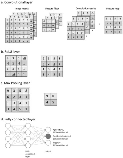
Figure 2.
CNN layer functions—(a) convolutional layer; (b) rectified linear unit layer; (c) max pooling layer and (d) fully connected layer.
- Convolutional layer performs the linear operation by doing element-wise multiplications and summations on every sub-input, using a group of weight matrixes called feature filters (Figure 2a). Feature filters learn their weights from training data; then each filter can detect the existence of a specific feature. The outputs are called feature maps. A feature map records not only the operation values but also the relative spatial location of these values. On the feature map, a higher output value indicates the potential existence of the corresponding feature at its relative location.
- Rectified linear units (ReLU) layer performs a nonlinear function (such as tanh and sigmoid) on the input (Figure 2b). Introducing nonlinearity to the system can improve computational efficiency without losing much accuracy. When performing a threshold operation: f(x) = max (0, x), where f is a nonlinear function applied to all values x in the matrixes, the negative values of input matrixes are rectified as 0 keeping the size of input volume unchanged.
- Pooling layer is a down-sampling layer (Figure 2c), aiming to decrease the size of the feature maps and to reduce the computational cost. A max pooling layer keeps only the maximal number of every sub-array (2 × 2) as the element of output array. Output omits unimportant features, while keeps the relative location of features.
- The fully connected layer multiplies the input by a weight matrix and then adds a bias vector to the output, an N-dimensional vector (Figure 2d). The output gives the probability of the input image belonging to each class, where N is the number of the category in a classification task.
2.2. Training and Testing of CNN
AlexNet, GoogLeNet and VGGNet were typical CNN architectures and were used in this study as the pre-trained models. AlexNet [9] consisted of 25 layers and had 62.3 million parameters such as the weight of every neuron insides layer plus bias. GoogLeNet was developed by Szegedy et al. [44], and it greatly reduced the number of parameters used in the network to 4 million, compared with 60 million typically used in AlexNet. VGGNet [29] can be regarded as a deeper AlexNet with 140 million parameters, so it used more computer memory and time to be fully trained. Initially, parameters were randomly generated and they were learnable through the training and testing process. The parameters of AlexNet, GoogLeNet, and VGGNet were adjusted through learning from millions of images.
Training of CNN can be performed by using supervised learning algorithms. Well-trained CNN models must learn from sufficiently labelled datasets so that the parameters could be greatly adjusted. Each training process of CNN consists of forwarding pass, loss function, backpropagation, and parameter update, and can be presented in the following six steps:
- Model initialization: all the parameters were randomly generated;
- Forward propagation: the input passed through the network layers and calculated the estimated output from the model;
- Loss function calculation: loss function was used to evaluate the prediction ability of the method. The most common loss function used the mean square error (E) between the model’s expected output and estimated output and can be formulated as follows:
The value of E decreased during the training process until reaching a constant that was used as a threshold for the next step. The objective of the training process was to minimize the loss function by feeding the network many inputs and the desired output;
- 4.
- Backpropagation: it is a process in which backward propagates the derivative of errors;
- 5.
- Parameters update: In general, the weights (parameters) update by the delta rules [45] was defined as follows:
New Weight = Old Weight − Derivative Rate × Learning Rate
If the deviation is positive, the parameter should be decreased; if the deviation is negative, the parameter should be increased; if the deviation equal to 0, then the parameter is optimal. The learning rate is a constant and should be set based on experience; if too small, it will take a long time to get optimal weights; if too large, the weights will deviate from optimal;
- 6.
- Iterates the process until convergence. Based on the previous step, the weights get updated very slowly, thus requesting many iterations to get the desired weights and minimize loss function. In reality, the CNN does not process the images one-at-a-time in order to increase productivity. A batch of samples is propagated through the network at the same time.
The labelled dataset from the same probability distribution as the training dataset [46] was split into training set and 30% for testing set, then the model was trained by the training set, after which the testing set was used for model evaluation. In classification task, the following indicators (Equations (3)–(5)) were used to access the performance of the classifier model:
where true positive (TN) were correctly identified, false positive (FP) were incorrectly identified, true negative (TN) were correctly rejected, and false negative (FN) were incorrectly rejected pixels.
The well-known pre-trained networks were trained by millions of images. For example, the GoogLeNet used 1.2 million images for training, 50,000 for validation and 100,000 images for testing, and it can classify 1000 categories of ground truth images. In reality, it is difficult to have datasets with sufficient size to train a complete network. Today, to complete an entire network from scratch, the training process can even take 2–3 weeks on multiple GPUs. Due to time restrictions or computational constraints in many researches, transfer learning becomes the first choice to apply DL methods, which allows a new task to be started by adopting a pre-trained network.
3. The Land Use Classification Method
3.2. Datasets for Transfer Learning
The UC-Merced Land Use Dataset contains 21-class high-resolution land-use images of the size of 256 × 256 pixels with 30 cm resolution. Examples of images are shown in Figure 3. Each category in the UC-Merced dataset has 100 images. These images were manually extracted from the USGS National Map Urban Area Imagery collection for various urban areas around the USA [23]. But countries and cities have a very different environment resulting in significant differences in architectural style and layout style, thus the classifications of the land-use. For example, most cities in China have very dense high-rise buildings and by contrast, most residential areas in the USA are characterized by sparse and much lower density, and downtown area in New York City has many high-rise buildings. Currently, there is a lack of a comprehensive dataset that includes land-use features sampled from different cities and countries. In the study area, agriculture, building and road network land-use classes were not similar with the images from the UC-Merced dataset based on the observation, so manually sampled images were used for these categories instead.
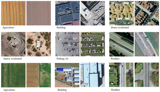
Figure 3.
Example images used for training the models—the UC-Merced dataset (the first two rows) and the manually extracted samples (the third row).
In order to address these varieties of possible land-use features and their classifications, this research used a mixture of the UC-Merced dataset and the manually sampled images from 2004 to 2017 digital orthophotos of the City of Surrey, BC, Canada. The size of the manually sampled images is 700 × 700 pixels and the resolution is 10 cm. The size of images from the UC-Merced dataset is 256 × 256 and the resolution is 30.5 cm. Therefore, the images from both sources cover almost the identical ground area. The manually sampled images were based on manual classification of features that represents agriculture, building and road network land-use classes.
The six main land-use classes used for classification and analysis were (1) green areas (GA); (2) industrial and commercial areas (In&Co); (3) high-density residential (HR); (4) low-density residential (LR); (5) parking lot (PL) and (6) road network (RN). For the purpose of model training and testing with 400 images for each LU class, the images were split randomly by the ratio of 70% (280 images) and 30% (120 images) with a total of 2520 and 1080 images for training and testing for each land-use, respectively.
3.3. Transfer Learning Strategies
There are three main options to apply transfer learning [47]. As shown in Figure 4, each option has different computational effort and accuracy. These options are as follows:
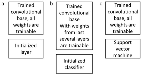
Figure 4.
Three different transfer learning scenarios—(a) fine-tuning the whole network; (b) fine-tuning higher layers of the network and (c) convolutional base as feature extractor.
- Fine-tuning the whole network (Figure 4a): Loading the pre-trained network, replacing the fully connected layer of the network, retraining the network using new dataset, and fine-tuning the weights of all layers through backpropagation.
- Fine-tuning the higher layers of the network (Figure 4b): Loading the pre-trained network, and freezing the parameters in the earlier layers of the network, so when retraining with new dataset, only the weights of last several layers will be updated.
- Convolutional base as a feature extractor and link a support vector machine (SVM) to form a CNN–SVM based model (Figure 4c): Loading the pre-trained network and feeding the data through the convolutional base; the output as the feature representations were then classified by SVM. This solution also required less computational effort.
4. Methodology
4.1. Study Area and Primary Data
The study area is a section of the community of Cloverdale, at the north-eastern part of the City of Surrey, Canada (Figure 5). The community of Cloverdale has been transformed over the years from a rural agricultural community to a prosperous small city attractive for young families, and it is known by its fast developing residential areas [48]; therefore, it was chosen as the suitable area to detect LU change through DL methods. The City of Surrey database provide orthophotos from 2004 to 2017, from which the LU classification was implemented. Since each orthophoto was large and took an average 4 h to classify, only the selected images of good quality were processed for simplicity reasons. Particularly, the orthophotos for years 2004, 2006, 2011, 2013, 2015 and 2017 were considered in order to document the LU change for the past 12 years. The digital orthophotos cover a section of the community of Cloverdale [49] with size 2.0 km × 3.6 km and with 10 cm spatial resolution. The 2011 land-use data from the Metro Vancouver Open Data Catalogue [50] and from DMTI Spatial Inc. [51] were also used as references.
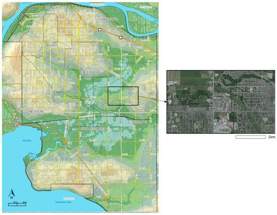
Figure 5.
Study area—north-east section of the Cloverdale, community of the City of Surrey, Canada [49,52].
4.2. Land Use Change Analysis
Figure 6 shows the process used to perform the land-use classification to identify the changes.

Figure 6.
Flowchart of the process for land-use change analysis based on the retrained CNN.
- The enriched UC-Merced dataset was used to fine-tune “GoogLeNet-‘pool5-drop’-SVM” models.
- The image of the study area was covering 20,000 × 36,000 pixels at a spatial resolution of 10 cm. The window with a pixel size of 700 × 700 shifted over and cropped the image in a specific order (from top to bottom and from left to right), with a stride of 100 pixels; therefore, there were {(20,000 − 700)/100 + 1} × {(36,000 − 700)/100 + 1} sub-patches, i.e., 194 × 354. The moving window covered all the image after 194 × 354 iterations with the same number of sequentially generated patches. These patches were sent to the classifier and land-use labels were returned. The numbers from 1 to 6 represent the six land-use labels. To extract the road network and green area land-use classes, the second process was repeated, while the size of moving window was set to 300 × 300 pixels, the matrix was only updated when the return label was 1 or 6. This process was done because green area and road network can exit in a small ground area independently. They can also become background of another feature if the moving window size was larger. For example, in a 700 × 700 pixels image, a small house can exist as agriculture land simultaneously, but the model will still think the image to be sparse residential. Therefore, the smaller window size, i.e. 300 × 300 pixels, was used again to separate out individual features from potentially misclassified 700 × 700 pixels images.
- A 194 × 354 void matrix was created; the cells in the matrix with index i corresponded to the ith image patches. The ith cell values were updated as the label number of the ith patch. Each cell represented a land-use category of a 10m spatial resolution for ground truth.
- The same classification method was applied to orthophotos for different years 2004, 2006, 2011, 2013, 2015 and 2017. Through the comparisons and statistical analyses of the obtained LU maps, the land-use change was quantified and analyzed.
5. Results and Discussion
The obtained values for total accuracy are given in Table 1 based on the eight transferred CNN-based models. The total accuracy was calculated using Equation (3). Models (a) and (b) were structured by fine-tuning the whole AlexNet and GoogLeNet, respectively; models (c) and (d) used ‘fc7’ or ‘fc6’ layer from AlexNet as feature extractor with SVM as a classifier; model (e) and (f) were based on the ‘loss classifier’ or ‘pool5-drop’ from GoogLeNet as feature extractor, respectively, with SVM as a classifier. Models (g) and (h) used, respectively, ‘fc7’ or ‘fc6’ from VGGNet as feature extractor and with SVM as a classifier.

Table 1.
The obtained values for the total accuracy of the eight transferred CNN-based models, where training and testing datasets were kept the same for each method.
Table 1 shows that the obtained values for model total accuracy from each transferred model rangeing from 95.1% to 98.1%. The transferred CNN models performed well on the land-use classification, with more than 95.0% accuracy. The accuracy difference was not large; however, the “GoogLeNet-‘pool5-drop’-SVM” classifier was chosen for further classification in the next step given its best performance on our training dataset. As an example, Figure 7 depicts the confusion matrix for the highest performing GoogLeNet-‘pool5-drop’-SVM. All the transferred models were trained on a single GPU ‘Quadro P2000’. The average computing time of models (a) and (b) were 45 min with single GPU, and models (c) to (h) took less than 5 minutes to generate classifier, which proved the time efficiency of using the transferred models, especially the CNN–SVM models.
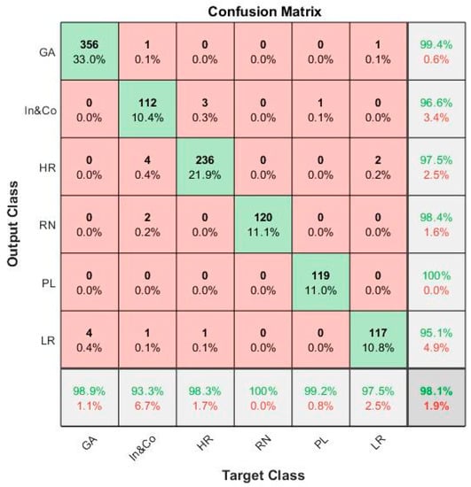
Figure 7.
Confusion matrix for the highest performing GoogLeNet-‘pool5-drop’-SVM. GA, green area; In&Co, industrial and commercial areas; HR, high-density residential areas; LR: low-density residential areas; PL: parking lot; RN: road network.
Figure 8 depicts the comparison of the obtained land-use classification map with the digital orthophoto of the study area in 2017. The boundary between different land-use classes was clearly defined in the resulting land-use map. Except for the north-western part of the study area, it can be seen that most of the remaining areas were classified as denser residential land-use. The middle of the study area was classified as industrial or commercial buildings’ land-use. The outline of major roads was distinct. Figure 8c presents the orthophoto image and the classified image of the track field at the north of the study area, indicating that the track field was fully occupied by cars. At the same location on the classified image, there was a black elliptical area at the south of the study area, which was labelled as a parking lot. Even though this elliptical area was misclassified, the model still demonstrated the sensitivity to capture the features of cars and the shape of the track field.
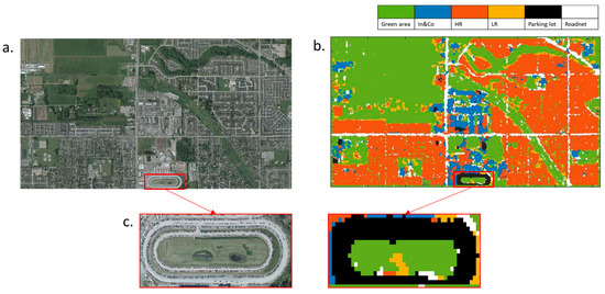
Figure 8.
(a) The orthophoto image of the study area with (b) the digital land-use map based on classification results for the year 2017. (1) Green area (GA), green color; (2) industrial and commercial areas (In&Co), blue color; (3) high-density residential areas (HR), red color; (4) low-density residential areas (LR), yellow color; (5) parking lot (PL), black color; (6) road network (RN), white color. (c) Detailed image of the zone with the field track filled with cars.
Based on the transferred “GoogLeNet-‘pool5-drop’-SVM” model trained by the enriched UC-Merced dataset, the land-use classification was performed for years 2004, 2006, 2011, 2013, 2015 and 2017 as shown in Figure 9. The composition result of land-use classes is given in Table 2, which shows that from 2004 to 2017, the green area decreased during urban development. Dense residential areas were increasing over the years and low-density residential areas were decreasing, as can be expected from the growing population [53] in this area. From 2006 to 2011, it can be seen that a new residential community appear at the north of the study area. The percentage of road network was decreasing, because the density of building and residential areas increased, which have occupied the road area. In 2017, the old track field at the north of the study area was used for parking. The parking lots are usually close to shopping malls and industrial buildings. These features can imply the location and number of industrial and commercial (In&Co) land-use class, which also increased, while the change was not significant. The overall results indicate that the community of Cloverdale tends to develop itself as a predominantly residential area and not as an industrial or agricultural area.
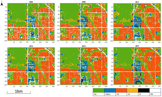
Figure 9.
Land use classifications obtained for years 2004, 2006, 2011, 2013, 2015 and 2017. GA, green area; In&Co, industrial and commercial areas; HR, high-density residential areas; LR, low-density residential areas; PL, parking lot; RN, road network.

Table 2.
Land use constitution of the study area from 2004, 2006, 2011, 2013, 2015 and 2017. GA, green area; In&Co, industrial and commercial areas; HR, high-density residential areas; LR, low-density residential areas; PL: parking lot; RN: road network.
Figure 10 presents the comparison of the obtained land-use classification with the reference land-use data for year 2011 [50,51]. The 2011 land-use map is the newest map the municipality has provided for public. Typically, the public land-use data for multiple years are difficult to obtain. They also contain different classifications that make their use challenging in computationally intensive data processing necessary for studies of land-use change process evolution over time. The 2011 land-use data (Figure 10b), from the Metro Vancouver Open Data Catalogue, contains more land-use types such as townhouse, high-rise building and institutional buildings, while land-use data for more recent years are not yet available. The land-use data from DMTI Spatial Inc. for the same year (Figure 10c) has lower thematic resolution and contains only the residential, open area, parks, and government institutional land-use classes. Due to the lack of high-quality land-use data and the orthophoto images, the proposed classification approach provides an economical solution for the LUC analysis.
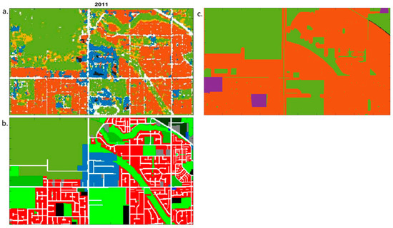
Figure 10.
Comparison of the land-use classifications for the year 2011 (a) resulting from the proposed CNN approach for the land-use classification; (b) from Metro Vancouver Open Data Catalogue [50] and (c) from DMTI Spatial Inc [51].
6. Conclusions
This research has focused on the (1) evaluation of eight transferred CNN-based models on land-use classification tasks, and (2) application of the best performing transferred CNN-based model as a classifier to classify and map the land-use from orthophotos of the study area. The results showed that successful land-use classification performance from all transferred models with at least 95.0% accuracy was obtained. The training and testing dataset that combined the off-the-shelf UC-Merced dataset with the manually classified images from the study area were used in order to enrich the data and train the model with the local land use features. Using the digital maps, the land-use change of the study area over years was interpreted.
The study has indicated the effectiveness of CNN-SVM models for land-use classification, especially with the “GoogLeNet-‘pool5-drop’-SVM” algorithm. The training data that was obtained from a real study area, including the manual image interpretation, can improve the overall classification results with significant time efficiency. Incorporating manual image interpretation makes the experiment less automatic, and it increases time for project completion. The proposed methodology requires selection and augmentation in every specific study area to reach better LU classification accuracy, which needs a little prior knowledge of the study area. Augmenting the amount of training datasets to cover wide variety of world regions will be helpful to improve classification and achieve higher accuracy using CNN models. Overall, the proposed land-use classification method can be transferred to analyze real-time digital orthophotos datasets from other urban–rural fringe areas, providing a fast and low-cost solution to aid land-use change analysis and to assist municipal land management.
Author Contributions
Data curation, C.C.; formal analysis, C.C., S.D. and S.L.; investigation, C.C. and S.D.; writing—original draft, review and editing, C.C. and S.D.; writing—review and editing, S.L.
Funding
This research was funded by Natural Sciences and Engineering Research Council (NSERC) of Canada Discovery Grants RGPIN-2017-03939 and RGPIN-2017-05950.
Acknowledgments
The authors are grateful for the full support of this study by Natural Sciences and Engineering Research Council (NSERC) of Canada Discovery Grants awarded to the second and third authors. The authors are thankful for the valuable comments and feedback of two anonymous reviewers.
Conflicts of Interest
The authors declare no conflict of interest.
References
- Zin, T.T.; Lin, J.C.-W. Big Data Analysis and Deep Learning Applications. In Proceedings of the First International Conference on Big Data Analysis and Deep Learning; Springer: Berlin, Germany, 2018. [Google Scholar]
- Progress towards the Sustainable Development Goals; N1713409; HLPF: New York, NY, USA, 2017.
- Foley, J.A.; DeFries, R.; Asner, G.P.; Barford, C.; Bonan, G.; Carpenter, S.R.; Chapin, F.S.; Coe, M.T.; Daily, G.C.; Gibbs, H.K.; et al. Global Consequences of Land Use. Science 2005, 309, 570–574. [Google Scholar] [CrossRef] [PubMed]
- Etingoff, K. Urban Land Use: Community-Based Planning; CRC Press: Boca Raton, FL, USA, 2017. [Google Scholar]
- Ienco, D.; Gaetano, R.; Dupaquier, C.; Maurel, P. Land Cover Classification via Multitemporal Spatial Data by Deep Recurrent Neural Networks. IEEE Geosci. Remote Sens. Lett. 2017, 14, 1685–1689. [Google Scholar] [CrossRef]
- Joseph, G. Fundamentals of Remote Sensing; Universities Press: Hyderabad, India, 2005. [Google Scholar]
- Arel, I.; Rose, D.C.; Karnowski, T.P. Deep Machine Learning—A New Frontier in Artificial Intelligence Research. IEEE Comput. Intell. Mag. 2010, 5, 13–18. [Google Scholar] [CrossRef]
- Liu, W.; Wang, Z.; Liu, X.; Zeng, N.; Liu, Y.; Alsaadi, F.E. A Survey of Deep Neural Network Architectures and Their Applications. Neurocomputing 2017, 234, 11–26. [Google Scholar] [CrossRef]
- Krizhevsky, A.; Sutskever, I.; Hinton, G.E. ImageNet Classification with Deep Convolutional Neural Networks. In Advances in Neural Information Processing Systems 25; Pereira, F., Burges, C.J.C., Bottou, L., Weinberger, K.Q., Eds.; Curran Associates, Inc.: Red Hook, NY, USA, 2012; pp. 1097–1105. [Google Scholar]
- LeCun, Y.; Boser, B.; Denker, J.S.; Henderson, D.; Howard, R.E.; Hubbard, W.; Jackel, L.D. Backpropagation Applied to Handwritten Zip Code Recognition. Neural Comput. 1989, 1, 541–551. [Google Scholar] [CrossRef]
- Hochreiter, S.; Schmidhuber, J. Long Short-Term Memory. Neural Comput. 1997, 9, 1735–1780. [Google Scholar] [CrossRef] [PubMed]
- Hinton, G.E.; Osindero, S.; Teh, Y.-W. A Fast Learning Algorithm for Deep Belief Nets. Neural Comput. 2006, 18, 1527–1554. [Google Scholar] [CrossRef] [PubMed]
- Vincent, P.; Larochelle, H.; Lajoie, I.; Bengio, Y.; Manzagol, P.A. Stacked Denoising Autoencoders: Learning Useful Representations in a Deep Network with a Local Denoising Criterion. J. Mach. Learn. Res. 2010, 11, 3371–3408. [Google Scholar]
- Lawrence, S.; Giles, C.L.; Tsoi, A.C.; Back, A.D. Face Recognition: A Convolutional Neural-Network Approach. IEEE Trans. Neural Netw. 1997, 8, 98–113. [Google Scholar] [CrossRef] [PubMed]
- Kalchbrenner, N.; Grefenstette, E.; Blunsom, P. A Convolutional Neural Network for Modelling Sentences. arXiv 2014, arXiv:1404.2188. [Google Scholar]
- Lu, Y.; Yi, S.; Zeng, N.; Liu, Y.; Zhang, Y. Identification of Rice Diseases Using Deep Convolutional Neural Networks. Neurocomputing 2017, 267, 378–384. [Google Scholar] [CrossRef]
- Nia, K.R.; Mori, G. Building Damage Assessment Using Deep Learning and Ground-Level Image Data. In Proceedings of the 2017 14th Conference on Computer and Robot Vision (CRV), Edmonton, AB, Canada, 16–19 May 2017; pp. 95–102. [Google Scholar] [CrossRef]
- Xu, G.; Zhu, X.; Fu, D.; Dong, J.; Xiao, X. Automatic Land Cover Classification of Geo-Tagged Field Photos by Deep Learning. Environ. Model. Softw. 2017, 91, 127–134. [Google Scholar] [CrossRef]
- Isikdogan, F.; Bovik, A.C.; Passalacqua, P. Surface Water Mapping by Deep Learning. IEEE J. Sel. Top. Appl. Earth Obs. Remote Sens. 2017, 10, 4909–4918. [Google Scholar] [CrossRef]
- Castelluccio, M.; Poggi, G.; Sansone, C.; Verdoliva, L. Land Use Classification in Remote Sensing Images by Convolutional Neural Networks. arXiv 2015, arXiv:1508.00092. [Google Scholar]
- Luus, F.P.S.; Salmon, B.P.; van den Bergh, F.; Maharaj, B.T.J. Multiview Deep Learning for Land-Use Classification. IEEE Geosci. Remote Sens. Lett. 2015, 12, 2448–2452. [Google Scholar] [CrossRef]
- Scott, G.J.; England, M.R.; Starms, W.A.; Marcum, R.A.; Davis, C.H. Training Deep Convolutional Neural Networks for Land-Cover Classification of High-Resolution Imagery. IEEE Geosci. Remote Sens. Lett. 2017, 14, 549–553. [Google Scholar] [CrossRef]
- Yang, Y.; Newsam, S. Bag-of-Visual-Words and Spatial Extensions for Land-Use Classification. In Proceedings of the 18th SIGSPATIAL International Conference on Advances in Geographic Information Systems, GIS ’10, San Jose, FL, USA, 2–5 November 2010; ACM: New York, NY, USA, 2010; pp. 270–279. [Google Scholar] [CrossRef]
- Hu, F.; Xia, G.S.; Hu, J.; Zhang, L.P. Transferring Deep Convolutional Neural Networks for the Scene Classification of High-Resolution Remote Sensing Imagery. Remote Sens. 2015, 7, 14680–14707. [Google Scholar] [CrossRef]
- Cheng, G.; Han, J.; Guo, L.; Liu, Z.; Bu, S.; Ren, J. Effective and Efficient Midlevel Visual Elements-Oriented Land-Use Classification Using VHR Remote Sensing Images. IEEE Trans. Geosci. Remote Sens. 2015, 53, 4238–4249. [Google Scholar] [CrossRef]
- Liu, Y.; Zhong, Y.; Fei, F.; Zhu, Q.; Qin, Q.; Liu, Y.; Zhong, Y.; Fei, F.; Zhu, Q.; Qin, Q. Scene Classification Based on a Deep Random-Scale Stretched Convolutional Neural Network. Remote Sens. 2018, 10, 444. [Google Scholar] [CrossRef]
- Nogueira, K.; Penatti, O.A.B.; dos Santos, J.A. Towards Better Exploiting Convolutional Neural Networks for Remote Sensing Scene Classification. Pattern Recognit. 2017, 61, 539–556. [Google Scholar] [CrossRef]
- Krizhevsky, A.; Sutskever, I.; Hinton, G.E. ImageNet Classification with Deep Convolutional Neural Networks. In Proceedings of the 25th International Conference on Neural Information Processing Systems—Volume 1, NIPS’12, Lake Tahoe, NV, USA, 3–6 December 2012; Curran Associates Inc.: Red Hook, NY, USA, 2012; pp. 1097–1105. [Google Scholar]
- Simonyan, K.; Zisserman, A. Very Deep Convolutional Networks for Large-Scale Image Recognition; ICLR: San Diego, CA, USA, 2015. [Google Scholar]
- Zhu, X.X.; Tuia, D.; Mou, L.; Xia, G.-S.; Zhang, L.; Xu, F.; Fraundorfer, F. Deep Learning in Remote Sensing: A Review. IEEE Geosci. Remote Sens. Mag. 2017, 5, 8–36. [Google Scholar] [CrossRef]
- Hughes, L.H.; Schmitt, M.; Mou, L.; Wang, Y.; Zhu, X.X. Identifying Corresponding Patches in SAR and Optical Images with a Pseudo-Siamese CNN. IEEE Geosci. Remote Sens. Lett. 2018, 15, 784–788. [Google Scholar] [CrossRef]
- Liu, Y.; Zhong, Y.; Fei, F.; Zhang, L. Scene Semantic Classification Based on Random-Scale Stretched Convolutional Neural Network for High-Spatial Resolution Remote Sensing Imagery. In Proceedings of the 2016 IEEE International Geoscience and Remote Sensing Symposium (IGARSS), Beijing, China, 10–15 July 2016; pp. 763–766. [Google Scholar] [CrossRef]
- Yao, Y.; Li, X.; Liu, X.; Liu, P.; Liang, Z.; Zhang, J.; Mai, K. Sensing Spatial Distribution of Urban Land Use by Integrating Points-of-Interest and Google Word2Vec Model. Int. J. Geogr. Inf. Sci. 2017, 31, 825–848. [Google Scholar] [CrossRef]
- Xia, G.-S.; Hu, J.; Hu, F.; Shi, B.; Bai, X.; Zhong, Y.; Zhang, L. AID: A Benchmark Dataset for Performance Evaluation of Aerial Scene Classification. IEEE Trans. Geosci. Remote Sens. 2017, 55, 3965–3981. [Google Scholar] [CrossRef]
- Oquab, M.; Bottou, L.; Laptev, I.; Sivic, J. Learning and Transferring Mid-Level Image Representations Using Convolutional Neural Networks. In Proceedings of the IEEE conference on computer vision and pattern recognition, Columbus, OH, USA, 23–28 June 2014; pp. 1717–1724. [Google Scholar]
- Romero, A.; Gatta, C.; Camps-Valls, G. Unsupervised Deep Feature Extraction for Remote Sensing Image Classification. IEEE Trans. Geosci. Remote Sens. 2016, 54, 1349–1362. [Google Scholar] [CrossRef]
- Zhou, B.; Lapedriza, A.; Khosla, A.; Oliva, A.; Torralba, A. Places: A 10 Million Image Database for Scene Recognition. IEEE Trans. Pattern Anal. Mach. Intell. 2018, 40, 1452–1464. [Google Scholar] [CrossRef] [PubMed]
- King, J.; Kishore, V.; Ranalli, F. Scene Classification with Convolutional Neural Networks; Course Project Reports 102; Stanford University: Stanford, CA, USA, 2017; p. 7. [Google Scholar]
- Razavian, A.S.; Azizpour, H.; Sullivan, J.; Carlsson, S. CNN Features Off-the-Shelf: An Astounding Baseline for Recognition. In Proceedings of the 2014 IEEE Conference on Computer Vision and Pattern Recognition Workshops, Columbus, OH, USA, 23–28 June 2014. [Google Scholar]
- Weng, Q.; Mao, Z.; Lin, J.; Guo, W. Land-Use Classification via Extreme Learning Classifier Based on Deep Convolutional Features. IEEE Geosci. Remote Sens. Lett. 2017, 14, 704–708. [Google Scholar] [CrossRef]
- Cloverdale. Available online: http://www.surrey.ca/community/6799.aspx (accessed on 20 January 2019).
- LeCun, Y.; Bengio, Y.; Hinton, G. Deep Learning. Nature 2015, 521, 436–444. [Google Scholar] [CrossRef] [PubMed]
- Bishop, C.M. Pattern Recognition and Machine Learning; Springer: New York, NY, USA, 2016. [Google Scholar]
- Szegedy, C.; Liu, W.; Jia, Y.; Sermanet, P.; Reed, S.; Anguelov, D.; Erhan, D.; Vanhoucke, V.; Rabinovich, A. Going Deeper with Convolutions. In Proceedings of the IEEE conference on computer vision and pattern recognition, Boston, MA, USA, 7–12 June 2015. [Google Scholar]
- Russell, I. The Delta Rule. Available online: http://uhaweb.hartford.edu/compsci/neural-networks-delta-rule.html (accessed on 21 December 2018).
- Ripley, B.D. Pattern Recognition and Neural Networks; Cambridge University Press: Cambridge, UK, 1996. [Google Scholar]
- Karpathy, A. CS231n Convolutional Neural Networks for Visual Recognition. Available online: http://cs231n.github.io/transfer-learning/ (accessed on 29 July 2018).
- City of Surrey. Available online: https://www.surrey.ca (accessed on 29 July 2018).
- City of Surrey’s Open Data. Available online: http://data.surrey.ca/ (accessed on 21 December 2018).
- Open Data Catalogue. Available online: http://www.metrovancouver.org/data (accessed on 21 December 2018).
- CanMap® GIS Data for GIS Mapping Software—DMTI Spatial. Available online: https://www.dmtispatial.com/canmap/ (accessed on 21 December 2018).
- City of Surrey Mapping Online System (COSMOS). Available online: http://cosmos.surrey.ca/external/ (accessed on 6 February 2019).
- Population Estimates & Projections. Available online: http://www.surrey.ca/business-economic-development/1418.aspx (accessed on 21 January 2019).
© 2019 by the authors. Licensee MDPI, Basel, Switzerland. This article is an open access article distributed under the terms and conditions of the Creative Commons Attribution (CC BY) license (http://creativecommons.org/licenses/by/4.0/).