CO₂ and CH₄ Emissions from Two Maar Crater Lakes (São Miguel, Azores)

Abstract

This study was made to quantify ΦCO₂ and ΦCH₄ in two crater monomictic lakes on São Miguel Island (Azores, Portugal). The studied water bodies are both within maar craters, with depths equal to 22 m and 33 m, at the Congro and Santiago lakes, respectively. ΦCO₂ values in both lakes are lower in summer, with a mean equal to 2.9 and 1.4 g m⁻² d⁻¹, respectively, in Congro and Santiago lakes, when the water column is stratified. ΦCH₄ displayed a different seasonal trend, with higher emissions during the period when the water column is stratified (mean value equal to 0.036 and 0.020 g m⁻² d⁻¹, respectively). Bacterial families commonly associated with CO₂ production, through heterotrophic respiration, fermentation, and syntrophic metabolism, were identified in both lakes, being the most abundant taxa Clostridiaceae, Enterobacteriaceae, Holophagaceae and Methylomonadaceae. The microbial community composition suggests seasonal variations, reflected by shifts in the relative abundance of specific microbial taxa. In particular, Clostridiaceae and Enterobacteriaceae exhibited higher relative abundance during winter, consistent with an increased contribution of fermentative microorganisms during this period. In contrast, Methylomonadaceae, a family commonly associated with methane oxidation and subsequent CO₂ production, reached higher relative abundance during summer in both lakes, suggesting enhanced methanotrophic activity during this period. Regarding CH₄ production, methanogens showed a slightly higher abundance during summer at Congro Lake, such as Methanosarcinaceae. In Santiago Lake, Syntrophaceae and unclassified Syntrophales were more abundant during summer, coinciding with higher CH₄ emissions compared to winter. The present research contributes to understanding volcanic gas release from lake water bodies in active volcanic framework, helping also to constrain GHG budgets in oceanic islands.

1. Introduction

In recent decades, surface water bodies have been recognized as significant natural emitters of carbon-based greenhouse gases (GHG), such as CO₂ and CH₄, thus contributing to global warming. Despite existing uncertainties, numerous estimates of global CO₂ flux (ΦCO₂; flux as the mass flow rate of a gas per a given area) from lakes have been proposed, starting with the landmark study of 1835 lakes by [1], which suggested a rate of 5.60 × 10² Tg CO₂ yr⁻¹, thus in the lower range of the later estimates by [2,3,4] varying from 5.83 × 10² to 1.4 × 10³ Tg CO₂ yr⁻¹. More recently, ref. [5] employed a size-productivity weighting method to estimate global ΦCO₂ from lakes to fall between 2.44 × 10² Tg CO₂ yr⁻¹ and 5.25 × 10² Tg CO₂ yr⁻¹, closer to the previous calculations by [1]. The lacustrine GHG emission is a function of several factors, such as, amongst others, depth [6], trophic state [7], and microbial activity, which plays a pivotal role in these emissions [8].

Methane flux (ΦCH₄) from surface water bodies has attracted increased scientific attention in recent years, following pioneering work by [9,10,11,12]. Despite some uncertainty, global estimates of CH₄ flux from different water bodies, such as lakes [13] and references therein, wetlands [14,15,16] and rivers [17], have been developed. Several studies suggested that after wetlands lake water bodies represent the second-largest aquatic source of methane, with various ΦCH₄ estimates ranging from 8 to 75 Tg CH₄ yr⁻¹ [10,13,14,18,19,20,21,22]. A more recent bottom-up assessment by [23], based on a dataset of 198 lakes, suggests a substantially higher mean global flux of 150.9 ± 73 Tg CH₄ yr⁻¹, representing approximately 37.9% of methane emissions from inland waters, and like inland wetlands (161 Tg CH₄ in 2020; [19]). Nevertheless, the median value of 55.8 Tg CH₄ yr⁻¹ from lake water bodies [23] falls clearly in the 8 to 75 Tg CH₄ yr⁻¹ range, highlighting the significant variability and ongoing uncertainty surrounding global lake methane flux estimates.

Recent studies have continued to emphasize the importance of lakes as significant natural sources of greenhouse gases, while also highlighting the large uncertainties that still exist in estimating global CO₂ and CH₄ emissions from inland waters [21,22]. However, most recent investigations have focused on global methane budgets, modeling approaches, or non-volcanic lake systems. Detailed hydrogeochemical studies integrating gas flux measurements, water chemistry, isotopic composition, and microbial communities in volcanic lakes remain scarce, emphasizing the need for further investigations in these unique environments.

With a total area of 2322 km², the Azores archipelago consists of nine volcanic islands located in the North Atlantic Ocean between 37° and 40° N latitude and 25° to 31° W longitude, at an approximate distance of 1500 km from Portugal mainland. The mean annual precipitation (1930 mm yr⁻¹) is much higher than the mean actual evapotranspiration (581 mm yr⁻¹), implying a high runoff (~3.22 × 10⁸ m³ yr⁻¹; [24]). Moreover, a water volume of about 1.1 × 10⁸ m³ is stored in the 88 surface lakes spread in the Azores, namely at the São Miguel, Terceira, Pico, Flores, and Corvo islands [24,25,26], 50% of which occupy the bottom of volcanic explosive craters and 16.7% lay down in the floor of subsidence calderas [27]. Two other lakes are located inside lava caves in Graciosa and Terceira islands [27], highlighting the diverse volcanic geomorphology along the Azores archipelago and its influence on surface water distribution. Considering only volcanic lakes, ΦCO₂ were estimated at 32 ± 5.2 Tg CO₂ yr⁻¹, 80% of which were of magmatic origin [28]. No comprehensive global assessments are available for ΦCH₄ from volcanic lakes; however, CH₄ is known to be only a minor component in geothermal and volcanic emissions worldwide compared to CO₂ [29].

In the Azores archipelago, recent research has advanced quantification of CO₂ emissions from volcanic lakes. Building on several studies made in the last decade [30,31,32,33,34,35,36], CO₂ emissions from the surface of a dataset made by 45 volcanic lakes in the Azores was estimated as ~171 × 10³ t CO₂ yr⁻¹, from which 42% is of volcanic origin (~72 × 10³ t CO₂ yr⁻¹; [37]). In contrast, methane emissions from lakes in the Azores remain largely unquantified. To the date, the first study about methane dynamics is by [38], which addressed the mechanisms that are regulating CH₄ release from five lakes spread on São Miguel Island (Sete Cidades, Santiago, Fogo, Congro, and Furnas), followed by research made with the objective of estimate the combined ΦCH₄ and ΦCO₂ in Capitão and Caiado lakes, both on Pico Island [39], and Caldeirão lake (Corvo Island; [40]).

The present study aims to quantify ΦCO₂ and ΦCH₄ from two maar crater lakes on São Miguel Island (Azores archipelago), through accumulation chamber measurements made at the surface of the water bodies, coupled by an overall hydrogeochemistry characterization, and to identify the main drivers that controls these GHG emissions. It is expected that our data will contribute to a more accurate quantification of GHG emissions from water bodies in active volcanic areas, thus allowing to better constraining the GHG balances. Studies of this type, that examine the combined emission of CO₂ and CH₄ from lakes situated within active volcanic structures, are innovative in international literature, given that typically only CO₂ emissions have been characterized in such environments.

2. Study Area

2.1. Geological Setting

2.1.1. Congro Lake

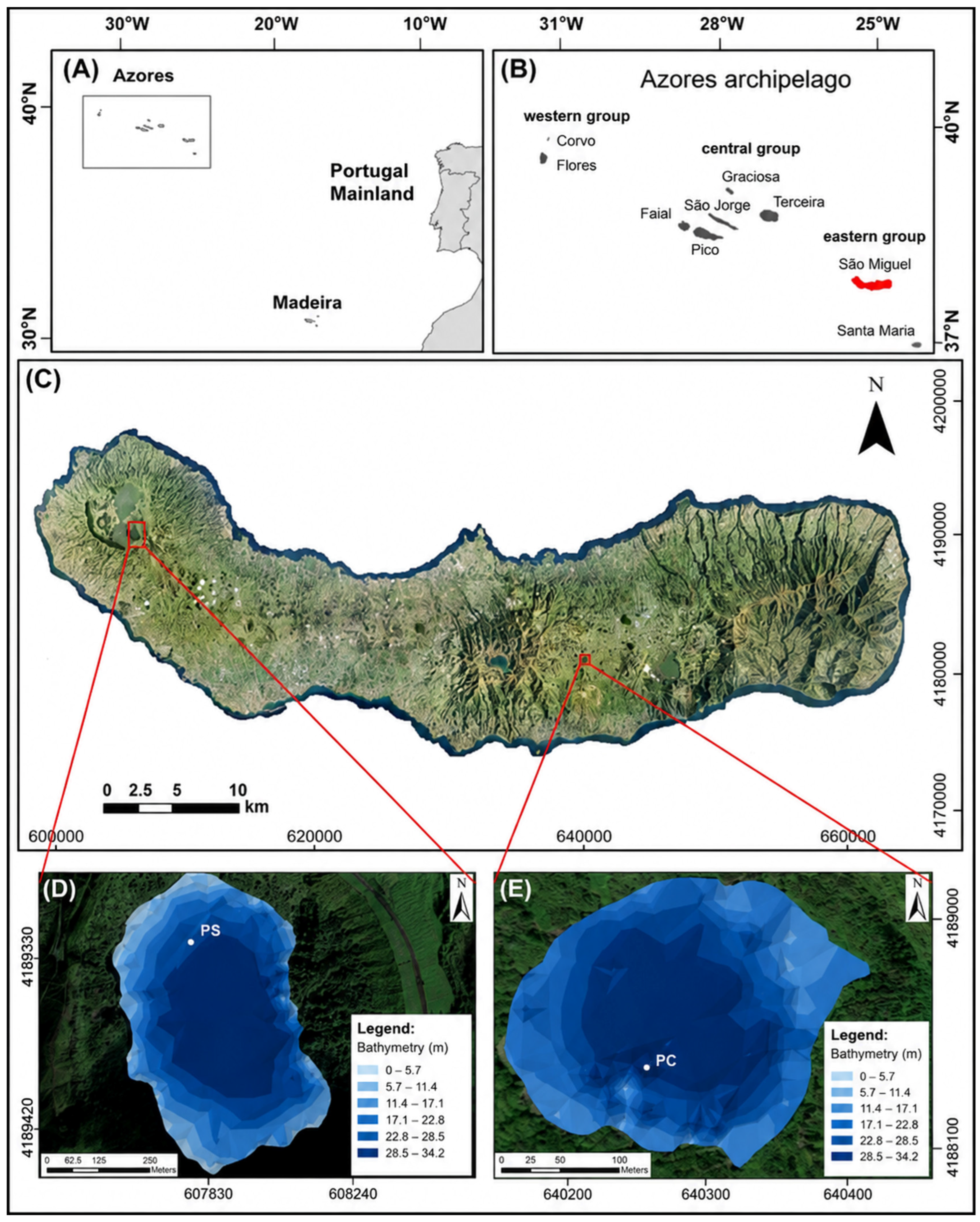
Congro Lake is located in the SW quadrant of the Congro Fissural Volcanic System, the easternmost of the two active fissural systems of São Miguel, located in the central part of the island between Fogo and Furnas central volcanoes (Figure 1A–C). It corresponds to a flat-topped elevated area (≥500 m a.s.l. in the central zone) extending for about 8 km in an E–W direction, with gentle slopes towards the coastal cliffs. This fissural system is predominately punctuated by scoria cones, but pumice cones, domes, and maars are also present [41].

The Congro Lake maar is a volcanic structure associated with the last period of activity of the Congro Fissural Volcanic System. Congro volcanism appears to have been most significant between 30 kyr and 10 kyr [42] and characterized by effusive or low-explosivity basaltic activity. Some of the lava flowed eastward, infilling the Furnas caldera. Volcanic activity remained important between 10 kyr and 5 kyr and was largely dominated by basaltic fissure-type eruptions, producing lava that inundated the entire area and reached the north and south coasts. Eruptions of more evolved magma were of minor significance. Volcanism gradually decreased up to ~5 kyr, when it almost over. The two most recent eruptions were centered on Congro Lake area. The first was a trachytic eruption (Congro maar eruption) which included extrusion of domes and explosive phreatomagmatic activity. The second eruption was basaltic and formed a scoria cone north of Congro maar. The entire volcanic field is mantled by thick pumice fall deposits from the recent eruptions of Fogo and Furnas volcanoes [40,43].

The maar is located at the intersection of two volcano-tectonic structures, one with NNE-SSW direction and the other with NW-SE direction, corresponding to a broad crater with steep-sided walls and a diameter of approximately 500 m. The Congro maar eruption, dated at 3800 ± 400 years BP [44], started with the extrusion of a trachytic dome, which was partially destroyed by the explosive episode that formed the maar. The final phase of the eruption involved the extrusion of another small dome that occupies part of the crater. The associated deposit is lithic-rich and well-stratified, with alternating beds of trachytic coarse-grained pumice and fine-grained ash. The explosive phreatomagmatic event corresponds to a Volcanic Explosivity Index (VEI) of 3 (eruption volume of 0.08 km³) [43].

2.1.2. Santiago Lake

Santiago Lake is one of the several lakes present in the Sete Cidades volcanic edifice, the westernmost of the three active central volcanoes of São Miguel. It is located on the SE sector of the caldera and occupies the crater of a deep maar with steep-sided walls, measuring 1.1 km by 0.8 km across. The Santiago Lake maar is located at the intersection of the regional NW–SE-oriented faults associated with the SE extension of Mosteiros Graben and an inferred arcuate or ring fault inside the caldera.

Sete Cidades has a broadly circular caldera with a diameter of approximately 5 km and sub-vertical inner walls some 30 to 400 m high. The floor of the caldera is occupied by several volcanic features, such as pumice cones, tuff rings/cones, domes, maars and craters, with the latter being filled by perennial lakes. The outer flanks of the volcano increase gradually in slope from the coastal cliffs up to the caldera rim. The most common volcanic features on the flanks are scoria cones, either isolated or forming ridges, although a few domes are also found on the western flank [45,46]. The volcanostratigraphy of Sete Cidades is organized into two main groups that reflect important events or changes in eruptive history [46,47]. The Inferior Group includes all products related to the subaerial construction of the volcanic edifice (or shield-building stage), ranging from >210 kyr to ~36 kyr, and was characterized mainly by effusive or low-explosivity volcanism. The Superior Group comprises products younger than 36 ka and represents the onset of the caldera formation. This latter period was marked by three paroxysmal eruptions, namely at 36 ka (Risco Formation), 29 kyr (Bretanha Formation), and 16 kyr (Santa Bárbara Formation), all related to the different phases of formation of the caldera. In the last 5 ka, at least 17 trachytic explosive eruptions, predominantly hydromagmatic, occurred inside the caldera (P1 to P17), and several basaltic eruptions (>12) occurred on the flanks of the volcano. The products of the recent eruptions constitute the Pepom Member [45,46,47].

The maar of Santiago Lake is a volcanic structure associated with the most recent period of activity of Sete Cidades Volcano. It is thought that this maar corresponds to the vent of the P8 trachytic explosive eruption, dated at 2659 ± 55 years (²²⁶Ra/²³⁰Th maximum age; [48]). The associated deposit is very well-stratified and composed of pumice lapilli and ash fall layers rich in lithics, resulting from an oscillatory eruption of alternating hydromagmatic and magmatic activity, with a Volcanic Explosivity Index (VEI) of 4 (eruption volume of 0.12 km³) [45].

2.2. Hydrological Setting

Congro and Santiago lakes are lying at an altitude of about 400 m a.s.l., and the main characteristics of these water bodies are presented in Table S1 (Supplementary Material). Congro Lake has a surface area of 4.4 × 10⁻² km² and a maximum depth of 22 m, as measured during the present study. In contrast, Santiago Lake is both larger and deeper, with a surface area of 2.5 × 10⁻¹ km² and a maximum depth of 33 m. Based on storage volumes of 5.8 × 10⁵ m³ for Congro and 5.3 × 10⁶ m³ for Santiago, and assuming runoff inflow as the only water input (8 × 10⁴ m³ yr⁻¹ for Congro and 2.17 × 10⁵ m³ yr⁻¹ for Santiago; [26]), the estimated residence times are approximately 7.2 yr and 24.5 yr. As no spring discharges or artificial outlets have been identified along the lakes margins, and the relatively small lake surface areas limit the contribution of rainfall, the main source of uncertainty in the residence time estimates is groundwater seepage through the lake floor. These water bodies are currently classified as having poor ecological status according to WFD criteria [26], mainly due to ongoing eutrophication processes.

3. Methodology

3.1. General Water Chemistry

Water chemistry in both lakes was characterized along four surveys, two of which made in the winter period (1st survey—March 2023; 4th survey—December 2023), and the remaining in the summer period (2nd survey—June 2023; 3rd survey—September 2023). The somehow narrow observation window of the present study may limit conclusions on the seasonal dynamics, both for water chemistry and for GHG emissions and microbial community composition. Since both lakes have monomictic nature, the summer and winter surveys allow to characterize any variations under contrasting fully mixed and stratified conditions. Water samples were collected at every two meters depth intervals along vertical profiles, made in each lake at the maximum depth location (locations PS and PC, in Santiago and Congro lakes; Figure 1D,E), using a 1 L-capacity SEBA sampling bottle. A total of 93 samples has been collected, 37 at Congro Lake (9 in all surveys except for the 2nd survey—10 samples), and 56 at Santiago Lake (12—1st survey; 15—2nd survey; 14—3rd survey; 15—4th survey).

Immediately following sample collection, pH, temperature, and electrical conductivity (EC) were determined in situ using a portable multiparameter instrument (WTW Multi 3620 IDS, Xylem Analytics Germany Sales GmbH & Co. KG, Weilheim, Germany). Titrations for the determination of alkalinity and dissolved carbon dioxide contents were also made in the field following standard procedures [49], using NaOH (1/44 M) and H₂SO₄ (0.05 M) solutions as titrants until pH value reach a value of 8.3 and 4.45, respectively. Despite the uncertainties associated with these titrations, dissolved CO₂ values were only used to check the respective pattern along the water column, while the alkalinity was used for the computation of the bicarbonate content, allowing a further description of the water types in both lakes.

Major-ion composition was determined in the hydrogeochemisty laboratory of the Research Institute for Volcanology and Risk Assessment (University of the Azores), using atomic absorption spectrometry equipment (GBC 906AA, GBC Scientific Equipment Pty Ltd., Melbourne, Australia) for cations (Na⁺, K⁺, Mg²⁺, Ca²⁺), and ionic chromatography for anions (Thermo Fisher Dionex Integrion HPIC, Thermo Fisher Scientific, Waltham, MA, USA). In both cases, samples were filtered in the field using 0.2-μm filters (cellulose acetate) and kept in polyethylene bottles, and for atomic absorption spectrometry they were also acidified with suprapur nitric acid.

Two samples were also collected in each lake to proceed with the characterization of the δ¹³C-DIC stable isotopic ratio, at the surface and at the bottom of the water column, mainly to determine if a deep-seated C-source influences water chemistry. Sample collection took place at the same location as the vertical profiles (PS and PC), during the 1st survey, and was made according to the procedure defined by the International Atomic Energy Agency [50]. Samples were processed in a 60 L plastic container with a stirrer, connected to a wide mouthed plastic bottle of 1 L capacity screwed in the bottom, in which the precipitate will settle after adding the reagents. Firstly, the pH of the sample was raised to about 11, through the addition of 50 mL of carbonate-free concentrated NaOH, and after 5 g of iron sulphate (Fe₂O₁₂S₃·nH₂O) and about 150 g of BaCl₂ were also stirred into the sample. The velocity of the precipitate formation was accelerated by adding about 40 mL of Praestol solution to the sample. After the precipitation is fully achieved, the bottom bottle may be removed from the apparatus to collect the precipitate. All along the process, exposure to the atmosphere is prevented to avoid atmospheric CO₂ contamination.

Stable isotope analyses were performed at the Stable Isotope Laboratory of the Estación Biológica de Doñana (CSIC, Spain) using a continuous-flow isotope ratio mass spectrometry (CF-IRMS) system (Thermo Electron, Bremen, Germany). The analytical setup consisted of a Flash HT Plus elemental analyzer (Thermo Fisher Scientific, Bremen, Germany) coupled to a Delta V Advantage (Thermo Fisher Scientific, Bremen, Germany) isotope ratio mass spectrometer. The analytical precision was better than ±0.15‰.

3.2. Diffuse CO₂ Flux

CO₂ flux measurements were performed using portable equipment based on the accumulation chamber method [51], adapted to allow fluctuation [52]. This approach has been previously applied in studies conducted in the Azores [30,31,37]. The accumulation chamber technique allows us to measure the rate of CO₂ increase within a chamber placed at the surface of the lake, inside which the gas is continuously pumped to an infrared detector and returned. The flux itself is then calculated as the increase in CO₂ during a certain period in a chamber of a known volume. Chamber measurements can provide meaningful results, being a simple and low-cost method. Despite some concerns, some studies have shown that chamber measurements are close to values obtained with other approaches [53]. Moreover, this method has been shown to provide reliable measurements under low to moderate wind conditions, with wind speeds below approximately 8 to 10 m s⁻¹; [54], a threshold much higher that wind speed observed along the present study.

The portable system was equipped with an infrared LI-COR LI-820 CO₂ detector (LI-COR Biosciences, Lincoln, NE, USA), with a maximum range of 20,000 ppm and capable of measuring CO₂ fluxes from 0 to 30,000 g m⁻² d⁻¹ [55]. CO₂ flux measurements were performed at the lake surface on the same days as water sampling. At each node of the measurement grid, the chamber was deployed once for approximately 60–120 s, resulting in 65 and 100 measurements in Congro Lake (surveys 1 and 2, respectively) and 173 and 140 measurements in Santiago Lake. The measurement grids covered approximately 0.05 km² in Congro Lake and 0.27 km² in Santiago Lake, following a near-uniform spatial distribution. The relatively small size of the lakes allowed all measurements to be completed within a short time period, minimizing potential uncertainties associated with temporal variations in CO₂ fluxes throughout the day. The geographic coordinates of each measurement point were recorded, together with water depth measurements obtained using a Garmin ECHOM™ 500c bathymetric probe (Garmin Ltd., Olathe, KS, USA). Since near-surface turbulence and gas transfer velocities are strongly influenced by atmospheric conditions [56], wind speed was monitored at 5 min intervals during field surveys using a portable weather station (PCE FWS 20N, PCE Instruments, Meschede, Germany) installed on the lake shore. Ambient air temperature was also recorded with the same instrument.

The Graphical Statistical Approach (GSA), e.g., [51], and the sequential Gaussian simulation (sGs) [57] were applied to data, allowing a further comparison of results; both methodologies were already applied in a previous study in the same area [31]. Graphical statistical analysis (GSA), based on cumulative probability plots, was applied to identify distinct data populations, background values, and anomalous thresholds [58]. The presence of different lognormal populations may indicate contributions from separate CO₂ sources, such as biogenic and volcanic-hydrothermal inputs [30,37,51,57,59]. Besides the identification of different lognormal populations, GSA enables the determination of their mean and standard deviation, as well as the respective proportion [58]. A T-Sichel estimator [60] was used to calculate population means and their 95% confidence interval.

The sGs application followed the algorithm described by [61] to characterize the spatial distribution of CO₂ fluxes and generate degassing maps. The original data was transformed into a normal distribution using a normal score transformation [57,61], enabling the application of the multi-Gaussian distribution required by the method. Experimental variograms were then calculated to define the spatial structure of each dataset and used in the sGs procedure to generate 100 realizations of the flux grid using Wingslib software (version 1.5; [61]).

Total diffuse CO₂ emissions were estimated by integrating the mean flux values obtained from the sGs simulations over the lake surface area. This approach was based on E-type maps, which represent the expected flux at each location through the point-wise average of all realizations [57]. This methodology was applied in studies related to CO₂ spatial analysis in volcanic regions, e.g., [62] and references therein.

3.3. Methane Flux Measurements

3.3.1. Empirical Measurements

The value of ΦCH₄ were determined in both lakes using static floating chambers (SFC) arranged several transects. Each transect comprised six SFCs spaced at regular intervals along a straight line and attached to a cable to prevent drifting. Gas samples from the chambers were collected at periodic intervals to measure the increase in concentration as a function of time inside a receptacle of known geometry [63], namely three and thirty minutes after SFC deployment at the lake surface. Wind speed was also measured at each 5 min-interval using the same equipment as for CO₂ flux determinations, assuring steady ambient conditions to prevent near-surface turbulence.

Non-steady-state chambers are commonly used for measuring ΦCH₄ from the earth surface to the atmosphere [64] and references therein. Compared to the floating accumulation chamber used for CO₂ measurements, that enables integration of the gas build-up inside the chamber, being the gas pumped to an infrared detector, SFC uses a somewhat similar buoyant container to measure gas concentration enclosed inside, but in this case sampling is discrete, followed by analytical determination in the laboratory. Despite not being quantified in the present study, some uncertainties on the flux measurements are associated with these methods, resulting from the chamber design itself, such as the aspect ratio (volume/area), and ambient conditions [65]. Nevertheless, floating chambers are very useful, especially when conditions are logistically demanding, such as the ones of the present study [66]. Consequently, the whole-lake methane emission estimates derived from these measurements should be regarded as preliminary and interpreted accordingly.

The SFC consisted of HDPE bucket bottoms cut to a diameter of 40 cm and a height of 14 cm, mounted within inflated tire inner tubes that served as floating bases. The containers were tightly fitted into the inner tubes to prevent air leakage. When deployed at the lake surface, 2–3 cm of the inner tube remained submerged, ensuring an airtight seal and preventing atmospheric air from entering the chamber. A three-way valve installed at the upper section of each container enabled gas sampling while maintaining chamber integrity. The valve remained closed except during sampling, when it was connected to a syringe. Gas samples were subsequently transferred into 12 mL glass vials fitted with screw caps and pierceable rubber septa using a two-needle system. Before sampling procedure, vials were filled with slightly acidified (pH ~4) deionized water to minimize CO₂ dissolution, which is expelled during sample injection.

At Congro Lake, CH₄ flux measurements took place along the 3rd and the 4th surveys, comprising 3 (17 SFC measurements) and 6 transects (36 SFC measurements), respectively. At Santiago, the total number of transects is equal to 2 (12 SFC measurements) and 7 (42 SFC measurements), respectively. The transects were made in locations selected to assure representativeness, a procedure to which the results of the previous measurements that took place in the 3rd were also instrumental. Samples were collected at each SFC along the transect at 3 and 30 min after placement in water. Water physico-chemical parameters, including temperature, pH, dissolved O₂, water depth, as well as air temperature, were measured concurrently with gas sampling. Gas samples were analyzed by gas-chromatography at the Department of Earth Sciences (University of Florence, Italy), using a Shimazu 14A gas chromatograph (Shimadzu Corporation, Kyoto, Japan) equipped with a flame ionization detector and a 10 m long stainless-steel column packed with Chromosorb PAW 80/100 mesh.

Using the CH₄ concentrations in each vial, flux calculations followed Equation (1) [67]:

$$\mathsf{\Phi }C{H}_4={\displaystyle \frac{dC{H}_4}{dt}}\times {\displaystyle \frac{V}{A}},$$

(1)

where

dCH₄/dt, increment of the CH₄ concentration inside the chamber;

V, volume of the SFC receptacle;

A, basal area of the SFC receptacle.

3.3.2. Diffuse Methane Flux Calculations

Water samples were collected at each SFC location in 30 mL glass vials, avoiding air bubbles during sampling. Helium was added to create a headspace for dissolved gas equilibration, and the gas composition was subsequently analyzed by gas chromatography at the Department of Earth Sciences, University of Florence (Italy), using a Shimadzu 15A instrument (Shimadzu Corporation, Kyoto, Japan) equipped with a 5 m stainless-steel column packed with Chromosorb PAW 80/100 mesh and a thermal conductivity detector.

The CH₄ diffusive flux at the water-air interface was calculated from the measured dissolved concentration using the thin boundary layer model (TBL; [68]), that follows Equation (2):

$${\varphi }_{{CH}_4}=k_{{CH}_4}\left(C_{{CH}_4,w}-C_{{CH}_4,eq}\right),$$

(2)

where

$C_{{CH}_4,w}$, measured dissolved CH₄ concentration;

$C_{{CH}_4,eq}$, calculated dissolved CH₄ concentration;

$k_{{CH}_4}$, gas transfer velocity.

The calculated gas concentration was estimated considering equilibrium with the atmosphere, according to gas solubilities as function of temperature and salinity.

Gas transfer velocity is computed through Equation (3):

$$k_{{CH}_4}=k_{600,{CH}_4}\times {\left({\displaystyle \frac{S_{C_{CH4}}}{600}}\right)}^x,$$

(3)

where:

$k_{600,{CH}_4}$, corresponding to the kCH₄ normalized to 600;

$S_{C_{CH4}}$, Schmidt number, computed as function of temperature according to the fourth order polynomial [69];

$x$, value selected as function of the roughness of the water surface, according to the wind speed (−0.67 for wind speed lower than 3 m s⁻¹; −0.5 if wind speed is higher than 3 m s⁻¹).

The $k_{600,{CH}_4}$ values were calculated based on local wind speed (considered as equal to 2 m s⁻¹), following Equation (4) proposed by [70]:

$$k_{{600,CH}_4}=0.72\times U_{10},$$

(4)

where:

$U_{10}$, wind speed at a height of 10 m.

3.4. Sediment Sampling and DNA Extraction

Sediment samples were collected from sites PS and PC, respectively, in the Santiago and Congro water bodies (Figure 1D,E) using a UWITEC© gravity corer (90 mm internal diameter; UWITEC GmbH, Mondsee, Austria) to depths of 20–40 cm. The upper 2 cm of each core were transferred to sterile plastic bags for microbial analyses, transported to the laboratory under cool, dark conditions, and stored at −80 °C until processing. Total DNA was extracted from 250 mg of sediment using the DNeasy PowerSoil Pro Kit (QIAGEN, Hilden, Germany). DNA extracted from three subsamples of each homogenized core was pooled, and their concentration was measured using the Qubit™ dsDNA HS/BR Assay Kits (Invitrogen, Thermo Fisher Scientific, Waltham, MA, USA).

Full-length 16S rRNA gene sequencing was performed on the PacBio SMRT third-generation platform using the universal primers 27F (AGRGTTYGATYMTGGCTCAG) and 1492R (RGYTACCTTGTTACGACTT), each carrying a sample-specific PacBio barcode. Amplicons were generated using the KAPA SYBR FAST qPCR Kit, (Roche Sequencing Solutions, Pleasanton, CA, USA), pooled at equimolar concentrations, prepared with the SMRTbell Express Template Prep Kit 2.0 (Pacific Biosciences, Menlo Park, CA, USA). Sequencing was performed using the Sequel II Sequencing Kit 2.0 (Pacific Biosciences, Menlo Park, CA, USA).

Raw sequencing reads were quality-filtered and screened for chimeras using the MOTHUR pipeline. High-quality reads were clustered into operational taxonomic units (OTUs) and taxonomically assigned against the SILVA 138 database. Alpha diversity was assessed using species richness and Shannon diversity indices, while beta diversity was evaluated by principal coordinates analysis (PCoA) based on Bray–Curtis dissimilarity. Community compositional differences were statistically checked using permutational multivariate analysis of variance (PERMANOVA), and differential abundance analysis was performed to identify taxa showing significant spatial or seasonal variation. Statistical analyses were made in RStudio (RStudio Team, Boston, MA, USA) running version 4.5.1 using the ‘vegan’ and ‘DESeq2’ packages.

4. Results

4.1. Lake Water Chemistry

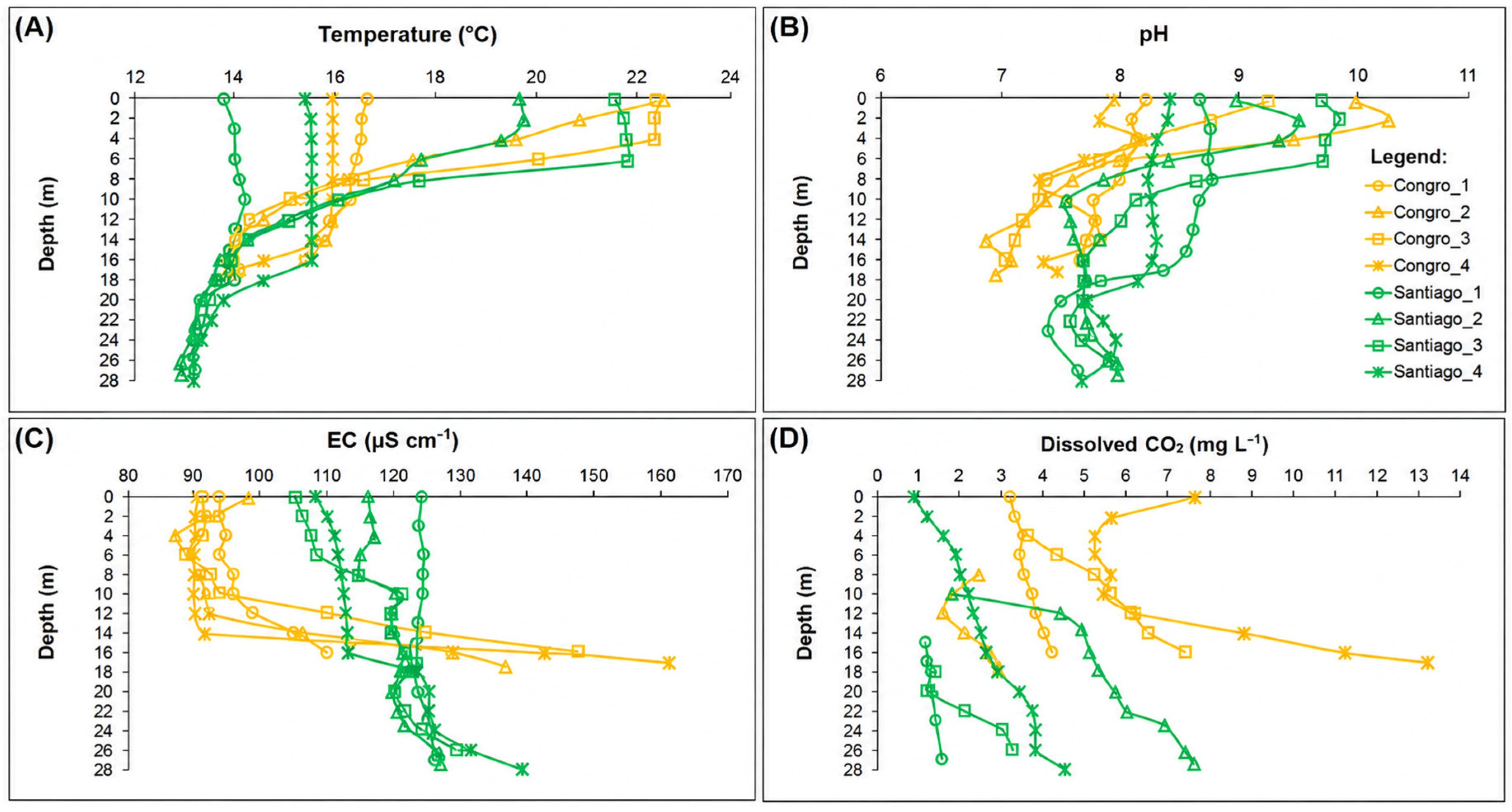
Descriptive statistics of the physico-chemical and major-ion composition of the collected samples are presented in Table S2 (Supplementary Material; Congro Lake) and Table S3 (Supplementary Material; Santiago Lake). Water temperature is in the range between 13.8 °C and 22.5 °C (mean = 16.7 ± 2.6 °C) for the entire Congro dataset, varying between 12.9 °C and 21.8 °C (mean = 15.3 ± 2.5 °C) for Santiago Lake. During the 2nd and the 3rd surveys, conducted during summer, under conditions of thermal stratification, the difference between the surface and bottom layers reached 8.7 °C and 8.8 °C in the Congro and Santiago lakes, respectively. Instead, during the 1st and 4th surveys, made in winter, when conditions favor mixing, the difference does not exceed 1.0 °C to 1.5 °C (Figure 2A).

The pH ranged between 6.88 and 10.26 (mean = 7.88 ± 0.80) for the Congro dataset, while for Santiago the pH ranged between 7.41 and 9.86 (mean = 8.23 ± 0.65). Pronounced vertical pH gradients were observed during periods of stratification in the summer months, during which surface pH reached values as high as 10.26 and 9.85, respectively, at the Congro and Santiago lakes (Figure 2B).

EC is slightly higher in Santiago Lake relative to Congro Lake, with values for all dataset ranging between 105 and 139 µS cm⁻¹ (mean = 119 ± 7 µS cm⁻¹) in the former, and between 87 and 161 µS cm⁻¹ (mean = 100 ± 17 µS cm⁻¹) in the latter (Figure 2C). Values are also higher at the bottom of the lakes relative to the (Figure 2C), suggesting solute accumulation at depth during stratification periods. At the bottom there is a slight dissolved CO₂ enrichment, mainly when the water column is stratified, reaching values as high as 7.4 mg L⁻¹ (3rd survey on Congro Lake) and 7.6 mg L⁻¹ (2nd survey on Santiago Lake) in these conditions (Figure 2D).

Waters are predominantly from the Na-HCO₃ type in both lakes, besides some samples from Congro Lake that are from the Na-HCO₃-Cl type (Figure S1—Supplementary Material). The water chemistry in both lakes expresses the influence of the main processes that drive water composition, namely sea salts deposition and water–rock interaction, which are consistent with findings from previous studies [27,71].

4.2. CO₂ Diffuse Flux

ΦCO₂ measurements made at Congro Lake along the 1st survey (March 2023) ranged between 2.2 and 12.1 g m⁻² d⁻¹ (mean = 6.4 ± 2.3 g m⁻² d⁻¹; median = 6.0 g m⁻² d⁻¹), and along the 2nd survey (June 2023) ranged between 0 and 14.6 g m⁻² d⁻¹ (mean = 2.9 ± 2.6 g m⁻² d⁻¹; median = 2.7 g m⁻² d⁻¹) (

Table 1. Descriptive statistics of ΦCO₂ in the studied lakes according to the sampling survey (n, number of measurements). Surveys were made respectively during winter (1st measurement survey—March of 2023) and summer (2nd measurement survey—June of 2023).

Lake	Survey	n	Min. (g m−2 d−1)	Max. (g m−2 d−1)	Mean ± SD (g m−2 d−1)	Median (g m−2 d−1)
Congro	1	65	2.2	12.1	6.4 ± 2.3	6.0
	2	100	0.0	14.6	2.9 ± 2.6	2.7
Santiago	1	173	2.7	14.4	7.2 ± 2.0	7.2
	2	140	0.0	5.9	1.4 ± 1.7	0.6

; Figure S2A,B—Supplementary Material). For Santiago Lake, values ranged between 2.7 and 14.4 g m⁻² d⁻¹ (mean = 7.2 ± 2.0 g m⁻² d⁻¹; median = 7.2 g m⁻² d⁻¹) and between 0 and 5.9 g m⁻² d⁻¹ (mean = 1.4 ± 1.7 g m⁻² d⁻¹; median = 0.6 g m⁻² d⁻¹), respectively (Table 1; Figure S2C,D—Supplementary Material). Mean values for ΦCO₂ flux in both lakes are like the ones measured in a previous work [31].

Through the cumulative probability plots the differences between the measurement surveys are also depicted. During the 1st survey a single lognormal population is to be seen in both lakes, pointing out to a sole CO₂ source, corresponding to low flux values, as high as 14.4 g m⁻² d⁻¹) (Figure S3A,C—Supplementary Material). Instead, three populations are identified during the 2nd survey, and besides population A, that corresponds to null values, population B and C correspond to low values, in the range of 0.24 to 2.3 g m⁻² d⁻¹ and of 1.7 to 14.6 g m⁻² d⁻¹, respectively (Figure S3B,D—Supplementary Material). Measurements are lower than the background value of 35 g m⁻² d⁻¹, a reference threshold derived for Furnas Volcano and above which a deep-seated CO₂-source also contributes to the overall flux [30].

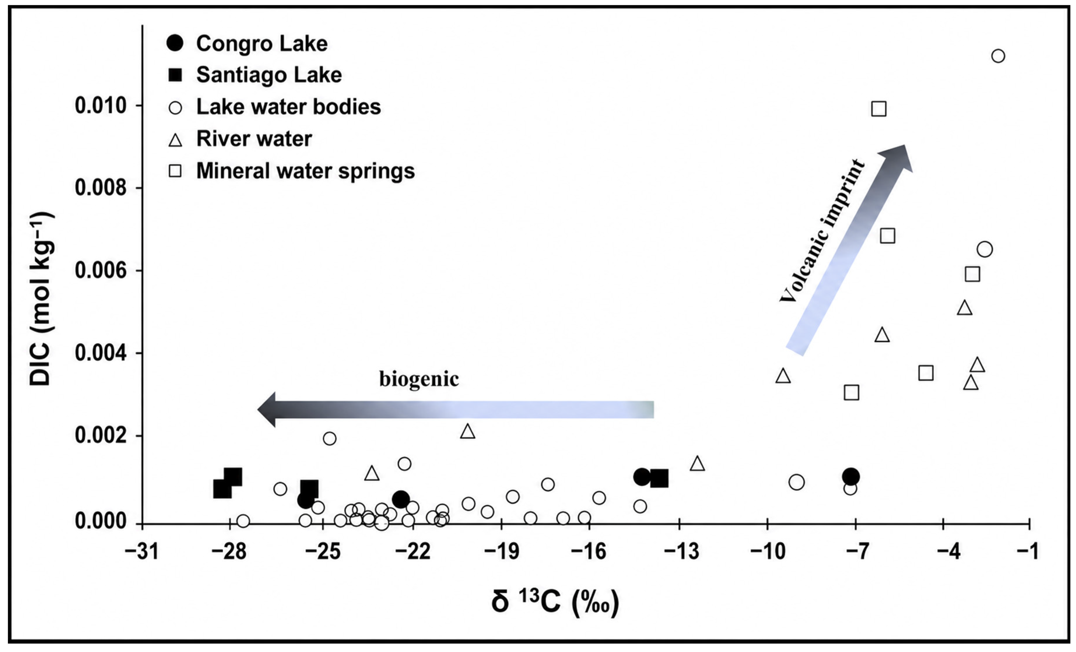
The δ¹³C-DIC values also suggest a biogenic source as the samples collected are in the range of −7.21‰ to −28.37‰ (mean = −20.65‰ ± 7.90‰), and therefore have lighter compositions relative to the range for mantle CO₂ (−3.5 to −6‰; [72]) (Figure 3). One of the samples collected at the bottom of Congro Lake presented a value equal to −7.21‰, and was thus heavier than the typical δ¹³Corg but close to the ¹³C composition of today’s atmosphere (~−8.3‰; [73]). This value is also heavier than measurements made along a previous study, and it is suggested that some sort of atmospheric contamination took place during sampling procedures.

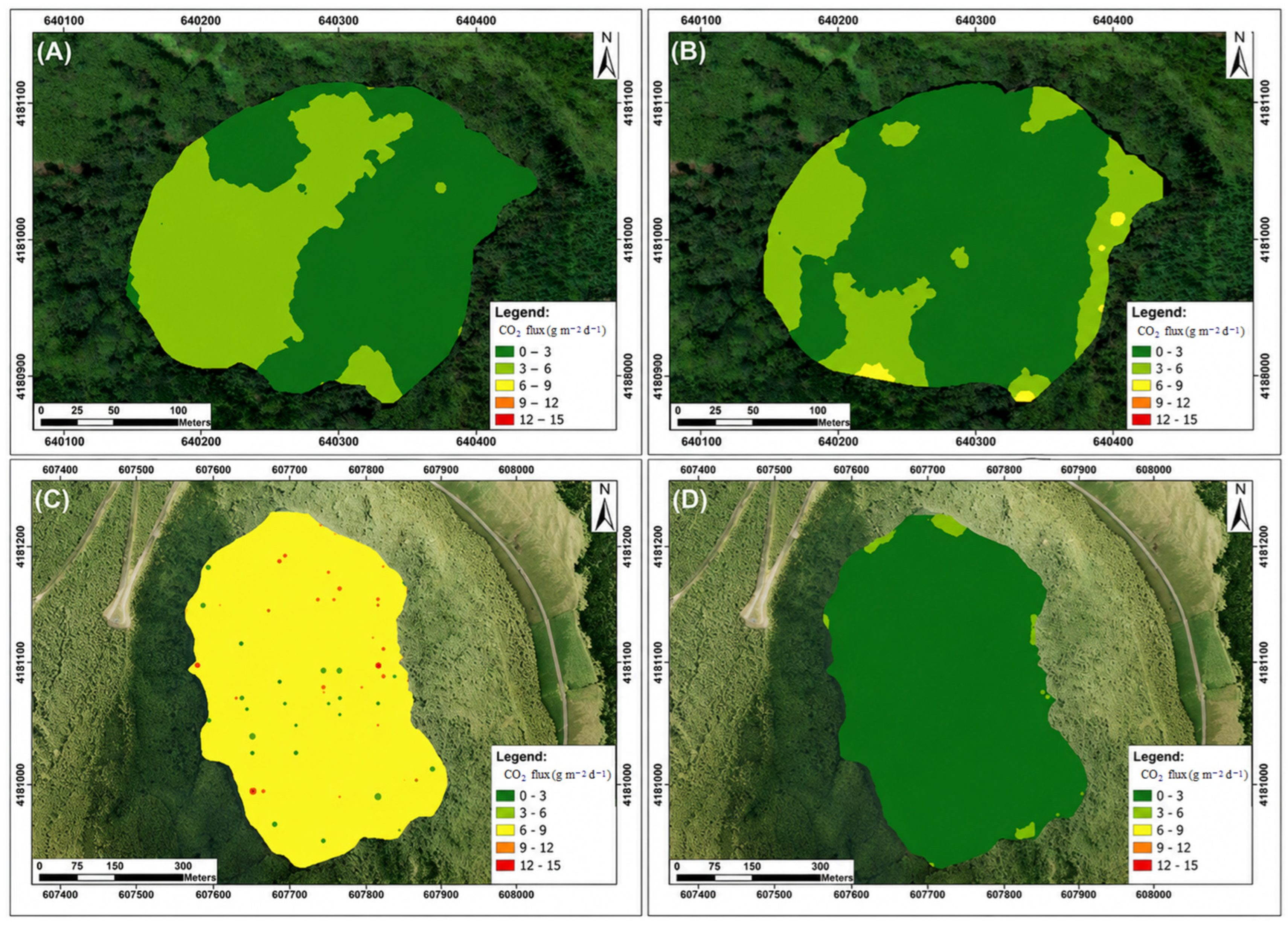
Modeled variograms show that data follows a spherical structure, presenting nugget values in the range of 0.4 to 0.65 and 0.36 to 0.85, respectively for Congro and Santiago lakes (Figure S4). The influence of each measured point relative to neighboring values ranged between 55 and 103 m for Congro Lake (Figure S4A,B—Supplementary Material), and from 95 to 290 m at Santiago Lake (Figure S4C,D—Supplementary Material). Through 100 equiprobable sGs simulations over the respective datasets, average CO₂ flux maps were made for the surveys on both lakes (Figure 4). The spatial distribution of values reflects the monomictic character of the studied lakes, with higher CO₂ fluxes recorded in winter, during periods of complete water column mixing, compared to periods characterized by stratified hydrological conditions (Figure 4A–D). During the summer stratification period, the higher CO₂ flux values are predominantly observed near the lake margins, where the water depth is much lower (Figure 4D). This pattern suggests that physical and thermal gradients associated with stratification, combined with topographical variations in the lake bathymetry, significantly influences the spatial distribution of CO₂ emissions, in agreement with previous studies [30,31].

4.3. CH₄ Diffuse Flux

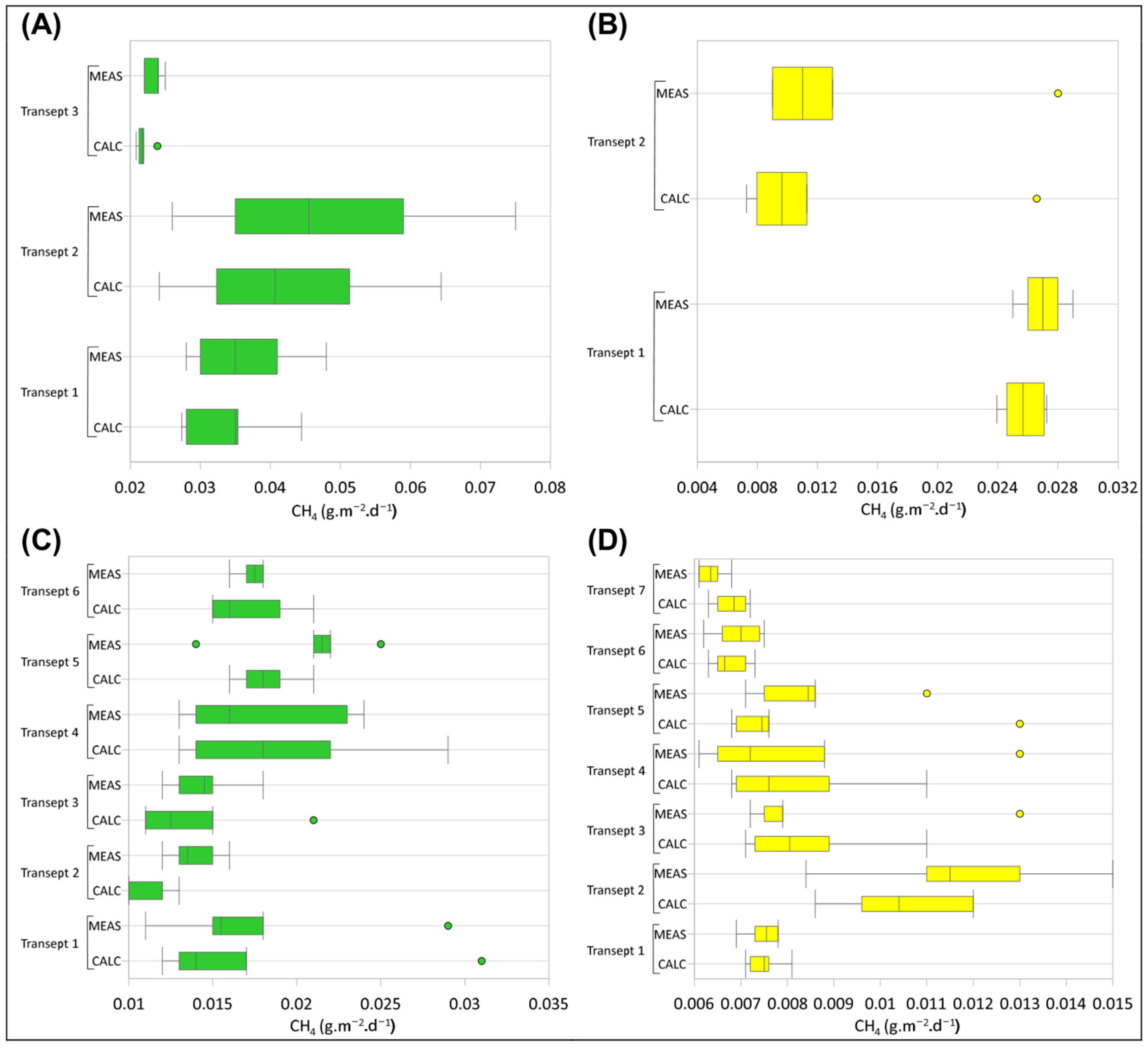
Results for both measured and calculated ΦCH₄ for the several transects made in both surveys are shown in Tables S4 and S5 (Supplementary Material). The theoretical estimates made using the TBL model closely aligned to the measured values, suggesting the robustness of the field survey methodology (Figure 5). A similar outcome was reported by [67], who applied a comparable SFC-based field approach. In this latter study, field measurements were compared with values calculated through three different methods, and the better theoretical approximation was the one that estimates $k_{600,{CH}_4}$ following the expression by [70]. Because ebullition was not accounted for in the present study, and given that it is frequently the dominant pathway for methane emissions from surface water bodies [23], the reported CH₄ release estimates may represent a conservative assessment and are likely underestimated. Therefore, the reported CH₄ fluxes and consequently the whole-lake methane emission estimates should be regarded as preliminary.

The measured methane emission along the two surveys range between 0.022 and 0.075 g m⁻² d⁻¹ (mean = 0.036 ± 0.015 g m⁻² d⁻¹; median = 0.035 g m⁻² d⁻¹), and between 0.011 and 0.029 g m⁻² d⁻¹ (mean = 0.017 ± 0.004 g m⁻² d⁻¹; median = 0.016 g m⁻² d⁻¹) at Congro Lake, respectively (

Table 2. Descriptive statistics of ΦCH₄ in the studied lakes according to the sampling survey (n, number of measurements). Surveys were made, respectively, during summer (3rd measurement survey—September of 2023) and summer (4th measurement survey—December of 2023).

Lake	Survey	n	Type	Min. (g m−2 d−1)	Max. (g m−2 d−1)	Mean ± SD (g m−2 d−1)	Median (g m−2 d−1)
Congro	3	17	Meas	0.022	0.075	0.036 ± 0.015	0.035
			Calc	0.021	0.064	0.033 ± 0.012	0.032
	4	36	Meas	0.011	0.029	0.017 ± 0.004	0.016
			Calc	0.010	0.031	0.016 ± 0.005	0.015
Santiago	3	12	Meas	0.009	0.029	0.020 ± 0.009	0.026
			Calc	0.007	0.027	0.019 ± 0.009	0.024
	4	42	Meas	0.006	0.015	0.008 ± 0.002	0.008
			Calc	0.006	0.013	0.008 ± 0.002	0.007

). The interquartile range (IQR) is higher for the 3rd survey (0.016 g m⁻² d⁻¹) compared to the 4th survey (0.004 g m⁻² d⁻¹).

In the case of Santiago Lake, values measured along the two surveys range between 0.009 and 0.029 g m⁻² d⁻¹ (mean = 0.020 ± 0.009 g m⁻² d⁻¹; median = 0.026 g m⁻² d⁻¹), and between 0.006 and 0.015 g m⁻² d⁻¹ (mean = 0.008 ± 0.002 g m⁻² d⁻¹; median = 0.008 g m⁻² d⁻¹), respectively. As observed also with the Congro values, the IQR in the Santiago dataset is higher for the 3rd survey (0.016 g m⁻² d⁻¹) compared to the 4th survey (0.002 g m⁻² d⁻¹), showing a larger dispersion of data in the former survey, reflecting increased spatial and temporal variability under stratified conditions.

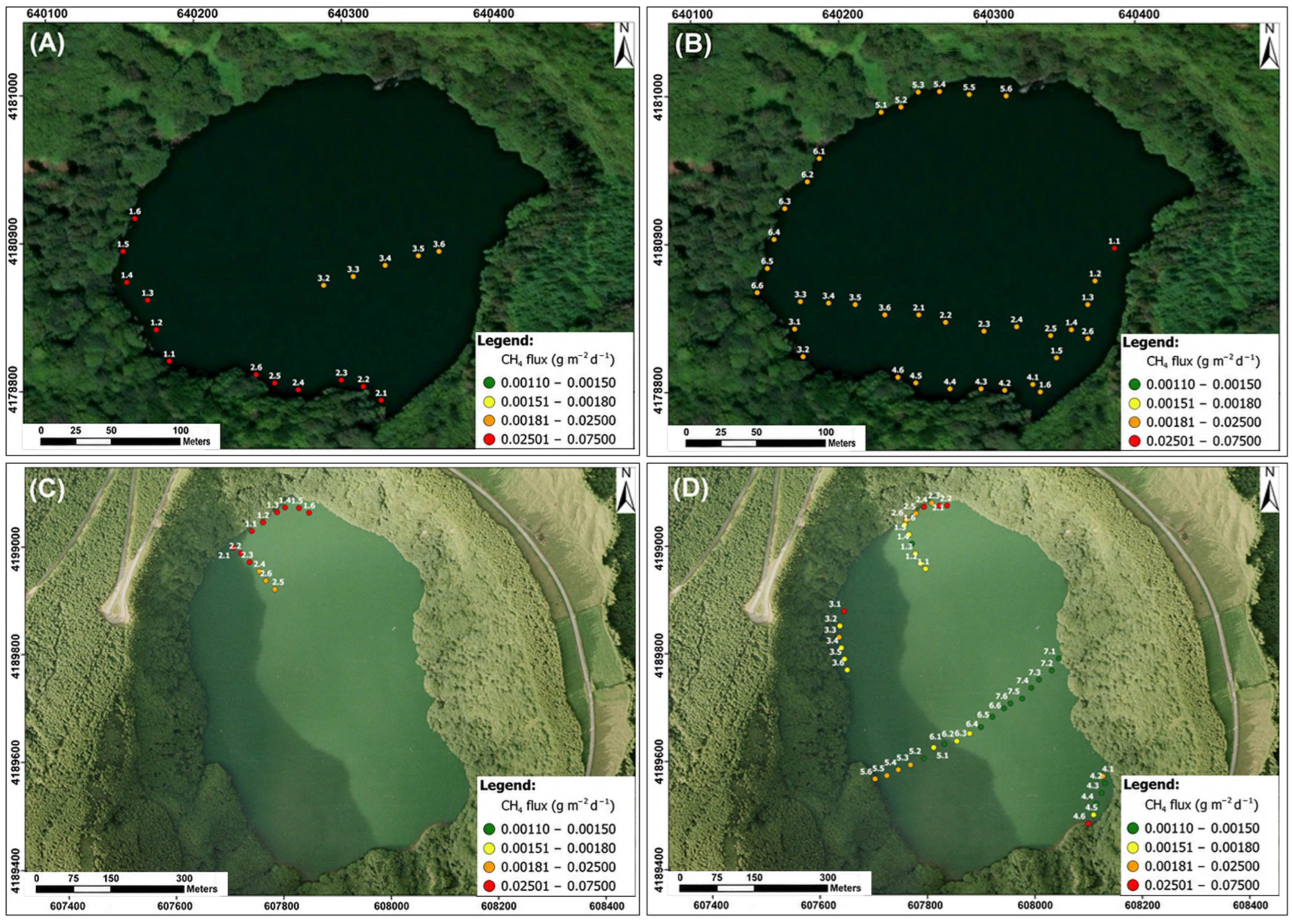
This variability aligns with previous findings suggesting that dissolved CH₄ content in lakes can fluctuate significantly over space and time [75]. The spatial distribution of the measured CH₄ flux along the Congro and Santiago lakes also reflects this dynamic behavior. Other studies made worldwide highlighted substantial interannual variability in methane fluxes, even larger than the median diel variability [10,76].

4.4. Microbial Community and Seasonal Variations

The microbial community structure characterization was based on 12 samples collected across both lakes and seasons, and sequencing yielded 28,456 high-quality reads per sample after quality filtering. Microbial diversity and evenness revealed clear differences between lakes and sampling: the Alpha diversity analysis ranged from 1423 in Congro Lake, during summer, to 3695 in Santiago, during winter. The Shannon diversity index was higher in Santiago, reaching 6.54 in winter, while Congro exhibited lower diversity, with a minimum of 1.89 during summer. Simpson’s index indicated greater community evenness in Santiago during winter (0.991), compared to Congro in summer (0.571). These patterns suggest a pronounced seasonal effect on microbial community composition, with higher diversity and richness in winter, the significance of which will be further discussed (Table S6—Supplementary Material). The rarefaction curves showed that the sequencing depth was sufficient to capture microbial diversity across all samples, as the curves approached saturation, suggesting that most of the microbial diversity present in the sediments was detected (Figure S5—Supplementary Material).

The microbial communities in both lakes displayed distinct taxonomic compositions, with variations which seem to be influenced by seasonal and spatial factors. Analysis of the full-length 16S rRNA gene sequences identified Proteobacteria, Firmicutes, Bacteroidetes, and Actinobacteria as the dominant phyla across all samples (Figure S6—Supplementary Material). Proteobacteria predominated in both lakes, particularly in Santiago during winter, while Firmicutes were more abundant in Congro, especially in winter, suggesting enhanced organic matter degradation during this period.

In Santiago Lake, winter samples showed increased representation of Rhodocyclaceae and Nitrosomonadaceae, taxa associated with nitrogen cycling. In Congro, winter communities were enriched with Clostridiaceae and Syntrophomonadaceae, known for their role in anaerobic decomposition. Summer samples on Santiago Lake were marked by a higher abundance of Methylomonadaceae, while on those Congro Lake exhibited an increase in Holophagaceae and Prolixibacteraceae.

Non-Metric Multidimensional Scaling (NMDS) analysis supported these observations, revealing distinct clustering of microbial communities between the two lakes and clear seasonal separation within each lake (Figure S7—Supplementary Material), even though the period studied somewhat limits more in-depth conclusions regarding seasonal behavior. The stratification observed suggests that both lakes undergo dynamic seasonal shifts, potentially driven by variations in temperature, nutrient availability, and organic matter input.

By analyzing the microbial taxa directly associated with carbon cycling, specifically CO₂ and CH₄ production, it is possible to show a seasonal shift in the relative abundance of key bacterial groups involved in fermentation, methanogenesis, and methane oxidation, whose relative abundance was associated with the observed seasonal patterns of ΦCO₂ and ΦCH₄ (Tables S7 and S8—Supplementary Material). Bacterial families associated with CO₂ production include those involved in heterotrophic respiration, fermentation, and syntrophic metabolism, were identified in both lakes, the most abundant taxa being Clostridiaceae and Enterobacteriaceae, the ones presenting much higher OTUs during winter, as well as Holophagaceae, and Methylomonadaceae (Table S7—Supplementary Material). The bacterial families involved in methane production are shown in Table S8 (Supplementary Material), with higher abundances of Methanobacteriaceae, Syntrophaceae, Syntrophorhabdaceae, Desulfovibrionaceae and Anaerolineaceae during summer.

5. Discussion

5.1. ΦCO₂ and ΦCH₄ Seasonal Patterns

As previously pointed out, ΦCO₂ values are higher along the 1st survey (March 2023) comparing to the 2nd survey (June 2023; Figure S2—Supplementary Material). This release is consistent with the seasonal mixing behavior of monomictic lakes, where CO₂ builds up in deeper, anoxic layers during stratification and is subsequently released during turnover events. The dissolved CO₂ enrichment observed during the summer period at the bottom of the water column, when stratification takes place, also results from this hydrological behavior (Figure 2D). In these periods, thermal stratification limits vertical mixing, allowing CO₂ to accumulate in the hypolimnion until mixing resumes in cooler seasons.

In contrast, ΦCH₄ displayed a different seasonal trend along the studied period, with higher emissions during the 3rd survey (September 2023), despite a smaller number of transects, comparing to the 4th survey (December 2023). The 3rd survey made in both lakes, that comprised CH₄ flux measurements, was made in summer, during which the water column was stratified, while the second set of SFC transects was made in winter when full mixing conditions prevail, reflecting the monomictic character of the water bodies (Figure 6). Another study, made in a much larger but shallower lake, has also found a similar temporal pattern, with higher CH₄ emissions during summer [77]. The seasonal variance of temperature plays also a significant role in enhancing methane production from sediments [78]. Elevated summer temperatures appear to stimulate microbial methanogenesis, particularly in shallow zones where sediment–water interactions are more pronounced. In fact, in areas with depths of less than 5 m, ΦCH4 were substantially higher during the summer surveys compared to winter. In Congro Lake mean CH₄ emissions reached 0.0588 g m⁻² d⁻¹ in summer, compared to 0.0195 g m⁻² d⁻¹ in winter. Similarly, in Santiago Lake, values are also higher during summer (0.0278 g m⁻² d⁻¹) compared to winter (0.0112 g m⁻² d⁻¹). This suggested seasonal increase aligns with previous findings demonstrating that methane production rates are positively correlated with temperature [79], and the effect of this driver was shown, for example, in [80].

Projected climate warming could further amplify this effect. For example, the expected rise in water temperature in lakes estimated in average as between 0.86 and 2.60 °C may imply an increase in methane production rates of about 13% to 40% by the end of the century [81]. These projections highlight the potential for volcanic lakes, such as Congro and Santiago, to become increasingly significant contributors to atmospheric methane emissions under future warming scenarios. Although this study did not investigate aerobic methane production, its potential contribution to CH₄ emissions cannot be excluded. Previous research on São Miguel Island lakes has documented methane production in oxic conditions, particularly in the epilimnion [38]. This process is associated with microorganisms capable of metabolizing methylated compounds, which may contribute to methane production within the water column [82]. The microbial CH₄ production, known as the methane paradox, has been reported in other aquatic ecosystems [83,84].

5.2. Influence of Microbial Communities over the ΦCO₂ and ΦCH₄

In the studied lakes, the microbial community exhibited clear seasonal changes, with a substantial increase in the relative abundance of some of the dominant taxa during winter. For example, the relative abundance of Clostridiaceae increased from 0 to 262 OTUs in Congro, and from 0 to 30 OTUs in Santiago Lake (Table S7—Supplementary Material). Similarly, Enterobacteriaceae increased from 4 to 944 OTUs, and from 4 to 35 OTUs, respectively, indicating intensified fermentation during colder months. This seasonal microbial dynamic was associated with distinct gas flux patterns recorded in both lakes. Higher ΦCO₂ values were observed during winter, reaching 6.4 g m⁻² d⁻¹ in Congro and 7.2 g m⁻² d⁻¹ in Santiago, coinciding with the higher abundance of fermentative bacteria taxa. Although these microorganisms are known to participate in carbon cycling under low-oxygen conditions, the present dataset only supports an association between microbial composition and gas fluxes and does not allow a direct causal relationship to be established at the whole-lake scale. Nevertheless, this pattern is consistent with observations from other eutrophic lake systems, where fermentative bacteria have been identified as important contributors to carbon dioxide production under low-oxygen conditions [7,12].

In contrast, Methylomonadaceae, responsible for methane oxidation and subsequent CO₂ production, peaked during summer, in both lakes, but particularly in Congro, where abundance increased from 29 in winter to 88 in summer, suggesting active methanotrophic activity during this period. Summer samples on Santiago Lake were marked by a slightly higher abundance of Methylomonadaceae, while on Congro Lake also exhibited an increase in Smithellaceae, suggesting shifts in organic matter utilization.

Methane production is suggested to be predominantly mediated by methanogenic archaea and syntrophic bacteria, which are usually involved in the breakdown of complex organic substrates into methanogenic precursors and syntrophic bacteria, the most relevant taxa being Methanobacteriaceae, Syntrophaceae, Syntrophorhabdaceae, and Desulfovibrionaceae (Table S8—Supplementary Material). At Congro Lake, methanogens showed slightly increased abundance during summer, with Methanosarcinaceae increasing from 120 to 140 OTUs, suggesting enhanced acetate availability in warmer months. This coincided with a marked increase in Desulfovibrionaceae, from 1 to 223 OTUs, indicating intensified sulfate-reducing activity, a process that may compete with methanogenesis for available substrates. At Santiago Lake, summer was characterized by an increase in Syntrophorhabdaceae from 10 to 20 OTUs, suggesting that syntrophic activity contributes to CH₄ production. In contrast, Syntrophaceae decreased from 11 OTUs, in winter, to 2 OTUs, in summer, suggesting a seasonal shift in the composition of syntrophic consortia. These variations were observed together with higher CH₄ emissions during summer compared to winter, suggesting a potential association between seasonal microbial community shifts and methane emissions. However, the present results do not demonstrate that these microbial groups directly controlled the observed whole-lake CH₄ fluxes.

This higher abundance of methanogenic archaea observed during the warmer months coincided with the higher ΦCH₄ values measured in both lakes, with Congro Lake exhibiting a threefold increase from 0.0195 to 0.0588 g m⁻² d⁻¹ and Santiago Lake showing an increase from 0.0112 to 0.0278 g m⁻² d⁻¹. This seasonal pattern may be associated with environmental conditions that are more favorable for methanogenesis, including higher temperatures and increased organic matter decomposition under stratified conditions. However, the present data only support an association between microbial community composition and methane fluxes and do not demonstrate that the abundance of methanogenic archaea directly controlled the measured whole-lake CH₄ emissions. Likewise, despite the higher abundance of methanotrophic bacteria such as Methylomonadaceae, which are known to oxidize methane and contribute to CO₂ production, their specific influence on the observed gas fluxes cannot be directly inferred from the current dataset. Similar seasonal dynamics have been documented in temperate lakes, where temperature-driven stratification and reduced methane oxidation have been associated with enhanced methane flux during warmer months [85]. Furthermore, the NMDS results revealed distinct clustering of microbial communities according to both lake and season, supporting the existence of seasonal shifts in microbial community composition. While these observations are consistent with the current understanding of microbial carbon cycling, the present data do not provide sufficient evidence to establish direct causal relationships between specific microbial taxa and whole-lake greenhouse gas emissions.

5.3. Other Drivers over ΦCO₂ and ΦCH₄

Despite the presence of similar microbial taxa, Congro and Santiago lakes displayed distinct carbon cycling patterns that were driven by differences in their physico-chemical conditions. Congro Lake, presenting a shallower depth relative to Santiago exhibited stronger seasonal fluctuations in microbial activity, particularly regarding CH₄ production. These fluctuations were likely amplified by higher temperature sensitivity and more frequent mixing events, which facilitated shifts in microbial community structure and methane dynamics. In contrast, the deepest Santiago Lake showed enhanced CH₄ production during summer, likely a result of prolonged stratification that sustained methanogenic activity in the anoxic bottom layers. Therefore, the extended duration of stratification in Santiago provides favorable conditions for methane accumulation in the hypolimnion, reducing oxygen penetration and promoting sustained methanogenesis. The observed patterns align with NMDS results that indicate clear clustering by lake and season, supporting the hypothesis that both lakes exhibit stratification-driven microbial dynamics (Figure S7—Supplementary Material), and are central to shaping seasonal variations in carbon cycling. Similar depth-related differences have been observed in other volcanic lakes, where shallower systems tend to experience greater microbial-driven nutrient cycling and increased gas flux due to stronger environmental fluctuations [86].

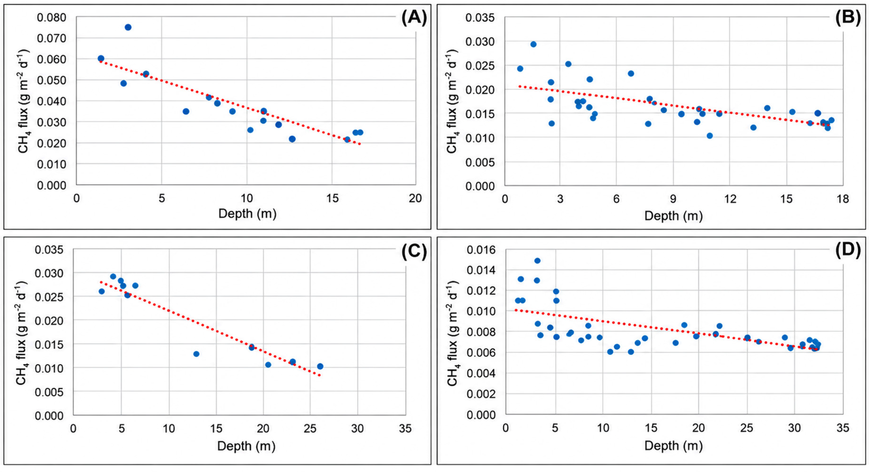
ΦCH₄ showed a strong inverse relationship with water depth during the 3rd survey (September 2023) at Congro Lake (r = −0.966) and Santiago Lake (r = −0.868), and during the 4th survey, made in December 2023 (respectively r = −0.636 and r = −0.659) (Figure 7). The lower diffusive flux at the surface in the areas where the depth is higher during the 3rd survey suggests the influence of stratification and/or more efficient surface water mixing. These mechanisms may cause more efficient oxidation as CH₄ slowly ascends by diffusion from the bottom of the lakes, allowing a more extensive microbial oxidation along the water column [87]. During winter, this inverse relationship is weaker, and there is lower methane production expected due to the lower temperature, suggesting that CH₄ is more able to avoid oxidation. Other studies have also shown the influence of water depth over methane emissions in surface water bodies [6,88].

Besides water depth, ΦCH₄ may also be function of other intrinsic drivers, such as the surface area, hydrologic regime, lake level variation, trophic state, and extrinsic factors, such as the climate (temperature and precipitation) and the watershed topography [12,78,89,90,91,92]. Data from the Congro and Santiago lakes does not depict any relationship between ΦCH₄ and the EC values, thus it does not suggest that water salinity controls flux as observed in other studies [93]. Both the studied lakes are currently eutrophic, as indicated by the Carlson TSITP index, which consistently exceeded 50 from 2017 to 2022 [94], and this trophic state may also enhance methane emissions, consistent with previous studies that have linked eutrophication to increased CH₄ fluxes due to higher organic matter input and subsequent microbial activity [7,92,95].

5.4. Overall CO₂ and CH₄ Emissions

The overall ΦCO₂ flux was estimated applying sGs method as equal to 0.18 t d⁻¹ and 0.11 t d⁻¹, respectively for the 1st and 2nd surveys made at Congro Lake, and to 1.88 t d⁻¹ to 0.22 t d⁻¹ at Santiago Lake (

Table 3. Overall ΦCO₂ estimated in the studied lakes through sGs and GSA methods according to the sampling survey (the integrated flux over the area of the water bodies is estimated using values from sGs as reference).

Lake	Survey	Working Area (km2)	ΦCO2 (t d−1) (sGs)	ΦCO2 (t d−1) (GSA)	ΦCO2 (t km−2 d−1)
Congro	1	0.038	0.18	0.24	4.74
	2	0.040	0.11	0.12	2.75
Santiago	1	0.253	1.88	1.83	7.43
	2	0.231	0.22	0.32	0.95

). Integrating the values over the area of the water bodies, fluxes are also higher at Santiago (7.43 t km⁻² d⁻¹ and 0.95 t km⁻² d⁻¹ for the 1st and 2nd surveys, respectively) relative to Congro Lake during the 1st survey (4.74 t km⁻² d⁻¹ and 2.75 t km⁻² d⁻¹), but instead along the 2nd survey flux per km² is higher at Congro Lake. This suggests that during periods of stratification, CO₂ emissions are less influenced by the total surface area of the lake and more dependent on localized degassing from shallower regions, particularly near the lake margins. Stratification limits CO₂ release by trapping gas within the hypolimnion, reducing overall emissions despite a larger surface area available for diffusion. In contrast, during mixing periods, CO₂ accumulated in deeper layers is released more uniformly across the lake surface (Figure 4A–D).

GSA values are very similar to the ones estimated by sGs in both lakes, in the range of 0.24 t d⁻¹ (6.32 t km⁻² d⁻¹) and 0.12 t d⁻¹ (3.00 t km⁻² d⁻¹) and between 1.83 t d⁻¹ (7.35 t km⁻² d⁻¹) to 0.32 t d⁻¹ (1.38 t km⁻² d⁻¹), respectively, for Congro and Santiago lakes along the 1st and 2nd surveys (Table 3). These values are in the lower range relative to the GSA ΦCO₂ dataset compiled by [37], which comprises a representative collection of 45 lake water bodies in the Azores, with estimates varying between 0.43 and 508.33 t km⁻² d⁻¹ (mean = 18.05 ± 71.7 t km⁻² d⁻¹; median = 4.61 t km⁻² d⁻¹; n = 68). Nevertheless, excluding from this dataset the two lakes that are outliers due to their very high fluxes (Furna do Enxofre and Furnas lakes) resulting from the influence of a deep-seated CO₂ source, values estimated for Congro and Santiago lakes during full mixing conditions are close to the mean (5.70 ± 6.04 t km⁻² d⁻¹) and median (4.51 t km⁻² d⁻¹; n = 65).

To obtain a preliminary estimate of whole-lake diffusive ΦCH₄ emissions in both lakes, the surface area of the water bodies was divided into two sections according to depth. The areas corresponding to depths lower and higher than 5 m were calculated, and the mean ΦCH₄ values measured within each depth interval were assigned to the respective subareas. Based on this simplified depth based extrapolation, the whole-lake diffuse ΦCH₄ emissions along the 4th survey were estimated at 0.635 kg d⁻¹ and 1.885 kg d⁻¹, respectively for the Congro and Santiago lakes, which are much lower than the corresponding ΦCO₂ emissions under the same hydrological conditions (e.g., stratification of the water column), corresponding to 16.71 kg km⁻² d⁻¹ and 8.16 kg km⁻² d⁻¹. Despite the smaller number of SFC measurements, the corresponding preliminary estimates for the 3rd survey were 1.30 kg d⁻¹ (34.21 kg km⁻² d⁻¹) and 4.38 kg d⁻¹ (17.31 kg km⁻² d⁻¹), respectively. These preliminary whole-lake estimates fall within the lower range of methane fluxes compiled by [23] for lakes with areas between 0.01 and 0.1 km² (Q1 = 12.2 kg km⁻² d⁻¹; Q3 = 94.4 kg km⁻² d⁻¹; median = 40.7 kg km⁻² d⁻¹) and between 0.1 and 1 km² (Q1 = 6.9 kg km⁻² d⁻¹; Q3 = 57.0 kg km⁻² d⁻¹; median = 20.8 kg km⁻² d⁻¹), being closer to the median value along the 3rd survey.

Despite the low ΦCH₄ relative to ΦCO₂ values, the former is a GHG with a global warming potential over a 100-year time span 27 times higher than the latter [96], amplifying its climate impact. In this context, the total GHG emissions from the studied lakes to the atmosphere is estimated as equal to 0.145 t CO_2-eq d⁻¹ and 0.338 t CO_2-eq d⁻¹, respectively, for Congro and Santiago lakes in stratified conditions, and between 0.197 t CO_2-eq d⁻¹and 1.91 t CO_2-eq d⁻¹ during full mixing conditions along the water column, being governed mostly by CO₂. In terms of CO_2-eq the ΦCO₂ are 2 to 3 times higher than ΦCH₄ when the lakes are stratified in summer period, and 10 to 35 times higher during full mixing conditions. This dominance is also expected even in lakes located in active volcanic systems, as, besides being a minor component relative to CO₂ in geothermal and volcanic emissions worldwide [29], the global methane volcanic emission from volcanoes was estimated as being lower than 1 Tg yr⁻¹, corresponding to a mean value 3 to 4 measures of magnitude lower than carbon dioxide [97,98].

6. Conclusions

The ΦCO₂ and ΦCH₄ from lakes into the atmosphere have been studied worldwide due to the perception of these water bodies as emitters of greenhouse gases. The present study addresses carbon dioxide and methane emissions from two maar crater lakes and identifies seasonal associations between gas fluxes and microbial community composition. While the observed associations are consistent with the current understanding of microbial carbon cycling, the present data do not provide sufficient evidence to establish direct causal relationships between specific microbial taxa and whole-lake greenhouse gas emissions. Nevertheless, the results suggest seasonal differences in microbial community composition, reflected by shifts in the relative abundance of specific microbial taxa, particularly during winter. However, longer-term monitoring and additional sampling campaigns will be required to confirm the temporal consistency of these patterns and further evaluate their potential association with greenhouse gas emissions.

Bacterial families usually associated with CO₂ production, including those involved in heterotrophic respiration, fermentation, and syntrophic metabolism, were identified in both lakes, the most abundant taxa being Clostridiaceae, Enterobacteriaceae, Holophagaceae, Smithellaceae and Methylomonadaceae. During winter the most abundant taxa, like Clostridiaceae and Enterobacteriaceae, depict higher abundances, suggesting intensified fermentation, reflected in the higher total ΦCO₂ estimated by sGs during colder conditions at the Congro (0.18 t d⁻¹) and Santiago (0.22 t d⁻¹) lakes, that corresponded to a mean value equal, respectively, to 6.4 g m⁻² d⁻¹ and 7.2 g m⁻² d⁻¹. Nevertheless, during summer Methylomonadaceae, a bacterial family responsible for methane oxidation, and subsequent CO₂ production, shown a higher abundance in both lakes, but particularly in Congro.

Methanogenic archaea, particularly members of the Methanobacteriaceae and Methanosarcinaceae, were more abundant during summer and may be associated with the observed seasonal increase in methane emissions. At Congro Lake, Methanosarcinaceae showed a slight increase in relative abundance during summer; whereas, at Santiago Lake, Syntrophaceae and unclassified Syntrophales were also more abundant under warmer conditions. During this period, mean ΦCH₄ is equal to 0.036 g m⁻² d⁻¹ and 0.020 g m⁻² d⁻¹, respectively, at the Congro and Santiago Lakes, approximately twice the values observed during the colder season. While these observations are consistent with the known ecological role of methanogenic microorganisms, the present data indicate an association rather than a direct causal relationship between microbial community composition and whole-lake methane emissions.

Moreover, the empirical flux data is controlled by the monomictic behavior of both water bodies. When stratification conditions prevail, CO₂ emissions are less influenced by the total surface area of the lake and more dependent on localized degassing from shallower regions, particularly near the lake margins. Stratification limits CO₂ release by trapping gas within the hypolimnion, reducing overall emissions despite a larger surface area available for diffusion.

Considering CO_2-eq, ΦCO₂ is 2 to 3 times higher than ΦCH₄ when the lakes are stratified in summer period, and 10 to 35 times higher during full mixing conditions. This is consistent with results obtained in studies made worldwide, and even in active volcanic regions methane is just a minor component compared to CO₂ in geothermal and volcanic emissions.

The results of this study highlight the need for further research, to address some remaining knowledge gaps and overcome limitations of the present study. Future work should focus on quantifying the uncertainties associated with the floating chamber methodology and improving the representativeness of ΦCH₄ measurements through additional surveys during the summer period and a denser spatial sampling network, which was not previously possible due to logistical constraints. These improvements would also allow the preliminary whole-lake methane emission estimates presented in this study to be further refined. Extending the monitoring period would also help to better constrain seasonal variability. Another important aspect requiring further investigation is the determination of the methane emissions associated with the ebullition process, which was not addressed in the present study and represents an important source of uncertainty in the whole-lake methane emissions estimates.

Through the integrated research of dissolved gases and water chemistry, the present study contributes to a better understanding of volcanic gas emissions from lake water bodies in volcanic settings. This is especially relevant in the case of methane, for which published datasets remain considerably scarcer than those available for CO₂. As both CH₄ and CO₂ are greenhouse gases, these findings also provide valuable information for improving greenhouse gas budgets and supporting future climate change studies.

References

1. Cole, J.J.; Caraco, N.F.; Kling, G.W.; Kratz, T.K. Carbon dioxide supersaturation in the surface waters of lakes. Science 1994, 265, 1568–1570. [Google Scholar] [CrossRef] [PubMed]
2. Tranvik, L.J.; Downing, J.A.; Cotner, J.B.; Loiselle, S.A.; Striegl, R.G.; Ballatore, T.J.; Dilon, P.; Finlay, K.; Fortino, K.; Knoll, L.B.; et al. Lakes and reservoirs as regulators of carbon cycling and climate. Limnol. Oceanogr. 2009, 54, 2298–2314. [Google Scholar] [CrossRef]
3. Raymond, P.A.; Hartmann, J.; Lauerwald, R.; Sobek, S.; McDonald, C.; Butman, D.; Striegl, R.; Mayorga, E.; Humborg, C.; Kortelainen, P.; et al. Global carbon dioxide emissions from inland waters. Global carbon dioxide emissions from inland waters. Nature 2013, 503, 355–359. [Google Scholar] [CrossRef] [PubMed]
4. Holgerson, M.; Raymond, P. Large contribution to inland water CO2 and CH4 emissions from very small ponds. Nat. Geosci. 2016, 9, 222–226. [Google Scholar] [CrossRef]
5. DelSontro, T.; Beaulieu, J.J.; Downing, J.A. Greenhouse gas emissions from lakes and impoundments: Upscaling in the face of global change. Limnol. Oceanogr. Lett. 2018, 3, 64–75. [Google Scholar] [CrossRef]
6. Li, M.; Peng, C.; Zhu, Q.; Zhou, X.; Yang, G.; Song, X.; Zhang, K. The significant contribution of lake depth in regulating global lake diffusive methane emissions. Water Res. 2020, 172, 115465. [Google Scholar] [CrossRef] [PubMed]
7. Beaulieu, J.J.; DelSontro, T.; Downing, J.A. Eutrophication will increase methane emissions from lakes and impoundments during the 21st century. Nat. Commun. 2019, 10, 1375. [Google Scholar] [CrossRef] [PubMed]
8. Pellegrinetti, T.A.; Cotta, S.R.; Feitosa, Y.B.; Melo, P.L.A.; Bieluczyk, W.; Silva, A.M.M.; Mendes, L.W.; Sarmento, H.; Camargo, P.B.; Tsai, S.M.; et al. The role of microbial communities in biogeochemical cycles and greenhouse gas emissions within tropical soda lakes. Sci. Total Environ. 2020, 947, 174646. [Google Scholar] [CrossRef] [PubMed]
9. Ehhalt, D.H. The atmospheric cycle of methane. Tellus 1974, 26, 58–70. [Google Scholar] [CrossRef]
10. Smith, L.K.; Lewis, W.M. Seasonality of methane emissions from five lakes and associated wetlands of the colorado rockies. Glob. Biogeochem. Cycles 1992, 6, 323–338. [Google Scholar] [CrossRef]
11. St. Louis, V.L.; Kelly, C.A.; Duchemin, É.; Rudd, J.W.; Rosenberg, D.M. Reservoir surfaces as sources of greenhouse gases to the atmosphere: A global estimate. BioScience 2000, 50, 766–775. [Google Scholar] [CrossRef]
12. Bastviken, D.; Cole, J.; Pace, M.; Tranvik, L. Methane emissions from lakes: Dependence of lake characteristics, two regional assessments, and a global estimate. Glob. Biogeochem. Cycles 2004, 18, GB4009. [Google Scholar] [CrossRef]
13. Bastviken, D.; Tranvik, L.J.; Downing, J.A.; Crill, P.M.; Enrich-Prast, A. Freshwater methane emissions offset the continental carbon sink. Science 2011, 331, 50. [Google Scholar] [CrossRef] [PubMed]
14. Cao, M.; Gregson, K.; Marshall, S. Global methane emission from wetlands and its sensitivity to climate change. Atmos. Environ. 1998, 32, 3293–3299. [Google Scholar] [CrossRef]
15. Walter, B.; Heimann, M.; Matthews, E. Modeling modern methane emissions from natural wetlands 1. Model description and result. J. Geophys. Res. 2001, 106, 34189–34206. [Google Scholar] [CrossRef]
16. Zhu, Q.; Peng, C.; Chen, H.; Fang, X.; Liu, J.; Jiang, H.; Yang, Y.; Yang, G. Estimating global natural wetland methane emissions using process modelling: Spatio-temporal patterns and contributions to atmospheric methane fluctuations. Glob. Ecol. Biogeogr. 2015, 24, 959–972. [Google Scholar] [CrossRef]
17. Rocher-Ros, G.; Stanley, E.H.; Loken, L.C.; Casson, N.J.; Raymond, P.A.; Liu, S.; Amatulli, G.; Sponseller, R.A. Global methane emissions from rivers and streams. Nature 2023, 621, 530–535. [Google Scholar] [CrossRef] [PubMed]
18. Saunois, M.; Bousquet, P.; Poulter, B.; Peregon, A.; Ciais, P.; Canadell, J.G.; Dlugokencky, E.J.; Etiope, G.; Bastviken, D.; Houweling, S.; et al. The global methane budget 2000–2012. Earth Syst. Sci. Data 2016, 8, 697–751. [Google Scholar] [CrossRef]
19. Saunois, M.; Martinez, A.; Poulter, B.; Zhang, Z.; Raymond, P.A.; Regnier, P.; Canadell, J.G.; Jackson, R.B.; Patra, P.K.; Bousquet, P.; et al. Global Methane Budget 2000–2020. Earth Syst. Sci. Data 2025, 17, 1873–1958. [Google Scholar] [CrossRef]
20. Saunois, M.; Stavert, A.R.; Poulter, B.; Bousquet, P.; Canadell, J.G.; Jackson, R.B.; Raymond, P.A.; Dlugokencky, E.J.; Houweling, S.; Patra, P.K.; et al. The global methane budget 2000–2017. Earth Syst. Sci. Data 2020, 12, 1561–1623. [Google Scholar] [CrossRef]
21. Johnson, M.S.; Matthews, E.; Du, J.; Genovese, V.; Bastviken, D. Methane emission from global lakes: New spatiotemporal data and observation-driven modeling of methane dynamics indicates lower emissions. J. Geophys. Res. Biogeosci. 2022, 127, e2022JG006793. [Google Scholar] [CrossRef] [PubMed]
22. Zhuang, Q.; Guo, M.; Melack, J.M.; Lan, X.; Tan, Z.; Oh, Y.; Leung, L.R. Current and future global lake methane emissions: A process-based modeling analysis. J. Geophys. Res. Biogeosci. 2023, 128, e2022JG007137. [Google Scholar] [CrossRef]
23. Rosentreter, J.A.; Borges, A.V.; Deemer, B.R.; Holgerson, M.A.; Liu, S.; Song, C.; Melack, J.; Raymond, P.A.; Duarte, C.M.; Allen, G.H.; et al. Half of global methane emissions come from highly variable aquatic ecosystem sources. Nat. Geosci. 2021, 14, 225–230. [Google Scholar] [CrossRef]
24. DROTRH-INAG. Plano Regional Da Água. Relatório Técnico; Direção Regional do Ordenamento do Território e do Ordenamento do Território: Ponta Delgada, Portugal, 2001; p. 575. (In Portuguese) [Google Scholar]
25. Porteiro, J. Lagoas dos Açores: Elementos de Suporte ao Planeamento Integrado. PhD Thesis, Universidade dos Açores, Ponta Delgada, Portugal, 2000. (In Portuguese) [Google Scholar]
26. AHA-DRA. Plano de Gestão da Região Hidrográfica dos Açores—RH9; Versão para consulta pública; AHA-DRA: Ponta Delgada, Portugal, 2015. (In Portuguese) [Google Scholar]
27. Cruz, J.V.; Antunes, P.; França, Z.; Nunes, J.C.; Amaral, C. Volcanic lakes from the Azores archipelago (Portugal): Geological setting and geochemical characterization. J. Volcanol. Geotherm. Res. 2006, 156, 135–157. [Google Scholar] [CrossRef]
28. Pérez, N.M.; Hernández, P.A.; Padilla, G.; Nolasco, D.; Barrancos, J.; Melián, G.; Padrón, E.; Dionis, S.; Calvo, D.; Rodríguez, F.; et al. Global CO2 emission from volcanic lakes. Geology 2011, 39, 235–238. [Google Scholar] [CrossRef]
29. Etiope, G.; Ciotoli, G.; Schwietzke, S.; Schoell, M. Gridded maps of geological methane emissions and their isotopic signature. Earth Syst. Sci. Data 2019, 11, 1–22. [Google Scholar] [CrossRef]
30. Andrade, C.; Viveiros, F.; Cruz, J.V.; Coutinho, R.; Silva, C. Estimation of the CO2 flux from Furnas volcanic lake (São Miguel, Azores). J. Volcanol. Geotherm. Res. 2016, 315, 51–64. [Google Scholar] [CrossRef]
31. Andrade, C.; Viveiros, F.; Cruz, J.V.; Branco, R.; Moreno, L.; Silva, C.; Coutinho, R.; Pacheco, J. Diffuse CO2 flux emission in two maar crater lakes from São Miguel (Azores, Portugal). J. Volcanol. Geotherm. Res. 2019, 369, 188–202. [Google Scholar] [CrossRef]
32. Andrade, C.; Cruz, J.V.; Viveiros, F.; Coutinho, R. CO2 flux from volcanic lakes in the western group of the Azores archipelago (Portugal). Water 2019, 11, 599. [Google Scholar] [CrossRef]
33. Andrade, C.; Cruz, J.V.; Viveiros, F.; Branco, R.; Coutinho, R. CO2 degassing from Pico Island (Azores, Portugal) volcanic lakes. Limnologica 2019, 76, 72–81. [Google Scholar] [CrossRef]
34. Andrade, C.; Viveiros, F.; Cruz, J.V.; Coutinho, R.; Branco, R. CO2 flux from two lakes in volcanic caves in the Azores (Portugal). Appl. Geochem. 2019, 102, 218–228. [Google Scholar] [CrossRef]
35. Andrade, C.; Cruz, J.V.; Viveiros, F.; Coutinho, R. CO2 emissions from Fogo intracaldeira volcanic lakes (São Miguel Island, Azores): A tool for volcanic monitoring. J. Volcanol. Geotherm. Res. 2020, 400, 106915. [Google Scholar] [CrossRef]
36. Andrade, C.; Cruz, J.V.; Viveiros, F.; Coutinho, R. Diffuse CO2 emissions from Sete Cidades volcanic lake (São Miguel Island, Azores): Influence of eutrophication processes. Environ. Pollut. 2020, 268, 115624. [Google Scholar] [PubMed]
37. Andrade, C.; Viveiros, F.; Cruz, J.V.; Coutinho, R. Global carbon dioxide output of volcanic lakes in the Azores archipelago, Portugal. J. Geochem. Explor. 2021, 229, 106835. [Google Scholar] [CrossRef]
38. Tassi, F.; Cabassi, J.; Andrade, C.; Callieri, C.; Silva, C.; Viveiros, F.; Corno, G.; Vaselli, O.; Selmo, E.; Gallorini, A.; et al. Mechanisms regulating CO2 and CH4 dynamics in the Azorean volcanic lakes (São Miguel Island, Portugal). J. Limnol. 2018, 77, 483–504. [Google Scholar] [CrossRef]
39. Andrade, C.; Cruz, J.V.; Ferreira, L.; Viveiros, F.; Toubarro, D.; Tassi, F.; Pimentel, A.; Braga, D.; Cordeiro, A.; Raposeiro, P. Diffuse CO2 and CH4 emissions of two Volcanic lakes on Pico Island (Azores). J. Volcanol. Geotherm. Res. 2025, 467, 108424. [Google Scholar] [CrossRef]
40. Cruz, J.V.; Andrade, C.; Toubarro, D.; Ferreira, L.; Pimentel, A.; Viveiros, F.; Tassi, F.; Cordeiro, A.; Braga, D.; Raposeiro, P. C-based gas (CH4 and CO2) fluxes from eutrophicated Volcanic shallow lakes in Corvo Island (Azores, Portugal). Appl. Geochem. 2025, 191, 106529. [Google Scholar] [CrossRef]
41. Ferreira, T.; Gomes, A.; Gaspar, J.L.; Guest, J. Distribution and significance of basaltic eruptive centres: São Miguel, Azores. In Volcanic Geology of São Miguel Island (Azores Archipelago); Gaspar, J.L., Guest, J.E., Duncan, A.M., Barriga, F.J.A.S., Chester, D.K., Eds.; Geological Society of London: London, UK, 2015; Volume 44, pp. 135–146. [Google Scholar]
42. Moore, R.B. Geology of Three Late Quaternary Stratovolcanoes on São Miguel, Azores; US Geological Survey Bulletin: Washington, DC, USA, 1991; p. 1900.
43. Booth, B.; Croasdale, R.; Walker, G. A quantitative study of five thousand years of volcanism on São Miguel Azores. Phil. Trans. R. Soc. Lond. 1978, 288, 271–319. [Google Scholar] [CrossRef]
44. Moore, R.; Rubin, M. Radiocarbon dates for lava flows and pyroclastic deposits on São Miguel, Azores. Radiocarbon 1991, 33, 151–164. [Google Scholar] [CrossRef]
45. Queiroz, G.; Pacheco, J.M.; Gaspar, J.L.; Aspinall, W.P.; Guest, J.E.; Ferreira, T. The last 5000 years of activity at Sete Cidades volcano (São Miguel Island, Azores): Implications for hazard assessment. J. Volcanol. Geotherm. Res. 2008, 178, 562–573. [Google Scholar] [CrossRef]
46. Queiroz, G.; Gaspar, J.L.; Guest, J.E.; Gomes, A.; Almeida, M.H. Eruptive history and evolution of Sete Cidades Volcano, São Miguel Island, Azores. In Volcanic Geology of São Miguel Island (Azores Archipelago); Gaspar, J.L., Guest, J.E., Duncan, A.M., Barriga, F.J.A.S., Chester, D.K., Eds.; Geological Society of London: London, UK, 2015; Volume 44, pp. 87–104. [Google Scholar]
47. Queiroz, G. Vulcão das Sete Cidades (S. Miguel, Açores)—História Eruptiva e Avaliação do Hazard. Ph.D. Thesis, Universidade dos Açores, Ponta Delgada, Portugal, 1997; p. 266, (In Portuguese with English abstract). [Google Scholar]
48. Conte, E.; Widomchiodini, E.; Kuentz, D.; França, Z. 14C and U-series disequilibria age constraints from recent eruptions at Sete Cidades volcano, Azores. J. Volcanol. Geotherm. Res. 2019, 373, 167–178. [Google Scholar] [CrossRef]
49. APHA-AWWA-WPCF. Standard Methods for the Examination of Water and Methods for the Examination of Water and Wastewater; American Public Health Association: Washington, DC, USA, 1985. [Google Scholar]
50. IAEA. Sampling Procedures for Isotope Hydrology; Water Resources Programe; IAEA: Vienna, Austria, 2017; 8p. [Google Scholar]
51. Chiodini, G.; Cioni, R.; Guidi, M.; Raco, B.; Marini, L. Soil CO2 flux measurements in volcanic and geothermal areas. App. Geochem. 1998, 13, 543–552. [Google Scholar] [CrossRef]
52. Mazot, A.; Bernard, A. CO2 Degassing from Volcanic. In Volcanic Lakes, Advances in Volcanology; Rouwet, D., Christenson, B., Tassi, F., Vandemeulebrouck, J., Eds.; Springer: Heidelberg, Germany, 2015; pp. 341–354. [Google Scholar]
53. Gålfalk, M.; Bastviken, D.; Fredriksson, S.; Arneborg, L. Determination of the piston velocity for water–air interfaces using flux chambers, acoustic Doppler velocimetry, and IR imaging of the water surface. J. Geophys. Res. Biogeosci. 2013, 118, 770–782. [Google Scholar] [CrossRef]
54. Kremer, J.N.; Nixon, S.W.; Buckley, B.; Roques, P. Technical note: Conditions for using the floating chamber method to estimate air–water gas exchange. Estuaries 2003, 26, 985–990. [Google Scholar] [CrossRef]
55. System, W. Carbon Dioxide Flux Meter Handbook; West Systems srl: Pontedera, Italy, 2014; 123p. [Google Scholar]
56. Guseva, S.; Aurela, M.; Cortés, A.; Kivi, R.; Lotsari, E.; MacIntyre, S.; Mammarella, I.; Ojala, A.; Stepanenko, V.; Uotila, P.; et al. Variable physical drivers of near-surface turbulence in a regulated river. Water Resour. Res. 2021, 57, e2020WR027939. [Google Scholar] [CrossRef]
57. Cardellini, C.; Chiodini, G.; Frondini, F. Application of stochastic simulation to CO2 flux from soil. Mapping and quantification of gas release. J. Geophys. Res. 2003, 108, 2425. [Google Scholar] [CrossRef]
58. Sinclair, A.J. Selection of threshold values in geochemical data using probability graphs. J. Geochem. Explor. 1994, 3, 129–149. [Google Scholar]
59. Sun, Y.; Guo, Z.; Liu, J.; Du, J. CO2 diffuse emission from maar lake: An example in Changbai volcanic field, NE China. J. Volcanol. Geotherm. Res. 2017, 349, 146–162. [Google Scholar]
60. David, M. Geostatistical Ore Reserve Estimation; Elsevier: New York, NY, USA, 1977; 364p. [Google Scholar]
61. Deutsch, C.V.; Journel, A.G. GSLIB: Geostatistical Software Library and User Guide, 2nd ed.; Oxford University: Oxford, UK, 1998; 363p. [Google Scholar]
62. Cardellini, C.; Chiodini, G.; Frondini, F.; Avino, R.; Bagnato, E.; Caliro, S.; Lelli, M.; Rosiello, A. Monitoring diffuse volcanic degassing during volcanic unrests: The case of Campi Flegrei (Italy). Sci. Rep. 2017, 7, 6757. [Google Scholar] [CrossRef] [PubMed]
63. Cole, J.J.; Bade, D.L.; Bastviken, D.; Pace, M.L.; Van de Bogert, M. Multiple approaches to estimating air-water gas exchange in small lakes. Limnol. Oceanogr. Methods 2010, 8, 285–293. [Google Scholar] [CrossRef]
64. Livingston, G.P.; Hutchinson, G.L. Enclosure-based measurement of trace gas exchange: Applications and sources of error. In Biogenic Trace Gases: Measuring Emissions from Soil and Water; Matson, P., Harriss, R., Eds.; Blackwell Science: Oxford, UK, 1995; pp. 14–51. [Google Scholar]
65. Mannich, M.; Fernandes, C.V.; Bleninger, T.B. Uncertainty analysis of gas flux measurements at air–water interface using floating chambers. Ecohydrol. Hydrobiol. 2019, 19, 475–486. [Google Scholar] [CrossRef]
66. Kutzbach, L.; Schneider, J.; Sachs, T.; Giebels, M.; Nykanen, H.; Shurpali, N.J.; Martikainen, P.J.; Alm, J.; Wilmking, M. CO2 flux determination by closed-chamber methods can be seriously biased by inappropriate application of linear regression. Biogeosciences 2007, 4, 1005–1025. [Google Scholar] [CrossRef]
67. Ghioldi, G.C. An Appraisal on Methane Emissions From Wetlands Based on Direct Estimates and Theroretical Computations: The Case of Lake Porta Wetland, Northern Tuscany (Italy). Master’s Thesis, Università degli Studi di Firenze, Florence, Italy, 2021; 92p. [Google Scholar]
68. Liss, P.S.; Slater, P.G. Flux of gases across the Air-Sea Interface. Nature 1974, 247, 182–184. [Google Scholar] [CrossRef]
69. Wanninnkhof, R. Relationship between wind speed and gas exchange over the ocean revisited. Limnol. Oceanogr. Methods 2014, 12, 351–362. [Google Scholar] [CrossRef]
70. Crusius, J.; Wanninnkhof, R. Gas transfer velocities measured at low wind speed over a lake. Limnol. Oceanogr. 2003, 48, 1010–1017. [Google Scholar] [CrossRef]
71. Andrade, C.; Cruz, J.V.; Viveiros, F.; Moreno, L.; Ferreira, L.; Coutinho, R. Hydrogeochemical evolution and characterization study in volcanic lakes of the Azores archipelago (Portugal). App. Geochem. 2024, 164, 105933. [Google Scholar] [CrossRef]
72. Cartigny, P.; Harris, J.W.; Javoy, M. Diamond genesis, mantle fractionations and mantle nitrogen content: A study of δ13C–N concentrations in diamonds. Earth Planet Sci. Lett. 2001, 185, 85–98. [Google Scholar] [CrossRef]
73. Clark, I. Groundwater Geochemistry and Isotopes; CRC Press, Taylor & Francis Group: Boca Raton, FL, USA, 2015; 456p. [Google Scholar]
74. Parkhurst, D.L.; Appelo, C.A.J. User’s Guide to Phreeqc (Version 2)—A Computer Program for Speciation, Batch-Reaction, One-Dimensional Transport, and Inverse Geochemical Calculations; Water-Resources Investigations Report 99-4259; USGS: Denver, CO, USA, 1999. [Google Scholar]
75. Hofmann, H. Spatiotemporal distribution patterns of dissolved methane in lakes: How accurate are the current estimations of the diffusive flux path? Geophys. Res. Lett. 2013, 40, 2779–2784. [Google Scholar] [CrossRef]
76. Eugster, W.; DelSontro, T.; Shaver, G.R.; Kling, G.W. Interannual, summer, and diel variability of CH4 and CO2 effluxes from Toolik Lake, Alaska, during the ice-free periods 2010–2015. Environ. Sci. Process. Impacts 2020, 22, 2181–2198. [Google Scholar] [PubMed]
77. Xiao, Q.; Zhang, M.; Hu, Z.; Gao, Y.; Hu, C.; Liu, C.; Liu, S.; Zhang, Z.; Zhao, J.; Xiao, W.; et al. Spatial variations of methane emission in a large shallow eutrophic lake in subtropical climate. J. Geophys. Res. Biogeosci. 2017, 122, 1597–1614. [Google Scholar] [CrossRef]
78. Fuchs, A.; Lyautey, E.; Montuelle, B.; Casper, P. Effects of increasing temperatures on methane concentrations and methanogenesis during experimental incubation of sediments from oligotrophic and mesotrophic lakes. J. Geophys. Res. Biogeosci. 2016, 121, 1394–1406. [Google Scholar] [CrossRef]
79. Duc, N.T.; Crill, P.; Bastviken, D. Implications of temperature and sediment characteristics on methane formation and oxidation in lake sediements. Biogeochemistry 2010, 100, 185–196. [Google Scholar] [CrossRef]
80. Xun, F.; Fenga, M.; Ma, S.; Chen, H.; Zhanga, W.; Mao, Z.; Zhou, Y.; Xiao, Q.; Wu, Q.L.; Xing, P. Methane ebullition fluxes and temperature sensitivity in a shallow lake. Sci. Total Environ. 2024, 912, 169589. [Google Scholar] [CrossRef] [PubMed]
81. Jansen, J.; Woolway, R.L.; Kraemer, B.M.; Albergel, C.; Bastviken, D.; Weyhenmeyer, G.A.; Marcé, R.; Sharma, S.; Sebastian Sobek, S.; Tranvik, L.J.; et al. Global increase in methane production under future warming of lake bottom waters. Glob. Change Biol. 2022, 28, 5427–5440. [Google Scholar] [CrossRef]
82. Schroll, M.; Liu, L.; Einzmann, T.; Keppler, F.; Grossart, H.-G. Methane accumulation and its potential precursor compounds in the oxic surface water layer of two contrasting stratified lakes. Sci. Total Environ. 2023, 903, 166205. [Google Scholar] [CrossRef] [PubMed]
83. Grossart, H.-P.; Frindte, K.; Dziallas, C.; Eckert, W.; Tang, K.W. Microbial methane production in oxygenated water column of an oligotrophic lake. Proc. Natl. Acad. Sci. USA 2011, 108, 19657–19661. [Google Scholar] [CrossRef] [PubMed]
84. Ordóñez, C.; DelSontro, T.; Langenegger, T.; Donis, D.; Suarez, E.L.; McGinnis, D.F. Evaluation of the methane paradox in four adjacent pre-alpine lakes across a trophic gradient. Nat. Commun. 2023, 14, 2165. [Google Scholar] [CrossRef] [PubMed]
85. Encinas Fernández, J.; Peeters, F.; Hofmann, H. On the methane paradox: Transport from shallow water zones rather than pelagic production in lakes? J. Geophys. Res. Biogeosci. 2014, 119, 984–993. [Google Scholar]
86. Schindler, D.W.; Hecky, R.E.; Findlay, D.L.; Kasian, S.E.M. Euthrophication of lakes cannot be controlled by reducing nitrogen input: Results of a 37-year whole-ecossystem experiment. Environ. Sci. 2008, 115, 11254–11258. [Google Scholar] [CrossRef]
87. Venturi, S.; Tassi, F.; Cabassi, J.; Randazzo, A.; Lazzaroni, M.; Capecchiacci; Vietina, B.; Vaselli, O. Exploring methane drivers in wetlands: The cases of massaciuccoli and porta lakes (Northern Tuscany, Italy). Appl. Sci. 2021, 11, 12156. [Google Scholar] [CrossRef]
88. Zhong, J.; Yang, F.; Zhang, M.; Sun, C.; Wang, S.; Chen, Q.; Wanga, H.; Zhang, L. Water depth and productivity regulate methane (CH4) emissions from temperate cascade reservoirs in northern China. J. Hydrol. 2023, 626, 130170. [Google Scholar] [CrossRef]
89. Sanches, L.F.; Guenet, B.; Marinho, C.C.; Barros, N.; Esteves, F.A. Global regulation of methane emissions from natural lakes. Sci. Rep. 2019, 9, 255. [Google Scholar] [CrossRef] [PubMed]
90. Li, L.; Fuchs, A.; Ortega, S.R.; Xue, B.; Casper, P. Spatial methane pattern in a deep freshwater lake: Relation to water depth and topography. Sci. Total Environ. 2021, 764, 142829. [Google Scholar] [CrossRef] [PubMed]
91. Yuan, X.; Liu, Q.; Cui, B.; Xu, X.; Liang, L.; Sun, T.; Yan, S.; Wanga, X.; Li, C.; Li, S.; et al. Effect of water-level fluctuations on methane and carbon dioxide dynamics in a shallow lake of Northern China: Implications for wetland restoration. J. Hydrol. 2021, 597, 126169. [Google Scholar] [CrossRef]
92. Zhang, L.; Liao, Q.; Gao, R.; Luo, R.; Liua, C.; Zhonga, J.; Wanga, Z. Spatial variations in diffusive methane fluxes and the role of eutrophication in a subtropical shallow lake. Sci. Total Environ. 2021, 759, 143495. [Google Scholar] [CrossRef] [PubMed]
93. Liu, H.; Xiao, S.; Liu, W.; Wang, H.; Liu, Z.; Li, X.; Zhang, P.; Liu, J. Salinity decreases methane concentrations in Chinese lakes. Sci. Total Environ. 2024, 937, 173412. [Google Scholar] [CrossRef] [PubMed]
94. Malcata, A.; Pacheco, D.; Cymbron, R. Monitorização Da Qualidade Da Água Das Lagoas de São Miguel, Pico, Flores e Corvo. Comparação de Resultados Entre 2017 e 2020; SRAAC: Ponta Delgada, Portugal, 2022; 336p. (In Portuguese) [Google Scholar]
95. Zhang, J.; Cao, L.; Liu, Z.; Wan, L.; Cao, X.; Zhou, Y.; Songa, C. Relationship between eutrophication and greenhouse gases emission in shallow freshwater lakes. Sci. Total Environ. 2024, 925, 171610. [Google Scholar] [CrossRef] [PubMed]
96. Forster, P.; Storelvmo, T.; Armour, K.; Collins, W.; Dufresne, J.-L.; Frame, D.; Lunt, D.J.; Mauritsen, T.; Palmer, M.D.; Watanabe, M.; et al. The Earth’s Energy Budget, Climate Feedbacks, and Climate Sensitivity. In Climate Change 2021: The Physical Science Basis. Contribution of Working Group I to the Sixth Assessment Report of the Intergovernmental Panel on Climate Change; Masson-Delmotte, V., Zhai, P., Pirani, A., Connors, S.L., Péan, C., Berger, S., Caud, N., Chen, Y., Goldfarb, L., Gomis, M.I., et al., Eds.; Cambridge University Press: Cambridge, UK, 2021; pp. 923–1054. [Google Scholar] [CrossRef]
97. Etiope, G.; Lassey, K.R.; Klusman, R.W.; Boschi, E. Reappraisal of the fossil methane budget and related emission from geologic sources. Geophys. Res. Lett. 2008, 35, L09307. [Google Scholar] [CrossRef]
98. Mörner, N.-A.; Etiope, G. Carbon degassing from the lithosphere. Glob. Planet. Change 2002, 33, 185–203. [Google Scholar] [CrossRef]
Figure 1. Location of the studied lakes in São Miguel Island. (A) Azores archipelago location at about 1500 km West of Portugal mainland; (B) location of São Miguel Island (in red) in the eastern group of islands from the Azores; (C) location of the studied lakes in São Miguel Island; (D,E) Santiago and Congro lakes bathymetry, respectively (PS and PC, locations where samples were collected for water chemistry and microbial community characterization). UTM coordinates are used for plots (D,E) (UTM zone 26N).
Environments 13 00439 g001
Figure 2. Variation along the water column of the main physico-chemical parameters for the studied lakes, showing the effects of stratification during summer ((A) temperature, in °C; (B) pH, in pH units; (C) EC, electrical conductivity, in µS cm−1; (D) dissolved CO2, in mg L−1). Surveys 1 and 4 were made in winter of 2023 and surveys 2 and 3 during summer of 2023—shown in yellow (Congro Lake) and green (Santiago Lake).
Environments 13 00439 g002
Figure 3. Relationship between δ13C (‰) and the dissolved inorganic carbon (DIC) suggesting a single biogenic CO2-source. Additional data include mineral waters in São Miguel Island and lakes in the Azores archipelago from [71]. DIC concentrations (mol kg−1) were estimated by PHREEQC [74].
Environments 13 00439 g003
Figure 4. Results for the sequential Gaussian simulation represented by E-type CO2 flux (g m−2 d−1) maps for the Congro ((A) 1st measurement survey; (B) 2nd measurement survey) and Santiago lakes ((C) 1st measurement survey; (D) 2nd measurement survey). Surveys were made, respectively, during winter (1st measurement survey—March of 2023) and summer (2nd measurement survey—June of 2023).
Environments 13 00439 g004
Figure 5. Boxplot diagrams for the CH4 flux (g m−2 d−1) measurements ((A) 3rd survey—Congro Lake; (B) 3rd survey—Santiago Lake; (C) 4th survey—Congro Lake; (D) 4th survey—Santiago Lake). Surveys were made, respectively, during summer (3rd measurement survey—September of 2023) and summer (4th measurement survey—December of 2023).
Environments 13 00439 g005
Figure 6. CH4 flux (g m−2 d−1) measurements for the several surveys made in the studied lakes ((A) 3rd survey—Congro Lake; (B) 4th survey—Congro Lake; (C) 3rd survey—Santiago Lake; (D) 4th survey—Santiago Lake). The references on the plot are made with the number of each transect (left) and the number of the measurement point on the transect (right). Surveys were made respectively during summer (3rd measurement survey—September of 2023) and summer (4th measurement survey—December of 2023).
Environments 13 00439 g006
Figure 7. Relationship between CH4 flux (g m−2 d−1) measurements and the lake water depth (m) illustrated by a binary plot ((A) 3rd survey—Congro Lake; (B) 4th survey—Congro Lake; (C) 3rd survey—Santiago Lake; (D) 4th survey—Santiago Lake). Surveys were made during summer (3rd measurement survey—September of 2023) and summer (4th measurement survey—December of 2023).
Environments 13 00439 g007