Physical and Biogeochemical Drivers for Forecasting Red Tides in Southwest Florida: A Regionally Integrated Machine Learning Framework

Abstract

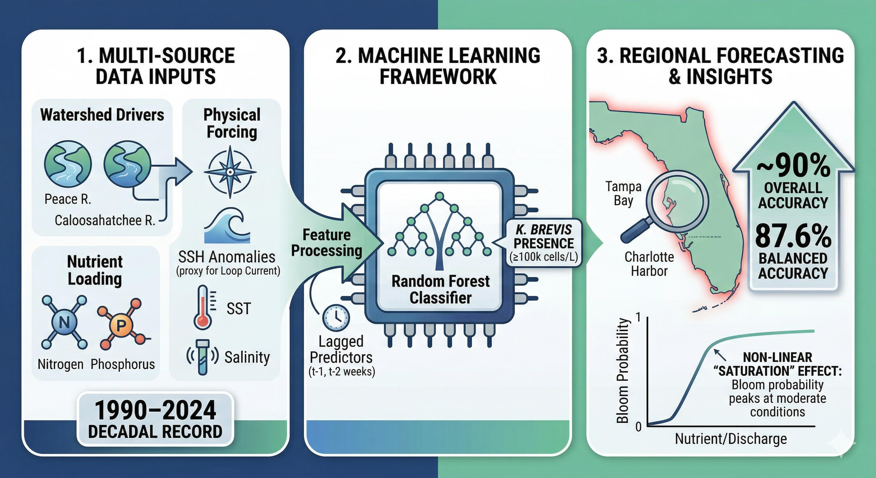
Harmful algal blooms (HABs) caused by Karenia brevis (K. brevis) present a persistent ecological and public health challenge across coastal Florida. Reliable bloom forecasting is critical for protecting public health, supporting coastal economies, and enabling timely management responses. This study develops a regionally integrated machine learning framework to predict weekly K. brevis bloom occurrence using environmental data from both the Peace and Caloosahatchee Rivers, combined with coastal bloom records from Southwest Florida and Tampa Bay to enhance the spatial and temporal continuity of the response record. A Random Forest classifier was trained on a multi-decadal dataset incorporating river discharge, nutrient concentrations (total nitrogen and total phosphorus), wind forcing, sea surface temperature, salinity, and sea surface height anomalies as a proxy for Loop Current variability. The model achieved strong predictive performance on a chronologically withheld test set, with an overall accuracy of ~90%, balanced accuracy of 87.6%, and ROC–AUC of 0.972, indicating strong discrimination between bloom and non-bloom conditions with high precision and recall for bloom events. Bloom timing and persistence were captured with strong agreement during ongoing bloom periods, while non-bloom conditions were identified with low false-positive rates. Feature-response analyses indicated that bloom probability increased most sharply under moderate discharge and nutrient conditions, with diminished sensitivity at higher extremes. Learning curve analysis demonstrated robust training performance and stable generalization, with validation accuracy plateauing near 84%, suggesting a data-limited ceiling on forecast skill. By aggregating nutrient inputs across multiple watersheds and integrating spatially aligned bloom observations, this study demonstrates the utility of multi-source machine learning frameworks for regional-scale HAB prediction. The results support the development of early warning tools and provide a reproducible foundation for evaluating how combined watershed loading and physical forcing are associated with K. brevis bloom occurrence in complex estuary systems with watershed and coastal coupling.

1. Introduction

Coastal water quality degradation driven by nutrient enrichment and harmful algal blooms (HABs) is an increasingly urgent environmental and public health concern worldwide [1,2]. Recent regional and global syntheses highlighting increasing frequency, intensity, and socio-economic impacts of HAB events, including risks to fisheries, aquaculture, tourism, public health and food security [3,4,5]. Along the West Florida Shelf, blooms of Karenia brevis (K. brevis), commonly referred to as red tide, are among the most persistent and damaging HABs, producing brevetoxins that cause respiratory illness, widespread fish kills, and substantial economic losses to coastal communities [6,7,8,9,10,11]. Although K. brevis blooms are a natural feature of the Gulf of Mexico, mounting evidence indicates that anthropogenic nutrient enrichment and altered hydrologic regimes may intensify bloom persistence and coastal impacts [7,12,13,14]. Recent long-term analyses indicate an increase in bloom duration and severity linked to climate variability, warming, and anthropogenic nitrogen loading [13,15]. Accordingly, accurate predictive tools are essential for early warning efforts in protecting public health, supporting coastal economies, and informing timely management responses.

Two major river systems, the Peace River and the Caloosahatchee River, exert strong influence on coastal water quality in southwest Florida by delivering freshwater, nutrients, and organic matter to nearshore waters. These rivers drain watersheds characterized by intensive agriculture, urban development, and managed flow control structures, creating highly variable discharge and nutrient loading conditions [16]. Previous studies have documented associations between riverine nutrient inputs, particularly total nitrogen (TN) and total phosphorus (TP), and K. brevis bloom development, though the relative importance of individual watersheds and nutrients remains debated [14,17]. Recent work [15] emphasizes the role of anthropogenic nitrogen inputs and watershed-scale loading in modulating bloom persistence. Importantly, nutrient delivery does not act in isolation but interacts with physical drivers such as wind forcing, shelf circulation, and Loop Current variability to regulate bloom transport, retention, and persistence [18,19,20,21].

Recent studies further highlight the increasing complexity of K. brevis bloom dynamics, including the combined influence of extreme weather events, biological interactions, and ecosystem-scale responses. For example, hurricane-driven nutrient pulses, river discharge, and wind-induced circulation have been shown to jointly regulate bloom initiation, transport, and intensity, with the timing of physical forcing relative to nutrient delivery playing a critical role in determining bloom outcomes [22,23]. More broadly, hurricane impacts can generate spatially heterogeneous phytoplankton responses, including rapid declines followed by rebounds in biomass and shifts in phytoplankton community structure across Gulf coast estuaries [23]. Beyond physical forcing, biological processes such as mixotrophy and microbial interactions can enhance bloom persistence under nutrient-limited conditions, support offshore expansion, and alter competitive dynamics within plankton communities [22,24,25,26]. Long-term satellite observations further indicate that red tide blooms have expanded in spatial extent, duration, and probability of occurrence across the West Florida Shelf over recent decades, suggesting broader environmental and climatic controls on bloom distribution [27]. Emerging data sources, including social sensing and alternative monitoring approaches, also provide additional insights into public perception and spatiotemporal patterns of bloom impacts [28]. Collectively, these findings underscore the need for integrated predictive frameworks that account for coupled physical, biogeochemical, ecological, and socio-environmental drivers.

Recent advances in machine learning have provided practical tools for modeling HABs in complex coastal systems [29,30,31,32,33,34], where nonlinear interactions and class imbalance limit the effectiveness of traditional statistical approaches [12]. Recent reviews [3,35] emphasize the growing role of integrating machine learning (ML), remote sensing, and multi-source observational systems for improved HAB monitoring and early warning. ML classifiers trained on physical and hydrologic drivers including Loop Current cycles, wind forcing, and river discharge have demonstrated a skill in distinguishing between large bloom and non-bloom conditions along the West Florida Shelf [36]. A similar framework [37] has integrated cumulative nutrient loading. While previous studies [36,37] have prioritized environmental drivers, recent research [16,34,38] suggests that incorporating autoregressive features (lagged bloom observations) can increase operational accuracy by capturing bloom persistence, though often at the expense of isolating the contribution of external environmental forcing.

However, distinct challenges remain regarding model sensitivity and spatial transferability. First, reliance on recent bloom history can bias predictions toward persistence, potentially obscuring the environmental drivers responsible for true bloom onset following non-bloom periods [16,34]. Second, models trained on restricted geographic domains may struggle to generalize about new regions. Specifically, it remains to be determined whether expanding the training domain of a localized Southwest Florida model by explicitly incorporating bloom records from adjacent coastal regimes such as Tampa Bay enhances predictive robustness and spatial generalization [34]. To address these needs, this study develops a regionally integrated machine learning framework to predict K. brevis bloom occurrence along the Southwest Florida coast. Building on existing ML approaches [36,37], the framework integrates watershed-scale nutrient concentrations (TN and TP) and discharge from both the Peace and Caloosahatchee Rivers, alongside atmospheric forcing, Loop Current variability, and local hydrographic conditions. Bloom observations from the Tampa Bay region are incorporated to expose the model to a broader range of bloom and non-bloom transitions and to evaluate whether such expansion improves predictive robustness for the Southwest Florida domain. Lagged bloom predictors are included to represent short-term biological persistence rather than to resolve bloom initiation mechanisms [16], while the relative predictive influence of cumulative nutrient concentrations and physical forcing is quantified under these conditions. By synthesizing these data sources, this study provides a reproducible framework for evaluating environmental conditions associated with regional K. brevis bloom occurrence.

2. Methods

2.1. Study Area and Bloom Observations

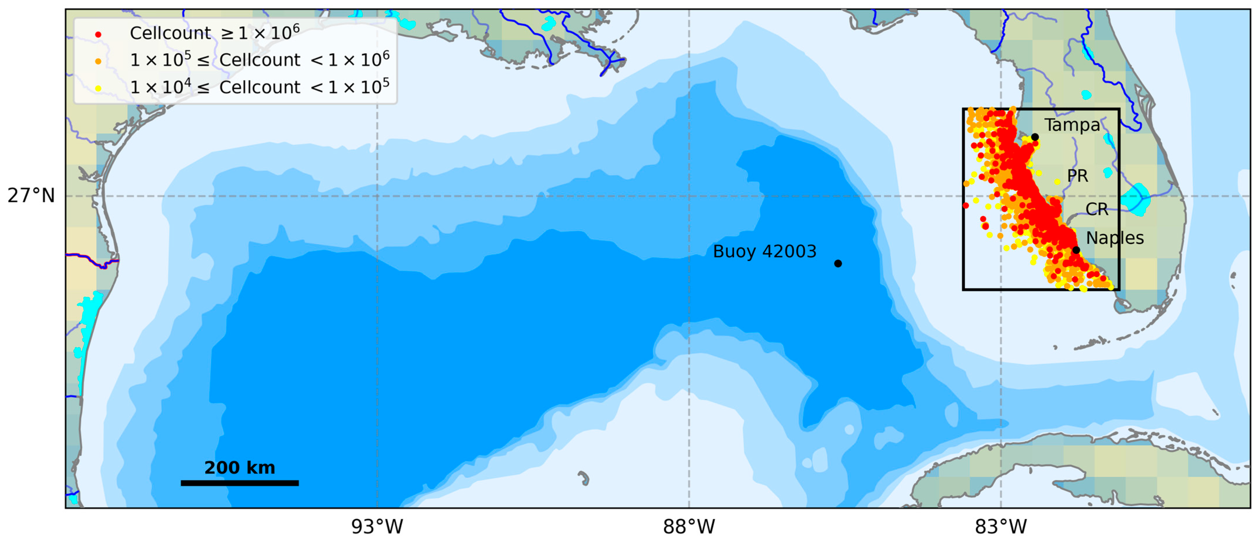
The study domain (Figure 1) focuses on the southwest Florida coastal region, specifically nearshore waters influenced by the Peace River and Caloosahatchee River watersheds, extending from Charlotte Harbor to the Tampa Bay region [19]. This area was selected to capture coastal environments most directly impacted by terrestrial nutrient loading and shelf-scale physical forcing [39,40]. Observations of K. brevis cell concentrations were obtained from the Florida Fish and Wildlife Conservation Commission (FWC-FWRI) long-term monitoring database for the period between January 1990 and December 2024 [41]. To align K. brevis observations with environmental predictors, cell counts were aggregated to a weekly temporal resolution. For the machine-learning classification task, bloom presence was defined using a binary threshold of ≥100,000 cells L⁻¹, consistent with operational monitoring criteria and prior ecological studies [19,39,42]. Observations below this threshold were classified as non-bloom conditions. Spatial coordinates of sampling locations were used to associate biological observations with environmental data but were not explicitly included as predictive features in the machine learning model.

During the preparation of this manuscript/study, the authors used GPT-5.2 and Gemini 2.5 Pro to provide review comments, and to improve text clarity, succinctness, logical flow, and overall polish. Coding for data analysis and plotting was performed using Python (CPython, Python Software Foundation, version 3.12.8) with assistance from GPT-4o through Jupyter AI and GPT-5.2.

2.2. Physical Drivers

Sea surface temperature (SST) and salinity data were obtained from the same FWC-FWRI monitoring records used for the biological data, ensuring temporally aligned sampling [41]. These variables were aggregated to weekly maximum values to preserve episodic extremes, such as seasonal warming or freshwater pulses, that influence the physical and biogeochemical environment [40,43]. Wind speed and direction data were sourced from NOAA buoy 42003 on the West Florida Shelf [44]. Large-scale circulation variability associated with the Loop Current was represented using sea surface height (SSH) anomalies (zos). Daily gridded SSH data were obtained from the Copernicus Marine Environment Monitoring Service (CMEMS) global ocean physics product (GLOBAL_MULTIYEAR_PHY_001_030) at an ~8 km horizontal resolution [45,46]. SSH anomalies were spatially averaged across the Gulf of Mexico domain and detrended to isolate high-frequency fluctuations associated with Loop Current excursions and eddy activity [47]. Both contemporaneous and lagged SSH values were included to account for the delayed physical response of coastal waters to basin-scale circulation forcing.

Wind vectors were converted to zonal (u) and meridional (v) components and vector-averaged to weekly mean values. Lagged wind predictors were then constructed by shifting these weekly time series by one- and two-week intervals to account for the delayed response of surface currents and bloom transport to atmospheric forcing, lagged wind variables were computed at weekly intervals, reflecting documented wind-driven circulation timescales [48,49]. Satellite-derived datasets were considered for multiple physical drivers; however, limitations in temporal alignment within situ biological observations constrained their inclusion in the present analysis. Future work could incorporate remote sensing products to enhance spatial coverage and improve model generalizability.

2.3. River Discharge and Nutrient Loading

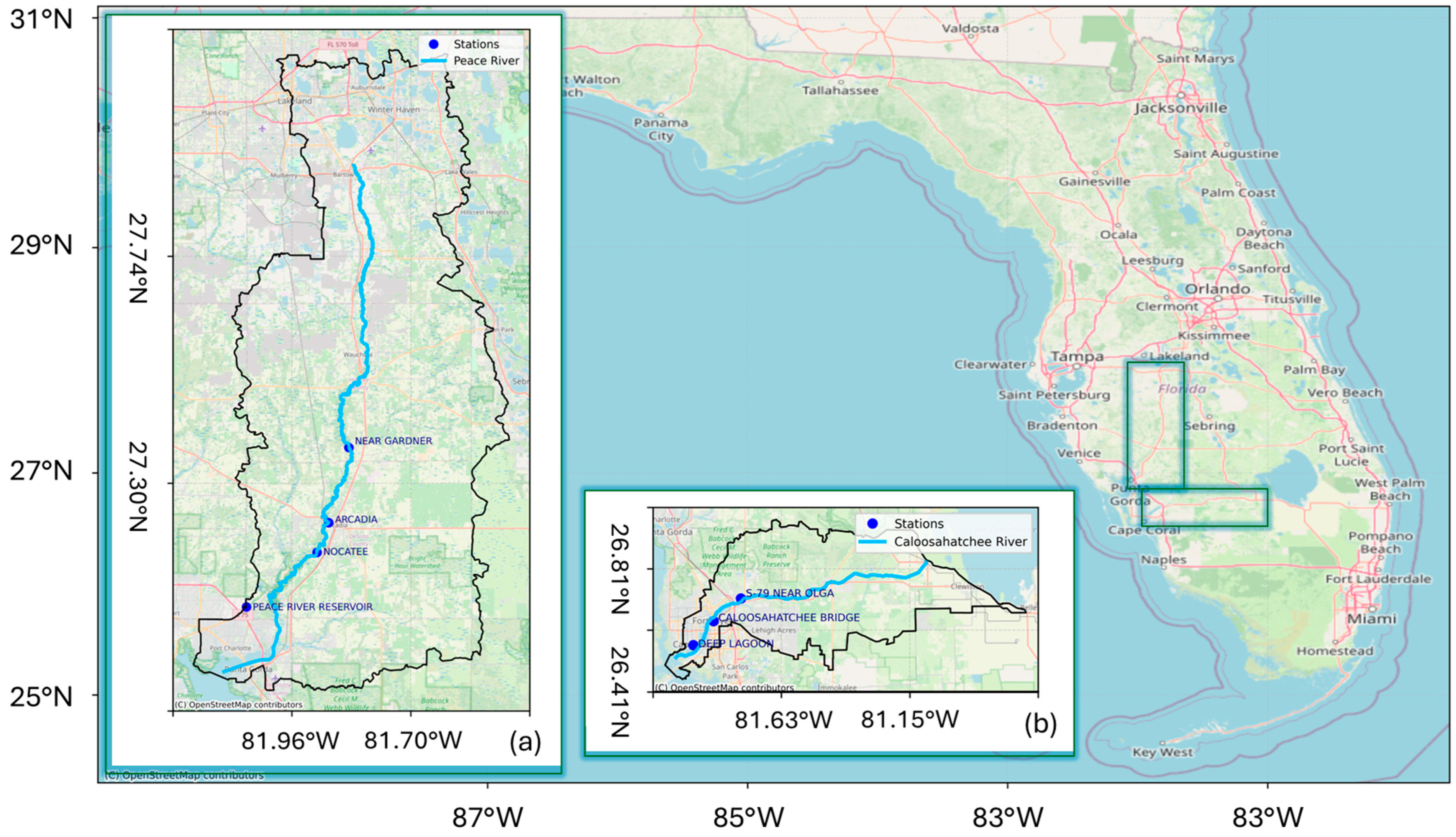
Land-based freshwater and nutrient inputs were quantified for the Peace and Caloosahatchee Rivers, the primary sources of nitrogen and phosphorus to the region [7,18]. For the Peace River (Figure 2a), daily discharge data were obtained from U.S. Geological Survey (USGS) gauging stations near Bartow and Arcadia, and corresponding total nitrogen (TN) and total phosphorus (TP) concentrations were retrieved from the Water Atlas of Florida [50]. For the Caloosahatchee River (Figure 2b), discharge data were sourced from the S-79 flow control structure, which serves as the primary freshwater delivery point to the estuary. Nutrient data (TN and TP) for the Caloosahatchee were obtained from the Florida Storage and Retrieval (STORET) database and the Water Quality Portal [51]. Details about data curation procedures for discharge and nutrient data of Peace River and Caloosahatchee River are provided in publicly available data repositories. For both river systems, discharge and nutrient concentration data were resampled to a weekly resolution. Weekly maximum values were retained to capture the episodic high-flow pulses and high-concentration that have been shown to exert a disproportionate influence on coastal phytoplankton dynamics [7,15,19]. Lagged predictors for discharge and nutrients were also constructed to represent delayed biological responses to watershed forcing.

2.4. Combined Environmental Dataset

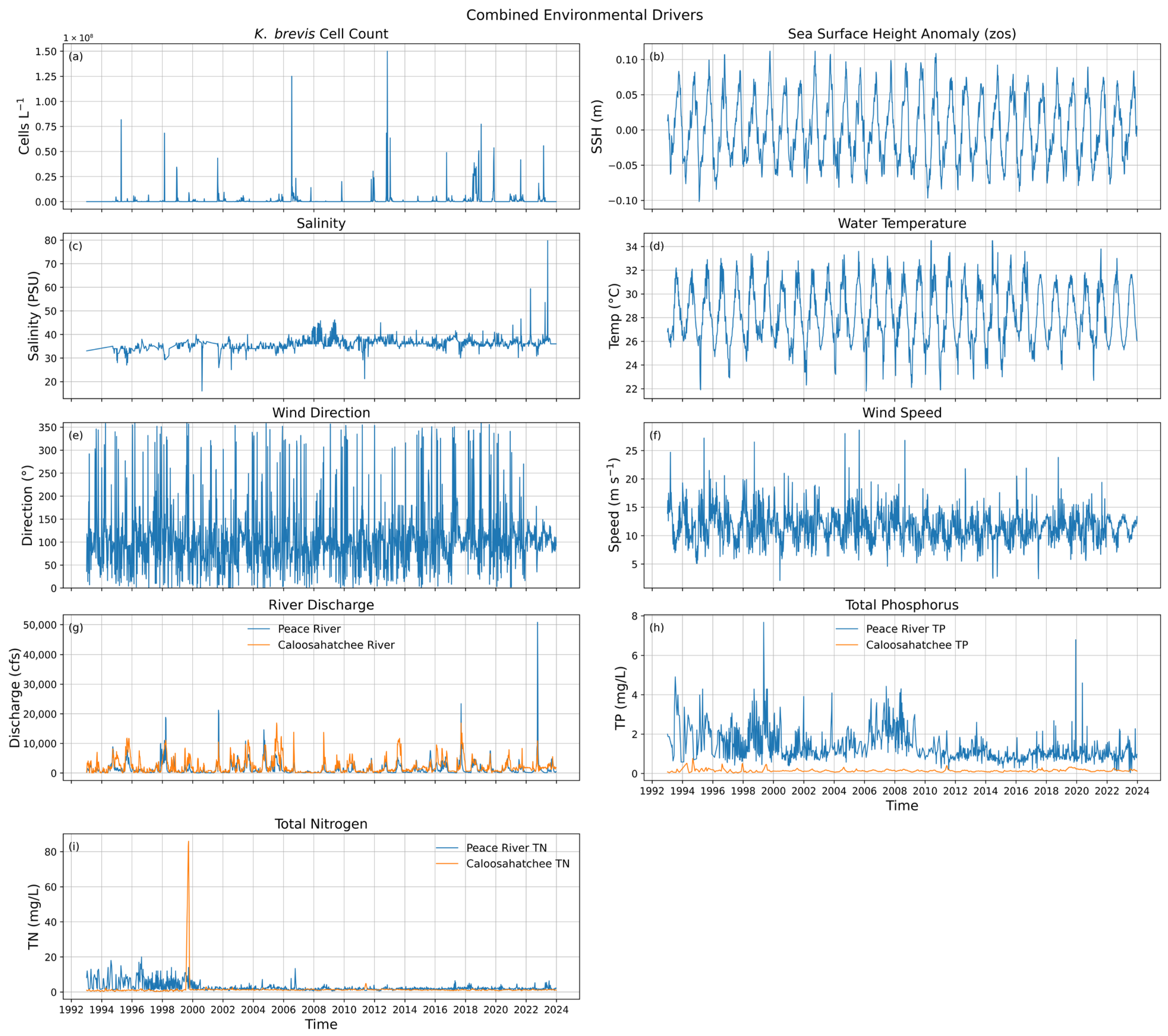
All biological and environmental variables were integrated into a single, temporally aligned dataset to serve as the feature matrix for machine learning. K. brevis cell counts, salinity, and water temperature were aggregated into weekly intervals using maximum values to preserve physiological and environmental extremes [40]. Physical drivers, including wind vector components and sea surface height (SSH) anomalies, were aggregated into weekly means to represent persistent forcing conditions. Environmental datasets associated with the Peace River basin including river discharge and nutrient concentrations were merged with oceanographic and atmospheric variables on a common weekly time index. Corresponding weekly discharge and nutrient data for the Caloosahatchee River were processed separately and subsequently joined to the Peace River dataset using an outer join on the time variable. This approach preserved the full temporal coverage of both river systems while allowing for asymmetric data availability across watersheds. Following dataset integration, rows containing missing values across predictor variables were removed to ensure a complete feature matrix for model training and evaluation. This listwise deletion was applied after all lagged predictors were constructed to avoid partial feature vectors. The final integrated dataset for machine learning training and validation, providing a multi-decadal record of biological responses and regional drivers, is summarized in Figure 3 and detailed in publicly available data repositories [52,53].

2.5. Machine Learning Framework

K. brevis bloom occurrence was treated as a binary classification task. Model predictions target weekly bloom occurrence one week ahead ($t+1$), using predictor information available at week t, including contemporaneous environmental variables and lagged terms. A threshold of ≥100,000 cells L⁻¹ was applied to define the “bloom” class, with all other values designated as “non-bloom” [42]. To evaluate the influence of expanded spatial sampling on model performance, the K. brevis response record was expanded to include coastal bloom observations from the Tampa Bay region. Tampa Bay observations were merged into the dataset as an additional bloom observation time series; however, model targets were defined using the Southwest Florida K. brevis record (kb) and the integrated environmental predictors. This augmentation increased spatial coverage of bloom occurrence and improved temporal continuity of the concentration record, while retaining the same environmental predictor framework. The dataset was split chronologically to preserve temporal structure and prevent information leakage. All observations prior to 1 January 2019 were used for model training, while a contiguous holdout period from 2019 onward was reserved exclusively for testing. Each sample represents a single weekly observation (one row per week) formed by merging regionally compiled bloom observations and environmental predictors on a common weekly time index. All predictor variables were normalized prior to model training, and K. brevis cell counts were converted to a binary bloom classification (≥100,000 cells L⁻¹), such that the model inputs are directly derived from the time series presented in Figure 3. No random shuffling was applied. Feature scaling was performed using a RobustScaler fit only on the training data and applied to the test data; although tree-based models are generally insensitive to scaling, this approach improves numerical stability and ensures consistency across predictors with differing units and distributions.

The primary predictive model was a Random Forest (RF) classifier, selected for its ability to capture non-linear interactions, handle collinearity among predictors, and provide robust performance for complex and potentially noisy environmental datasets, while reducing susceptibility to overfitting [37]. The model was implemented using 100 trees (n_estimators = 100), with class balancing and a fixed random state (random_state = 42), while all other hyperparameters (e.g., maximum tree depth, minimum samples per split, and number of features considered at each split) were set to their default values in scikit-learn, which provided stable performance without additional tuning. To account for biological persistence and the local retention of biomass, lagged predictors (one- and two-week intervals) were constructed for K. brevis cell counts and watershed inputs [16]. To address class imbalance (the prevalence of non-bloom weeks over bloom weeks), class-weighted model fitting was implemented to ensure the minority bloom class contributed proportionally during the training phase [37]. Predictor variables were scaled using a normalization approach based on the median and interquartile range to reduce sensitivity to hydrological and nutrient extremes as detailed in [52]. The supervised classification model was evaluated within a common preprocessing framework. Models were implemented using established open-source machine learning libraries including scikit-learn using default hyperparameter settings [54]. Model performance was evaluated using a temporally separated test set and supported by learning curve analysis to assess generalization performance.

2.6. Model Evaluation and Interpretability

Model performance was evaluated on a withheld test subset using metrics optimized for imbalanced environmental data. These included balanced accuracy, which averages sensitivity and specificity, and the F1-score, which provides a harmonic mean of precision and recall [34,37]. Performance metrics were calculated using standard confusion matrix definitions true positives (TP), false positives (FP), true negatives (TN), and false negatives (FN). Accuracy is defined as

$$\mathrm{Accuracy}={\displaystyle \frac{\mathrm{TP}+\mathrm{TP}}{\mathrm{TP}+\mathrm{TN}+\mathrm{FP}+\mathrm{FN}}}$$

(1)

to measure the overall percentage of correct predictions. Precision is defines as

$$\mathrm{Precision}={\displaystyle \frac{\mathrm{TP}}{\mathrm{TP}+\mathrm{FP}}}$$

(2)

to quantify the proportion of predicted bloom events that were correctly identified, reflecting the model’s ability to minimize false-positive bloom predictions. Recall (sensitivity or true positive rate) is defined as

$$\mathrm{Recall}={\displaystyle \frac{\mathrm{TP}}{\mathrm{TP}+\mathrm{FN}}}$$

(3)

to measure the proportion of observed bloom events that were correctly detected, indicating the model’s sensitivity to bloom occurrence. Similarly, specificity is defined as

$$\mathrm{Specificity}={\displaystyle \frac{\mathrm{TP}}{\mathrm{TP}+\mathrm{FN}}}$$

(4)

The F1-score, defined as the harmonic mean of precision and recall

$$\mathrm{F}1=2{\displaystyle \frac{\mathrm{Precision}·\mathrm{Recall}}{\mathrm{Precision}+\mathrm{Recall}}},$$

(5)

provides a balanced measure of bloom prediction performance under class imbalance. Therefore, a high F1-score means the model achieves a good balance between precision and recall.

The receiver operating characteristic area under the curve (ROC–AUC) evaluates the model’s ability to distinguish between bloom and non-bloom conditions across all classification thresholds. The ROC curve and corresponding AUC were explicitly computed to provide a threshold-independent assessment of model discrimination. Balanced accuracy calculated as

$$\mathrm{Balanced} \mathrm{Accuracy}={\displaystyle \frac{\mathrm{Sensitivity}+\mathrm{Specificity}}{2}}$$

(6)

computes the mean of sensitivity (how well the model detects bloom events) and specificity (how well the model correctly identifies non-bloom conditions). Thereby balanced accuracy accounts for class imbalance by equally weighting bloom and non-bloom classification performance. Additionally, the Youden index

$$J=\mathrm{Sensitivity}+\mathrm{Specificity}-1$$

(7)

assesses the trade-off between bloom detection and false-alarm rates. The Youden index was further used to identify the optimal classification threshold that maximizes the combined sensitivity and specificity. All metrics were computed directly from the held-out test dataset using scikit-learn. Model interpretability was assessed using permutation-based feature importance, quantifying the sensitivity of the model’s predictive skill to individual environmental drivers implemented using standard routines in scikit-learn [54]. Partial dependence plots were utilized to visualize the marginal effects of river discharge and nutrient concentrations on bloom probability, as conditional model responses rather than mechanistic thresholds. Feature importance rankings and partial dependence plots were used to interpret model behavior by quantifying the relative influence of predictors and illustrating their effects on bloom probability.

3. Results and Discussion

3.1. Characterization of Regional Environmental Drivers

The integrated multi-decadal record (1990–2024) of environmental predictors and biological responses is illustrated in Figure 3, which highlights the temporal alignment of K. brevis cell counts with physical and biogeochemical forcing. The compiled dataset reveals episodic, high-magnitude nutrient loading and river discharge events that are characteristic of the southwest Florida coastal system [7]. These pulses are particularly evident in the late 1990s and during active hurricane seasons. This reflects the preservation of short-duration loading events that have been shown to exert a disproportionate influence on coastal phytoplankton dynamics [15,19]. Hydrographic conditions recorded concurrently with biological samples demonstrate clear seasonal variability, as shown in the publicly available data repository [53]. Salinity minima typically coincide with seasonal rainfall and high river discharge from the Peace and Caloosahatchee Rivers, which deliver elevated nitrogen and phosphorus loads to the nearshore environment [7,40]. Conversely, peak K. brevis cell counts often occur during periods of elevated water temperatures in late summer and fall, consistent with the physiological optima for the species [19,55].

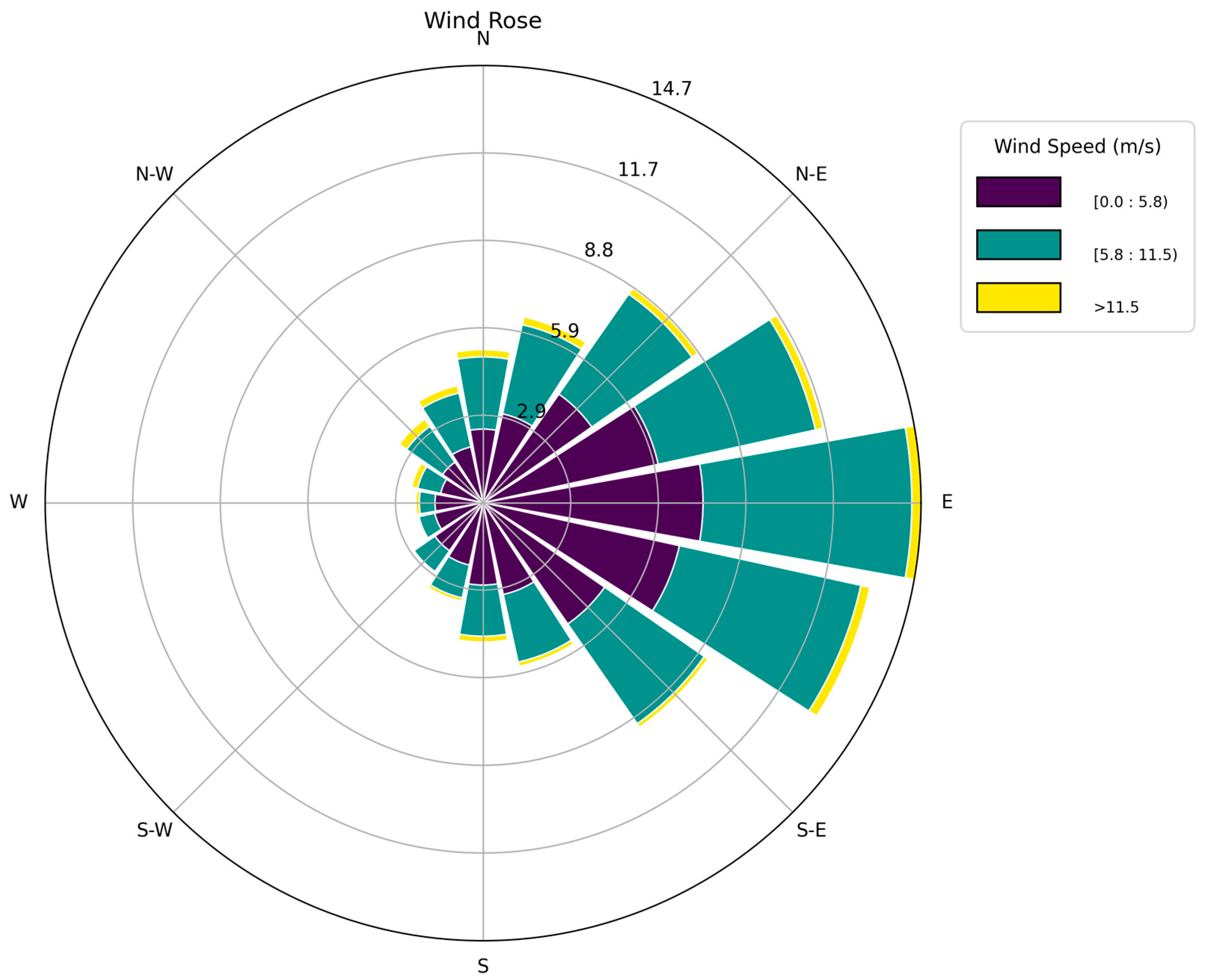
Physical forcing on the West Florida Shelf is further characterized by wind and circulation patterns. The wind rose in Figure 4 illustrates the distribution of wind vectors at NOAA buoy 42003, revealing a dominance of northeasterly and southeasterly components that reflect the regional seasonal atmospheric variability on the shelf. While this dataset provides consistent measurements of regional wind forcing, it may not fully capture localized variability. This spatial mismatch could contribute to a slight underestimation of wind-related feature importance. Nevertheless, the buoy data remain representative of broader atmospheric patterns influencing coastal transport and bloom dynamics. Future work could incorporate higher-resolution or nearshore wind observations to improve spatial specificity. Northerly wind components facilitate coastal upwelling and are associated with shoreward transport of blooms initiated offshore [47,49]. Furthermore, westerly (onshore) wind components play a vital role in bloom retention by preventing algal biomass from dispersing offshore and instead trapping nutrient-rich water against the coastline [37,55]. This shoreward retention can maintain elevated nearshore cell concentrations and is associated with increased respiratory irritation risk, as onshore winds facilitate the transport of aerosolized brevetoxins onto inhabited beaches [55]. Conversely, the frequent offshore easterly winds observed in the wind rose often correspond with reduced coastal exposure, transporting surface blooms away from the coast and reducing public health impacts even when high biomass is present in the study area [47,55]. Large-scale circulation, represented by sea surface height (SSH) anomalies, captures the variability of the Loop Current. Positive SSH anomalies reflect the northward penetration of the Loop Current, a physical configuration that has been associated with large-scale red tide manifestation along the southwest Florida coast [47,49,56].

3.2. Model Predictive Performance

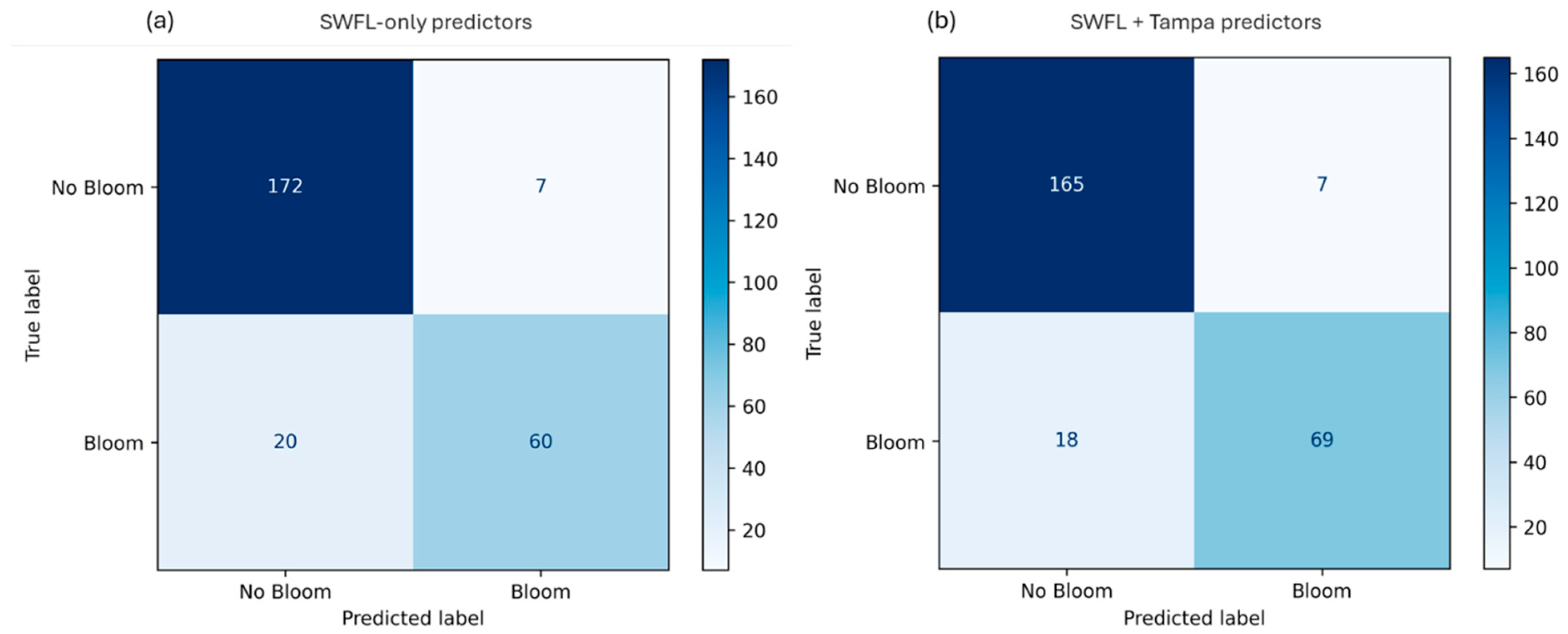
The Random Forest classifier demonstrated strong skill in predicting K. brevis bloom occurrence, achieving an overall accuracy of 90% and a balanced accuracy of 87.6%. For the final Random Forest model evaluated on the chronologically withheld test set (n = 259), the confusion matrix yielded TP = 69, TN = 165, FP = 7, and FN = 18. These values correspond to an accuracy of 0.903 (Equation (1)), precision of 0.908 (Equation (2)), recall of 0.793 (Equation (3)), F1-score of 0.847 (Equation (5)), and balanced accuracy of 0.876 (Equation (6)). The high precision (0.91) indicates that predicted bloom events are rarely false positives, while the recall (0.79) reflects the model’s ability to detect the majority of observed bloom events. The F1-score and balanced accuracy provide complementary measures that balance detection performance across imbalanced bloom and non-bloom classes. These metrics are consistent with strong combined sensitivity and specificity (i.e., high Youden index). Reliable performance across both bloom and non-bloom classes is a critical requirement for this framework, given the inherent class imbalance found in multi-decadal biological monitoring records [34,37]. For the minority bloom class (≥100,000 cells L⁻¹), the model reached an F1-score of 0.847, supported by high precision (91%) and recall (79%). As illustrated in the Confusion Matrix (Figure 5), the model correctly identified 165 out of 172 true non-bloom weeks and 69 out of 87 true bloom weeks, indicating an ability to distinguish between bloom and non-bloom conditions while minimizing both missed events and false alarms.

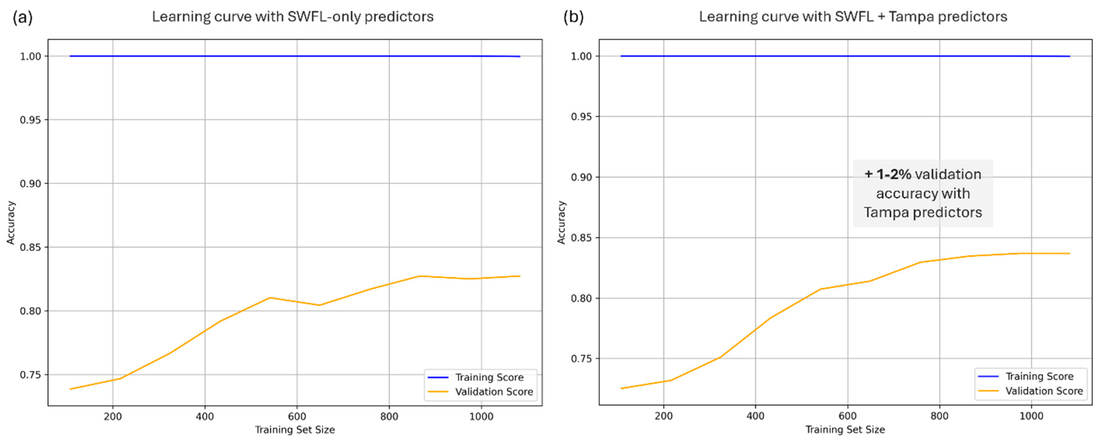
Model generalization and the impact of data density were evaluated using the learning curve (Figure 6). Validation accuracy increased steadily with training set size before plateauing near 84%. While the model achieved a training accuracy of 1.00 across all sample sizes, reflecting strong memorization capacity, the persistent generalization gap between training and validation scores suggests a tendency toward overfitting. Exposure to a broader range of bloom and non-bloom conditions through additional observations was associated with improved model sensitivity, though the leveling of validation accuracy near 84% indicates that predictive performance remains constrained by data availability and variability. Historical bloom records are inherently imbalanced, with substantially more non-bloom weeks than bloom weeks. Although class weighting and feature engineering helped address this imbalance, further improvement may be achieved by incorporating additional observations or satellite-derived bloom proxies to increase the density of bloom-related data [32,57].

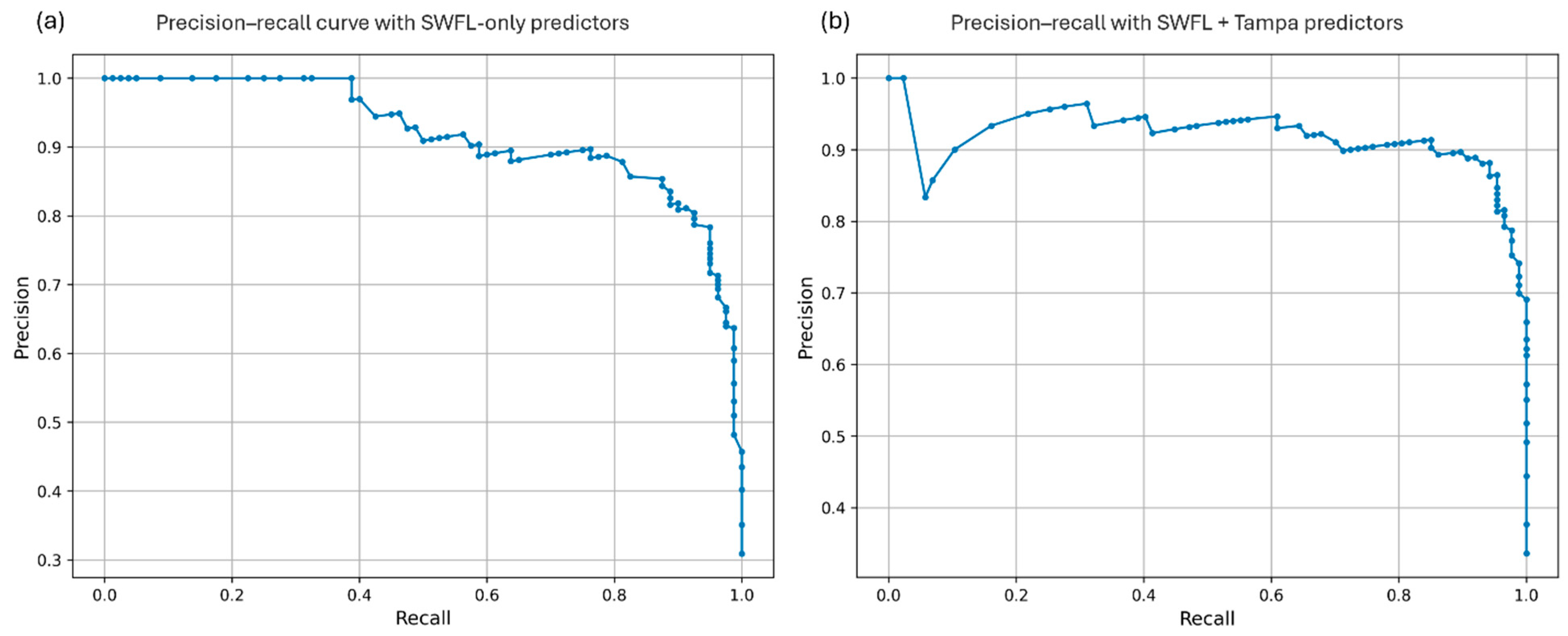
The stability of the classification threshold was further assessed using the precision–recall curve (Figure 7). The classifier maintained strong precision (~0.90) as recall increased toward ~0.80, with a notable performance drop occurring only at the highest recall levels (>0.90). This trade-off is characteristic of imbalanced environmental classification problems, where aggressively attempting to capture all bloom events increases false-positive predictions [37]. Overall, the model’s ability to capture the timing and persistence of bloom activity with high consistency demonstrates the effectiveness of the regionally integrated machine learning framework for short-term bloom occurrence prediction. The non-monotonic patterns observed in the precision–recall curves in Figure 7 reflect the data-driven nature of the Random Forest model and the discrete evaluation of classification thresholds. Such behavior is expected in imbalanced environmental classification problems and should be interpreted as a realistic representation of the trade-offs between precision and recall, rather than as a smooth functional relationship.

A distinguishing aspect of this study is the integration of nutrient data from both the Peace and Caloosahatchee Rivers into a single predictive framework. Previous analyses often focused on a single watershed, whereas this approach captures a broader representation of nutrient dynamics across southwest Florida. By incorporating data from both rivers along with bloom observations from Tampa Bay, the model reflects the combined influence of multiple freshwater sources. This regional scope may have contributed to improved predictive robustness compared to localized models [58,59]. The findings suggest that predictive performance benefits from a multi-watershed perspective that captures cumulative nutrient forcing. Although this study focuses on southwest Florida, the approach could be adapted to other regions with complex freshwater–coastal interactions, such as estuaries or river plume systems, provided that sufficient historical records are available [2,37]. This pattern reflects the importance of watershed–coastal coupling processes, where riverine inputs interact with coastal physical conditions to regulate bloom dynamics.

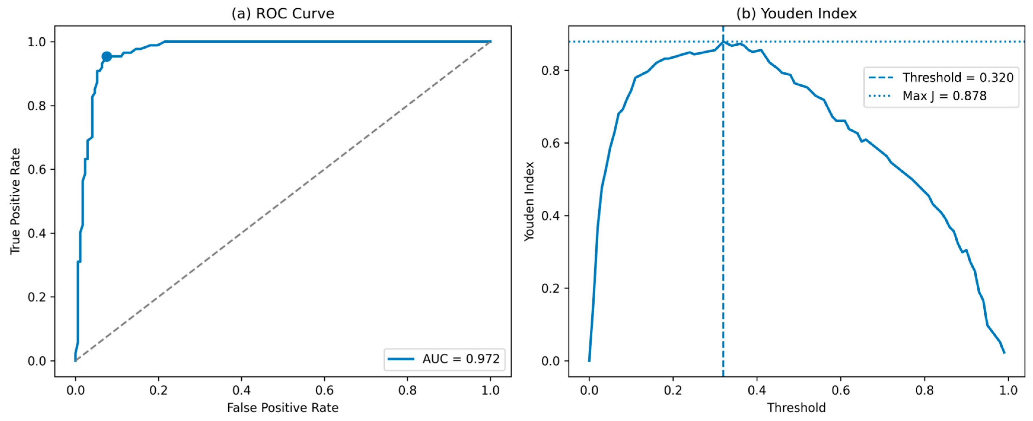
In addition, the receiver operating characteristic (ROC) curve further demonstrates strong classification performance (Figure 8a), with an area under the curve (AUC) of 0.972, indicating excellent discrimination between bloom and non-bloom conditions across classification thresholds. Analysis of the Youden index (Figure 8b) identified an optimal classification threshold of 0.320, corresponding to a maximum Youden index of 0.878, reflecting a strong balance between sensitivity and specificity. These results complement the threshold-dependent metrics by providing a threshold-independent assessment of model performance and confirming the robustness of the selected classification framework.

3.3. Biological Persistence and Influence of Lagged Features

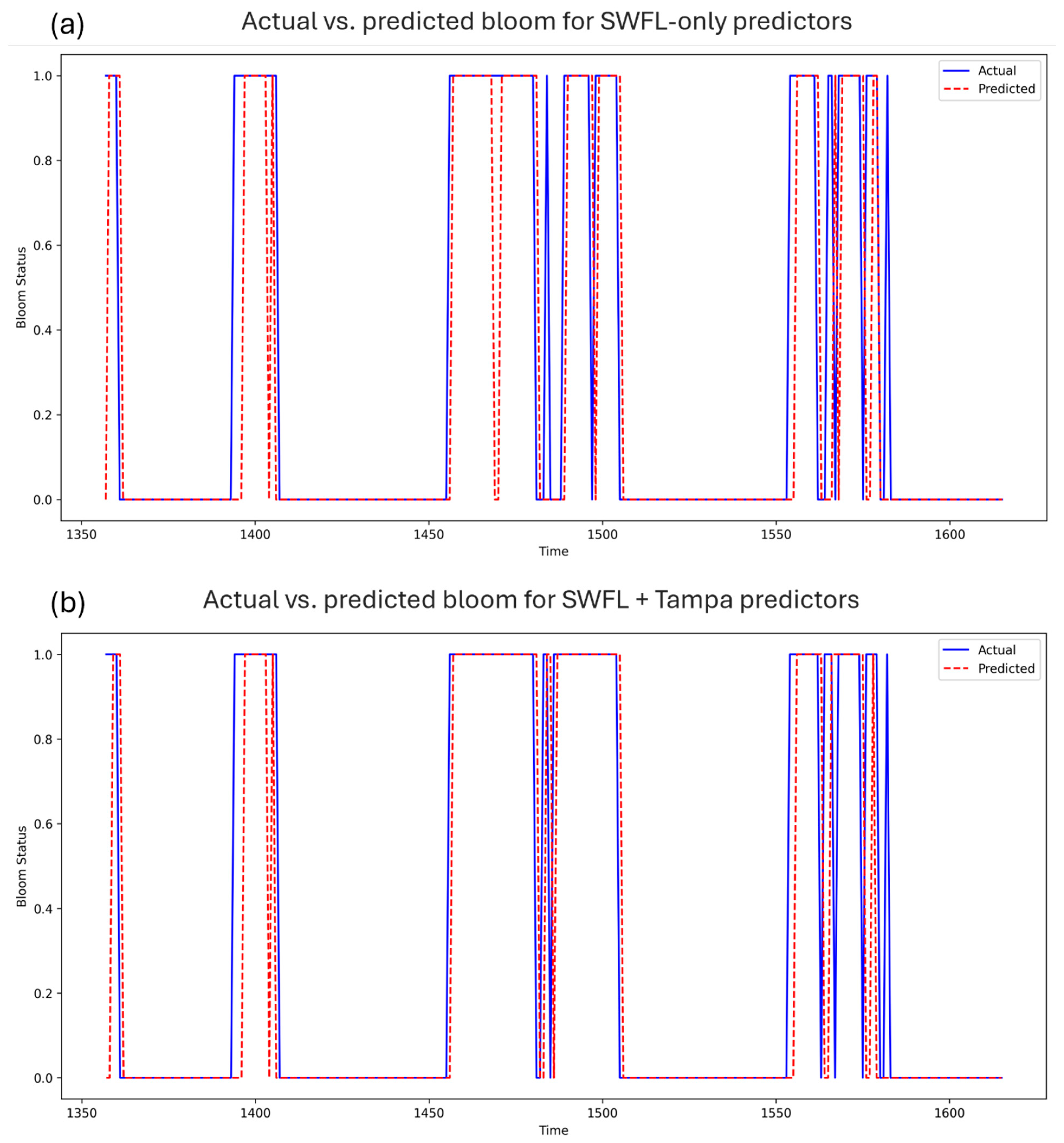
A significant factor in the strong predictive skill of the Random Forest model was the inclusion of lagged biological predictors, specifically K. brevis cell concentrations from the preceding one and two weeks. As shown in Figure 9, the model’s predicted bloom status closely tracks the timing and duration of actual events, showing strong agreement during ongoing bloom periods. This performance during sustained events reflects the fact that coastal blooms do not dissipate instantaneously. Instead, they persist through a combination of biological continuity, local retention of biomass, and shelf-scale advection. In this context, lagged predictors function as indicators of short-term persistence rather than independent environmental forcing. However, the model’s reliance on these autoregressive features can introduce a potential weakness in detecting abrupt bloom emergence, defined as transitions from a non-bloom state to a bloom state following an extended period of absence. As illustrated by the “Actual Versus Predicted” comparison in Figure 9, while the model identifies bloom start dates with minimal lag, its sensitivity may be reduced in scenarios where recent bloom history is absent. This reflects a common challenge in machine learning for HABs, where models may learn to repeat the most recent observation as a shortcut to high accuracy, essentially “catching up” to reality rather than providing a leading indicator of initiation. Thus, while the model excels at short-term operational forecasting, its skill would likely decrease for long-lead initiation forecasts if biological lags were excluded. Accordingly, the current model-structure prioritizes predictive reliability for ongoing public health threats over mechanistic initiation modeling. Future sensitivity experiments that isolate environmental drivers from biological lags are warranted to quantify the relative contribution of external forcing such as nutrient loading and wind-driven transport during the critical onset phase. Despite this limitation, the Random Forest architecture utilized here remains more robust for this data structure than simple linear models, which fail to capture the nonlinear threshold effects inherent in biological persistence. As such, while the current framework demonstrates strong predictive performance, it does not explicitly disentangle the relative contributions of environmental drivers and autoregressive biological signals, and model skill should be interpreted in the context of this limitation.

3.4. Synergistic Effects of Nutrient Loading and Discharge

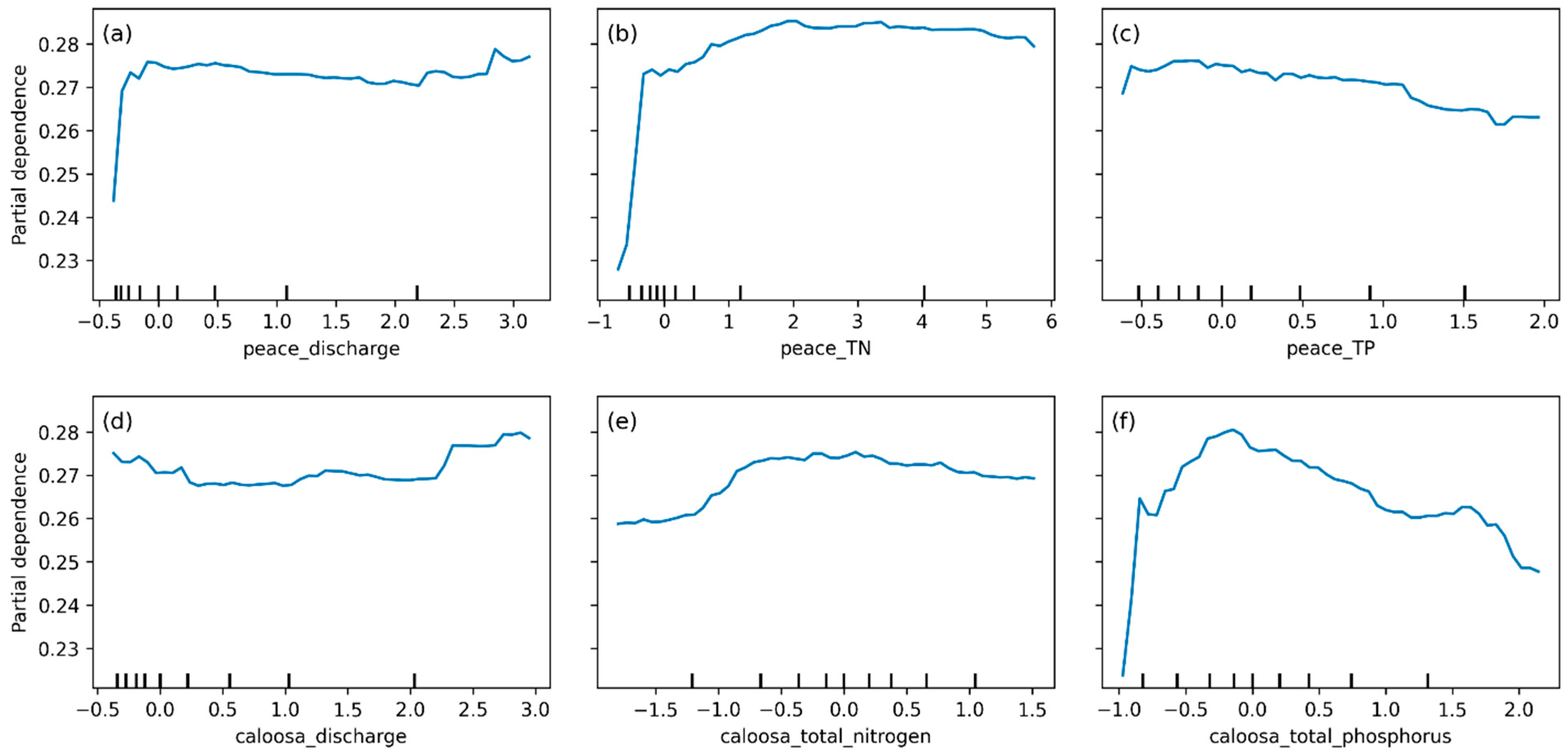
While physical forcing governs the transport and retention of biomass, the intensity and duration of coastal blooms are associated with the availability of nutrients [7,16]. The Random Forest model identified nonlinear relationships between watershed inputs and bloom probability, as illustrated by the partial dependence plots (Figure 10). Contrary to a simple linear dose–response relationship, the model indicates that bloom probability rises sharply with low-to-moderate increases in river discharge and total nitrogen (TN) concentrations before plateauing or slightly declining at the highest values. This plateau suggests a model-inferred saturation range, which is approximately 2–3 mg L⁻¹ for TN and 1.5 mg L⁻¹ for Total Phosphorus (TP), beyond which additional loading does not proportionally increase bloom risk. Hydrological conditions, particularly discharge from the Peace and Caloosahatchee Rivers, were also key drivers of bloom probability. The model indicates that moderate discharge events, often following seasonal rainfall or runoff pulses, are associated with elevated bloom probability.

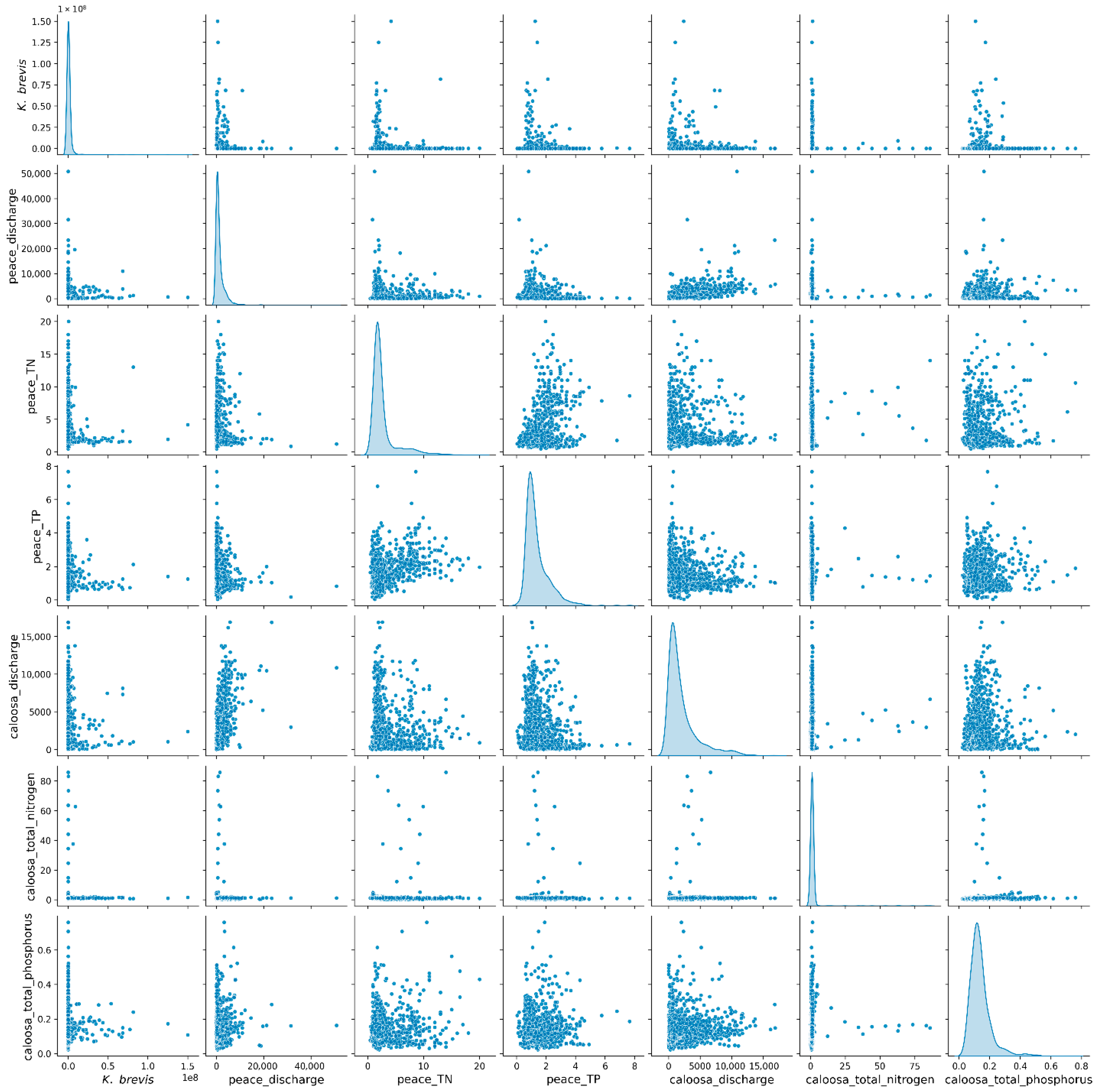
Consequently, K. brevis blooms were most strongly associated with moderate, rather than extreme, nutrient inputs and river discharge. Pairwise relationships among environmental variables (Figure 11) indicate that blooms tend to occur when TN and TP are elevated but not extreme. This pattern is consistent with nutrient threshold behavior or co-limitation effects [59,60], where blooms are supported within a narrow range of nutrient availability but are suppressed by very low or excessively high concentrations [2,17].

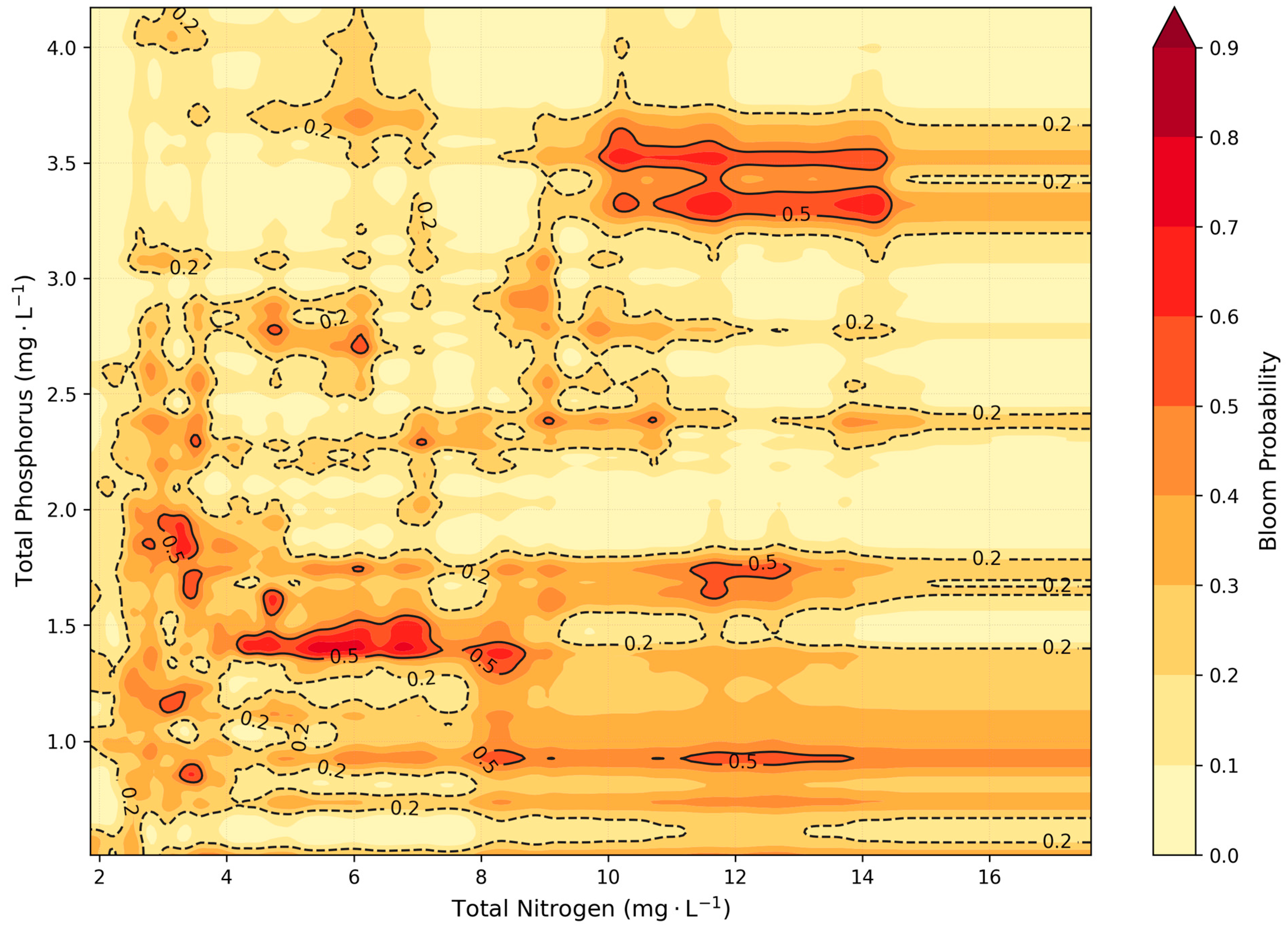
The interactions between specific nutrients were further examined using probability contour plots (Figure 12), which indicate a synergistic association between nitrogen and phosphorus availability. Bloom probability remains relatively low when either TN or TP concentrations are minimal, but increases substantially when both are elevated simultaneously. Specifically, the highest modeled probabilities (>0.6) occur when TN exceeds ~8–10 mg L⁻¹, and TP exceeds ~ 1.5 mg L⁻¹. These results are consistent with prior evidence that K. brevis blooms on the West Florida Shelf may reflect balanced nutrient stoichiometry and co-limitation rather than control by a single limiting nutrient [2,7,14,17,19,60].

The lack of a consistent correspondence between extreme discharge events and bloom occurrence suggests that freshwater inflow may sometimes dilute or disperse blooms rather than intensify them [61]. Large discharge events can also lower nearshore salinity below levels favorable for K. brevis growth (~24 ppt), further limiting bloom development [62]. This nonlinearity reflects the complex interaction between hydrology, salinity, and nutrient delivery, and indicates that river inputs play a dual role in bloom dynamics depending on timing and magnitude. For example, while riverine discharge delivers essential nutrients, extreme flow events can reduce the local residence time necessary for algal accumulation, effectively flushing biomass from the estuary [61,63]. Potential alternate explanations for the observed relationships can be considered. For example, correlations between river discharge and bloom events may reflect broader seasonal patterns rather than direct nutrient effects [64]. Offshore nutrient sources, such as nitrogen fixation or upwelling, were not accounted for, and these processes could play a role in sustaining blooms during certain seasons [17,61]. Future models that integrate offshore nutrient data may provide a more complete picture of bloom dynamics.

However, caution is required when interpreting these nutrient-bloom associations. As shown in the pairwise relationship plot (Figure 12), the distributions of nutrient data are strongly right-skewed, meaning that extreme high-nutrient events are rare in the training record. Recent analyses have reported positive relationships between Caloosahatchee River TN loading and K. brevis bloom severity or duration across both long-term records and recent bloom periods [13,65], suggesting that increased watershed nitrogen inputs can enhance bloom persistence once populations are established nearshore. In contrast, the present machine-learning analysis indicates a nonlinear response, with peak bloom probabilities occurring at moderate nutrient levels, followed by an apparent plateau at higher concentrations. However, because extreme nutrient and discharge conditions are sparsely represented in the dataset, this saturation-like behavior may partly reflect limited data coverage at the upper range rather than a true ecological threshold, and predictive uncertainty correspondingly increases under these conditions. Furthermore, while the model successfully uses nearshore nutrient concentrations as predictors, this does not confirm a strictly causal “bottom-up” driving mechanism. Elevated nutrient concentrations within a bloom may be partly a result of the bloom itself, generated through biological regeneration, zooplankton excretion, and the decay of fish kills, rather than solely representing external watershed loading [19,66,67]. Therefore, while the machine learning framework confirms that watershed discharges are strong predictors of bloom maintenance and intensification in the nearshore environment [7], they should not be interpreted as primary drivers of offshore bloom initiation [68,69].

3.5. Role of Physical Forcing

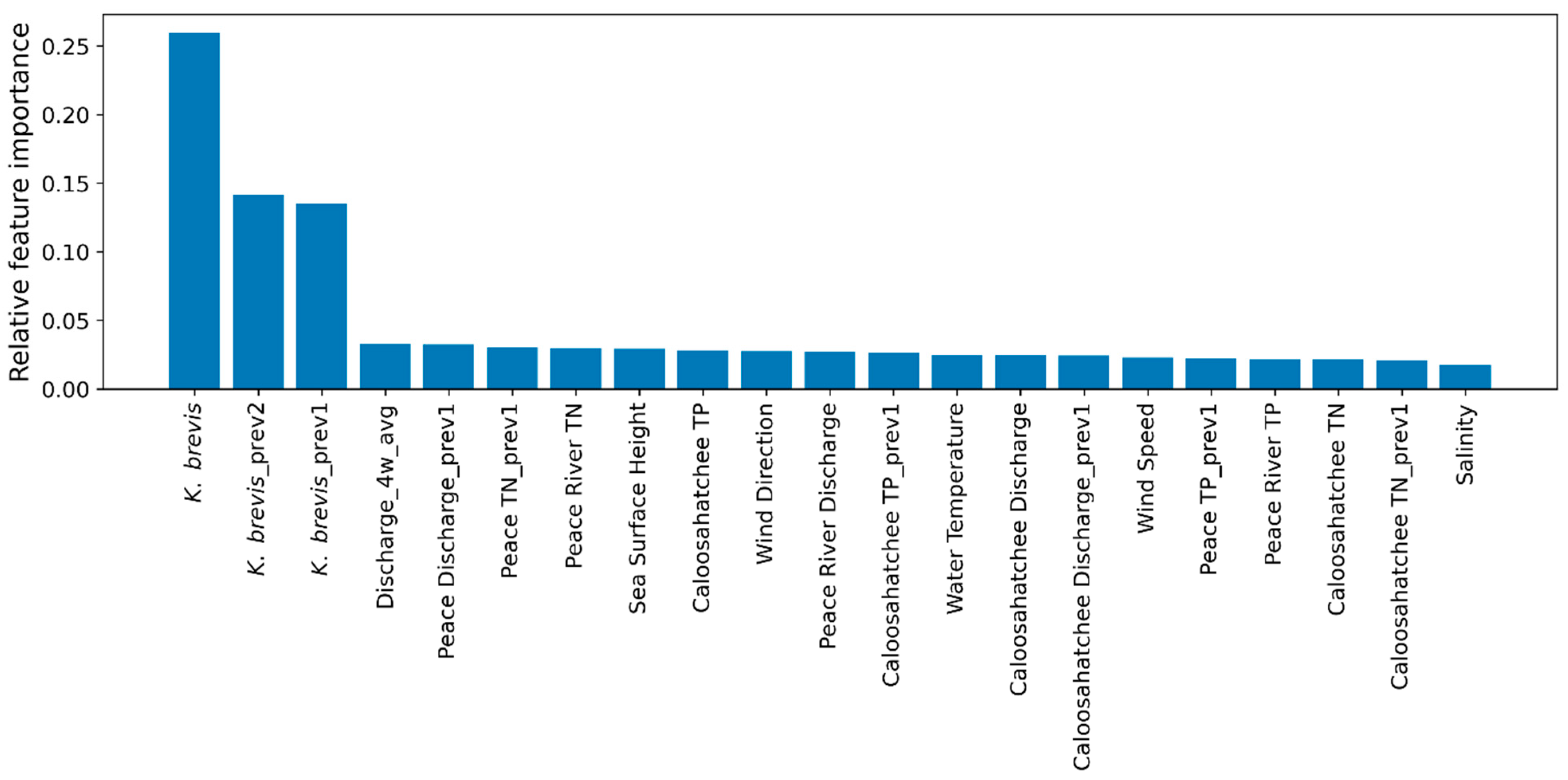
While biological persistence and nutrient availability emerged as the dominant predictors in the Random Forest model, physical oceanographic variables—specifically wind forcing and sea surface height (SSH) anomalies—retained moderate importance, acting as essential modulators of bloom transport and maintenance. As indicated in the feature importance ranking (Figure 13), wind speed and direction were secondary to riverine inputs but consistently contributed to model accuracy. This ranking aligns with the prevailing bloom hypothesis, where physical forcing is not the primary source of biomass generation but is the critical mechanism for delivering offshore-initiated populations to the nearshore environment [68,70]. The model’s sensitivity to wind direction reflects the physical necessity of onshore and downwelling-favorable winds for concentrating K. brevis cells against the coast. Periods of onshore winds can retain nutrient-rich water nearshore, creating conditions favorable for bloom maintenance [48,71]. Analysis of the wind rose (Figure 4) confirms that easterly winds are the prevailing wind direction on the West Florida Shelf. However, model sensitivity analysis indicates that less frequent westerly and southwesterly wind events are associated with accumulation of surface populations in the surf zone, a process documented to intensify respiratory irritation events [55]. Conversely, persistent easterly (offshore-directed) winds tend to disperse surface blooms seaward, reducing nearshore severity even if the bloom persists offshore [49,61]. Future work could examine these atmospheric effects more directly, particularly their interaction with coastal circulation and transport.

The influence of the Loop Current, represented by SSH anomalies, was captured by the model but ranked lower than watershed variables (Figure 13). While positive SSH anomalies (indicative of a northward Loop Current extension) have been statistically associated with increased retention of waters on the West Florida Shelf, a condition favorable for bloom maintenance [49], the modest influence of SSH within the model indicates that complex shelf interactions controlling bloom persistence may not be fully resolved using surface elevation alone. The machine learning model may struggle to resolve the specific “pressure point” interactions at the shelf slope [47,61]. These interactions drive deep-layer upwelling that can either fuel blooms or, in cases of extreme duration (e.g., 2010), suppress them by flushing the shelf with excess inorganic nutrients that favor faster-growing diatoms over K. brevis [47,61].

The model exhibited weaker sensitivity to SST than expected, given that temperature can affect K. brevis growth rates [2]. One explanation is that SST shows relatively minor seasonal fluctuations in the Gulf compared to nutrient and discharge dynamics, making it a less prominent predictor on a weekly scale. Alternatively, temperature effects may be indirectly captured through correlated variables such as seasonal rainfall or runoff [71], or may act primarily as a background environmental condition that modulates bloom potential rather than serving as a direct short-term predictor [13]. Similarly, salinity, while important in bloom ecology, did not dominate the predictive signal, likely due to its strong correlation with discharge events already accounted for in the dataset [61].

3.6. Model Limitations

A notable limitation is that the model uses surface nutrient concentrations as proxies for bloom potential, while subsurface processes such as upwelling and benthic nutrient fluxes were not represented [61,71]. Biological factors, such as grazing pressure and competition with other phytoplankton, were also excluded. These processes can influence bloom development and persistence, particularly when environmental conditions are borderline favorable [1,2]. Adding biological or optical indicators such as chlorophyll-a concentrations or particulate matter data could improve predictive performance in future iterations [32,57,72]. In addition, the model does not explicitly represent key biological and ecological processes (e.g., microbial interactions, physiological responses, and trophic feedbacks). As such, it should be interpreted as identifying statistical relationships rather than resolving underlying ecological mechanisms. Furthermore, the use of weekly aggregated wind data may smooth out rapid, synoptic-scale wind events (e.g., frontal passages) that drive immediate biological responses. While the model effectively forecasts the maintenance of existing nearshore blooms based on nutrient and autoregressive signals, its ability to predict the initial onshore arrival of a bloom remains constrained by the lack of subsurface data. Future iterations incorporating outputs from hydrodynamic models (e.g., WFCOM) or subsurface glider data as features could significantly bridge this gap between surface proxies and 3D physical reality, including improved representation of circulation and residence time dynamics [14,61].

The Random Forest approach provided high accuracy and interpretability but does not explicitly model temporal dependencies between consecutive weeks. Instead, temporal structure was represented through the inclusion of lagged predictors, particularly recent K. brevis concentrations, which capture short-term biological persistence and local retention or redistribution of bloom biomass in coastal waters. Similar persistence-based effects have been noted in previous HAB modeling studies, where recent bloom history strongly influences near-term bloom probability [16,57]. While this strategy improves predictive skill during ongoing bloom conditions, it may reduce sensitivity to true bloom emergence events, defined as abrupt transitions from extended non-bloom periods to bloom conditions. In such onset scenarios, where bloom-history predictors are weak or absent, model predictions rely more heavily on external environmental forcing, including nutrient loading, river discharge, wind-driven transport, and ocean circulation variability. This limitation is consistent with prior findings that tree-based and autoregressive ML models tend to favor persistence over initiation dynamics and may struggle to capture abrupt bloom onset without explicit temporal sequence modeling [59,73]. Time-series–oriented approaches, such as recurrent neural networks or hybrid frameworks that explicitly encode temporal evolution, have therefore been proposed as complementary tools for improving bloom forecasting and the detection of emerging bloom conditions [57,74]. Future work should explicitly evaluate model performance with and without bloom-history predictors to quantify the relative contributions of persistence versus external environmental forcing, particularly for forecasting bloom emergence following extended non-bloom periods. Finally, while the model performed well on historical data, applying it operationally would require continuous updates to account for evolving climate and land-use patterns [2,75]. Changes in rainfall intensity, hurricane frequency, or sea-level rise could alter the historical relationships on which the model is based [1]. Periodic recalibration using recent data and scenario-based simulations could help ensure the model remains robust under changing environmental conditions. In addition, uncertainty in model performance metrics (e.g., confidence intervals) was not explicitly quantified in this study; incorporating such approaches in future work would provide a more complete assessment of model reliability.

Although the inclusion of Tampa Bay observations expands the environmental and biological variability represented during model training, explicit cross-regional validation was not performed in this study. As a result, the model’s ability to generalize across distinct coastal regions remains untested. Future work should evaluate transferability through cross-region validation experiments, such as training on one region and testing on another, to more rigorously assess spatial generalization.

4. Conclusions

This study developed a regionally integrated Random Forest machine learning framework for forecasting weekly K. brevis bloom occurrence on the West Florida Shelf using multi-watershed nutrient, hydrological, and physical forcing data. The model achieved robust predictive performance, with a balanced accuracy of 87.6%, an F1-score of 0.85, and high precision (0.91), indicating reliable bloom detection with a low false alarm rate, a critical requirement for operational public health advisories and coastal resource management. Results show that bloom probability increases under moderate river discharge and nutrient loading, with reduced sensitivity at higher extremes. While biological persistence, represented by lagged K. brevis cell counts, emerged as the dominant predictor for short-term forecasting, physical oceanographic factors provided essential modulation of bloom risk. The analysis also highlights the importance of concurrent nitrogen and phosphorus availability, suggesting a role for dual-nutrient interactions in bloom dynamics. Although the model is most effective for short-term prediction of ongoing bloom conditions, it offers a practical and interpretable framework for assessing how watershed inputs and physical forcing are associated with coastal bloom dynamics, including the cumulative influence of the Peace and Caloosahatchee River systems. Future work should focus on improving prediction of bloom emergence, incorporating subsurface processes, and addressing the generalization gap observed between training and validation performance. Given the substantial ecological, economic, and public health impacts of K. brevis blooms in the Gulf of Mexico, continued improvements in predictive frameworks that better integrate biological processes remain important for advancing bloom forecasting and management.

References

1. Griffith, A.W.; Gobler, C.J. Harmful Algal Blooms: A Climate Change Co-Stressor in Marine and Freshwater Ecosystems. Harmful Algae 2020, 91, 101590. [Google Scholar] [CrossRef] [Scilit]
2. Wells, M.L.; Trainer, V.L.; Smayda, T.J.; Karlson, B.S.O.; Trick, C.G.; Kudela, R.M.; Ishikawa, A.; Bernard, S.; Wulff, A.; Anderson, D.M.; et al. Harmful Algal Blooms and Climate Change: Learning from the Past and Present to Forecast the Future. Harmful Algae 2015, 49, 68–93. [Google Scholar] [CrossRef] [Scilit]
3. Zahir, M.; Su, Y.; Shahzad, M.I.; Ayub, G.; Rahman, S.U.; Ijaz, J. A Review on Monitoring, Forecasting, and Early Warning of Harmful Algal Bloom. Aquaculture 2024, 593, 741351. [Google Scholar] [CrossRef] [Scilit]
4. Yuan, K.-K.; Li, H.-Y.; Yang, W.-D. Marine Algal Toxins and Public Health: Insights from Shellfish and Fish, the Main Biological Vectors. Mar. Drugs 2024, 22, 510. [Google Scholar] [CrossRef] [Scilit]
5. Alvarez, S.; Brown, C.E.; Diaz, M.G.; O’Leary, H.; Solis, D. Non-Linear Impacts of Harmful Algae Blooms on the Coastal Tourism Economy. J. Environ. Manag. 2024, 351, 119811. [Google Scholar] [CrossRef] [Scilit] [PubMed]
6. Marcillo-Yepez, E.; Grogan, K.A.; Court, C.D.; Savchenko, O.M.; Koeneke, R. Environmental Risks and the Profitability of Florida’s Hard Clam Aquaculture Industry. Aquac. Econ. Manag. 2025, 29, 705–740. [Google Scholar] [CrossRef] [Scilit]
7. Medina, M.; Kaplan, D.; Milbrandt, E.C.; Tomasko, D.; Huffaker, R.; Angelini, C. Nitrogen-Enriched Discharges from a Highly Managed Watershed Intensify Red Tide (Karenia brevis) Blooms in Southwest Florida. Sci. Total Environ. 2022, 827, 154149. [Google Scholar] [CrossRef] [Scilit]
8. Zheng, X.; Jia, G.; Zhao, Y.; Yan, T. Involvement of Four Alga Toxins in the Risks of Human Neurodegenerative Diseases: Toxicogenomic Data Mining and Bioinformatics Analysis. J. Environ. Sci. 2025, 158, 151–164. [Google Scholar] [CrossRef] [Scilit]
9. Zohdi, E.; Abbaspour, M. Harmful Algal Blooms (Red Tide): A Review of Causes, Impacts and Approaches to Monitoring and Prediction; Center for Environmental and Energy Research and Studies: Tehran, Iran, 2019; Volume 16. [Google Scholar]
10. Wang, C.; Manrique, A.; Chin, N.J.; Rohlwing, K.; Bian, J.; Kaplan, D.; Prosperi, M.; Guo, Y. Quantifying the Public Health Impacts of Karenia brevis (Florida Red Tide) Algae Bloom Exposure along Florida’s Gulf Coast. Integr. Environ. Assess. Manag. 2026, 22, 280–288. [Google Scholar] [CrossRef] [Scilit]
11. Nederlof, R.A.; van der Veen, D.; Perrault, J.R.; Bast, R.; Barron, H.W.; Bakker, J. Emerging Insights into Brevetoxicosis in Sea Turtles. Animals 2024, 14, 991. [Google Scholar] [CrossRef] [Scilit] [PubMed]
12. Elshall, A.; Ye, M.; Kranz, S.A.; Harrington, J.; Yang, X.; Wan, Y.; Maltrud, M. Earth System Models for Regional Environmental Management of Red Tide: Prospects and Limitations of Current Generation Models and next Generation Development. Environ. Earth Sci. 2022, 81, 256. [Google Scholar] [CrossRef] [Scilit]
13. Glibert, P.M.; Heil, C.A.; Li, M. More Sustained, More Severe Blooms and Shifting Monthly Patterns of the Toxigenic Dinoflagellate Karenia brevis on the West Florida Shelf. Harmful Algae 2025, 150, 102967. [Google Scholar] [CrossRef] [Scilit]
14. Vargo, G.A.; Heil, C.A.; Fanning, K.A.; Dixon, L.K.; Neely, M.B.; Lester, K.; Ault, D.; Murasko, S.; Havens, J.; Walsh, J.; et al. Nutrient Availability in Support of Karenia brevis Blooms on the Central West Florida Shelf: What Keeps Karenia Blooming? Cont. Shelf Res. 2008, 28, 73–98. [Google Scholar] [CrossRef] [Scilit]
15. Glibert, P.M.; Heil, C.A.; Li, M. Climate Shifts and Anthropogenic Footprints Driving Increased Severity and Duration of Toxic Karenia brevis Blooms in the Gulf of Mexico over the Past ~50 Years. Front. Mar. Sci. 2026, 13, 1769349. [Google Scholar] [CrossRef] [Scilit]
16. Yan, Z.; Kamanmalek, S.; Alamdari, N. Predicting Coastal Harmful Algal Blooms Using Integrated Data-Driven Analysis of Environmental Factors. Sci. Total Environ. 2024, 912, 169253. [Google Scholar] [CrossRef] [Scilit]
17. Lenes, J.M.; Heil, C.A. A Historical Analysis of the Potential Nutrient Supply from the N2 Fixing Marine Cyanobacterium Trichodesmium spp. to Karenia brevis Blooms in the Eastern Gulf of Mexico. J. Plankton Res. 2010, 32, 1421–1431. [Google Scholar] [CrossRef] [Scilit]
18. Heil, C.A.; Bronk, D.A.; Dixon, L.K.; Hitchcock, G.L.; Kirkpatrick, G.J.; Mulholland, M.R.; O’Neil, J.M.; Walsh, J.J.; Weisberg, R.; Garrett, M. The Gulf of Mexico ECOHAB: Karenia Program 2006–2012. Harmful Algae 2014, 38, 3–7. [Google Scholar] [CrossRef] [Scilit]
19. Heil, C.A.; Dixon, L.K.; Hall, E.; Garrett, M.; Lenes, J.M.; O’Neil, J.M.; Walsh, B.M.; Bronk, D.A.; Killberg-Thoreson, L.; Hitchcock, G.L.; et al. Blooms of Karenia brevis (Davis) G. Hansen & Ø. Moestrup on the West Florida Shelf: Nutrient Sources and Potential Management Strategies Based on a Multi-Year Regional Study. Harmful Algae 2014, 38, 127–140. [Google Scholar] [CrossRef] [Scilit]
20. Weisberg, R.H.; Liu, Y. Coordinated Observing and Modeling of the West Florida Shelf with Harmful Algal Bloom Application. Oceanography 2025, 38, 72–75. [Google Scholar] [CrossRef] [Scilit]
21. Bilyeu, L.; Gonzalez-Rocha, J.; Hanlon, R.; Alamiri, N.; Foroutan, H.; Alading, K.; Ross, S.D.; Schmale, D.G. Monitoring Wind and Particle Concentrations near Freshwater and Marine Harmful Algal Blooms (HABs). Environ. Sci. Adv. 2025, 4, 279–291. [Google Scholar] [CrossRef] [Scilit]
22. Chen, Y.; Li, M.; Glibert, P.M.; Heil, C.; Ahn, S.H. A Modeling Investigation into the Ecological Role of Mixotrophy in Karenia brevis Blooms on the West Florida Shelf. Harmful Algae 2025, 150, 102979. [Google Scholar] [CrossRef] [Scilit]
23. Chen, Y.; Li, M. Discerning Drivers of a Coastal Karenia brevis Bloom After Hurricane Ian (2022) on the West Florida Shelf. J. Geophys. Res. Ocean. 2026, 131, e2025JC023444. [Google Scholar] [CrossRef] [Scilit]
24. Ahn, S.H.; Mayali, X.; Weber, P.K.; Glibert, P.M. Impact of Nutritional History, Prey Quality, and Quantity on Grazing and Photophysiological Responses in the Mixoplanktonic Dinoflagellate Karenia brevis. Limnol. Oceanogr. 2025, 70, 2603–2617. [Google Scholar] [CrossRef] [Scilit]
25. Fei, C.; Booker, A.; Klass, S.; Vidyarathna, N.K.; Ahn, S.H.; Mohamed, A.R.; Arshad, M.; Glibert, P.M.; Heil, C.A.; Martinez, J.M.; et al. Friends and Foes: Symbiotic and Algicidal Bacterial Influence on Karenia brevis Blooms. Isme Commun. 2025, 5, ycae164. [Google Scholar] [CrossRef] [Scilit]
26. Ahn, S.H.; Glibert, P.M. Temperature-Dependent Mixotrophy in Natural Populations of the Toxic Dinoflagellate Karenia brevis. Water 2024, 16, 1555. [Google Scholar] [CrossRef] [Scilit]
27. Yao, Y.; Hu, C.; Barnes, B.B.; Hubbard, K.A.; Xue, C.; Cannizzaro, J.P. How Have Florida’s Red Tides Changed from the 1970s to the 2000s? Assessment Using CZCS and MODIS Observations. Remote Sens. Environ. 2026, 337, 115345. [Google Scholar] [CrossRef] [Scilit]
28. Neffati, F.; Skripnikov, A.; Jackson, S.; Roy, T.; Beck, M. Tampa Bay Red Tide Tweet Dashboard: Using Twitter/X to Inform Understanding of Harmful Algal Blooms in the Tampa Bay Region. Softwarex 2025, 30, 102160. [Google Scholar] [CrossRef] [Scilit]
29. Mu, B.; Qin, B.; Yuan, S.; Wang, X.; Chen, Y. PIRT: A Physics-Informed Red Tide Deep Learning Forecast Model Considering Causal-Inferred Predictors Selection. Geosci. Remote Sens. Lett. 2023, 20, 1501005. [Google Scholar] [CrossRef] [Scilit]
30. Yao, L.; Zhu, L.; Song, Z.; Wu, Y.; Wang, X.; Dong, J.; Kang, Y. Prediction of Red Tide Occurrence Using Integrated Machine-Learning Algorithms-A Case in Hong Kong Coastal Waters. Water 2026, 18, 374. [Google Scholar] [CrossRef] [Scilit]
31. Jang, J.; Baek, S.-S.; Kang, D.; Park, Y.; Ligaray, M.; Baek, S.H.; Choi, J.Y.; Park, B.S.; Lee, M.-I.; Cho, K.H. Insights and Machine Learning Predictions of Harmful Algal Bloom in the East China Sea and Yellow Sea. J. Clean. Prod. 2024, 459, 142515. [Google Scholar] [CrossRef] [Scilit]
32. Park, J.; Patel, K.; Lee, W.H. Recent Advances in Algal Bloom Detection and Prediction Technology Using Machine Learning. Sci. Total Environ. 2024, 938, 173546. [Google Scholar] [CrossRef] [Scilit] [PubMed]
33. Ahmad, H.; Jose, F.; Dash, P.; Shoemaker, D.J.; Jhara, S.I. Hypoxia in the Gulf of Mexico: A Machine Learning Approach for Evaluation and Prediction. Reg. Stud. Mar. Sci. 2025, 89, 104363. [Google Scholar] [CrossRef] [Scilit]
34. Medina, M.; Julian, P.; Chin, N.; Davis, S.E. An Early-Warning Forecast Model for Red Tide (Karenia brevis) Blooms on the Southwest Coast of Florida. Harmful Algae 2024, 139, 102729. [Google Scholar] [CrossRef] [Scilit]
35. Ma, J.; Ma, R.; Pan, Q.; Liang, X.; Wang, J.; Ni, X. A Global Review of Progress in Remote Sensing and Monitoring of Marine Pollution. Water 2023, 15, 3491. [Google Scholar] [CrossRef] [Scilit]
36. Elshall, A.; Ye, M.; Kranz, S.; Harrington, J.; Yang, X.; Wan, Y.; Maltrud, M. Machine Learning for Red Tide Prediction in the Gulf of Mexico Along the West Florida Shelf. Authorea, 2021; preprint. Available online: https://essopenarchive.org/doi/full/10.1002/essoar.10509597.1 (accessed on 3 March 2026).
37. Li, M.F.; Glibert, P.M.; Lyubchich, V. Machine Learning Classification Algorithms for Predicting Karenia brevis Blooms on the West Florida Shelf. J. Mar. Sci. Eng. 2021, 9, 999. [Google Scholar] [CrossRef] [Scilit]
38. Kurtz, B.E.; Landmeyer, J.E.; Culter, J.K. Detection of Periodic Peaks in Karenia brevis Concentration Consistent with the Time-Delay Logistic Equation. Sci. Total Environ. 2024, 946, 174061. [Google Scholar] [CrossRef] [Scilit]
39. Brand, L.E.; Campbell, L.; Bresnan, E. Karenia: The Biology and Ecology of a Toxic Genus. Harmful Algae 2012, 14, 156–178. [Google Scholar] [CrossRef] [Scilit] [PubMed]
40. Brand, L.E.; Compton, A. Long-Term Increase in Karenia brevis Abundance along the Southwest Florida Coast. Harmful Algae 2007, 6, 232–252. [Google Scholar] [CrossRef] [Scilit]
41. FWC-FWRI HAB Monitoring Database. Available online: https://myfwc.com/research/redtide/monitoring/database/ (accessed on 15 November 2022).
42. FWC-FWRI Red Tide Current Status. Available online: https://myfwc.com/research/redtide/statewide/ (accessed on 15 November 2022).
43. Chen, S.; Hu, C. Estimating Sea Surface Salinity in the Northern Gulf of Mexico from Satellite Ocean Color Measurements. Remote Sens. Environ. 2017, 201, 115–132. [Google Scholar] [CrossRef] [Scilit]
44. NDBC. NDBC Station Page. Available online: https://www.ndbc.noaa.gov/station_page.php?station=42003 (accessed on 12 January 2026).
45. Drévillon, M.; Lellouche, J.-M.; Régnier, C.; Garric, G.; Bricaud, C.; Hernandez, O.; Bourdallé-Badie, R. Quality Information Document for Global Ocean Reanalysis Products GLOBAL-REANALYSIS-PHY-001-030. 2023. Available online: https://documentation.marine.copernicus.eu/QUID/CMEMS-GLO-QUID-001-030.pdf (accessed on 2 March 2026).
46. Fernandez, E.; Lellouche, J.M. Product User Manual for the Global Ocean Reanalysis Products GLOBAL-REANALYSIS-PHY-001-030; Marine Copernicus EU: Toulouse, France, 2018. [Google Scholar]
47. Weisberg, R.H.; Zheng, L.; Liu, Y.; Lembke, C.; Lenes, J.M.; Walsh, J.J. Why No Red Tide Was Observed on the West Florida Continental Shelf in 2010. Harmful Algae 2014, 38, 119–126. [Google Scholar] [CrossRef] [Scilit]
48. Basterretxea, G.; Font-Muñoz, J.S.; Kane, M.; Regaudie-de-Gioux, A.; Satta, C.T.; Tuval, I. Pulsed Wind-Driven Control of Phytoplankton Biomass at a Groundwater-Enriched Nearshore Environment. Sci. Total Environ. 2024, 955, 177123. [Google Scholar] [CrossRef] [Scilit]
49. Maze, G.; Olascoaga, M.J.; Brand, L. Historical Analysis of Environmental Conditions during Florida Red Tide. Harmful Algae 2015, 50, 1–7. [Google Scholar] [CrossRef] [Scilit]
50. USF Water Institute Welcome to the Water Atlas. Available online: https://wateratlas.org (accessed on 13 January 2026).
51. Florida Department of Environmental Protection STORET Stations. Available online: https://geodata.dep.state.fl.us/datasets/storet-stations/about (accessed on 9 February 2026).
52. Duus, M. Mkduus/Red-Tide-Book: Initial Release for Journal Submission (v1.0.0); Zenodo 2026. Available online: https://zenodo.org/records/18165564 (accessed on 3 March 2026).
53. Elshall, A.S. Machine Learning Framework for Red Tide Bloom Severity Classification in Charlotte Harbor, West Florida Shelf. Available online: https://aselshall.github.io/redtides (accessed on 3 March 2025).
54. Pedregosa, F.; Varoquaux, G.; Gramfort, A.; Michel, V.; Thirion, B.; Grisel, O.; Blondel, M.; Prettenhofer, P.; Weiss, R.; Dubourg, V.; et al. Scikit-Learn: Machine Learning in Python. J. Mach. Learn. Res. 2011, 12, 2825–2830. [Google Scholar]
55. Stumpf, R.P.; Li, Y.; Kirkpatrick, B.; Litaker, R.W.; Hubbard, K.A.; Currier, R.D.; Harrison, K.K.; Tomlinson, M.C. Quantifying Karenia brevis Bloom Severity and Respiratory Irritation Impact along the Shoreline of Southwest Florida. PLoS ONE 2022, 17, e0260755. [Google Scholar] [CrossRef] [Scilit]
56. Elshall, A.; Ye, M.; Kranz, S.A.; Harrington, J.; Yang, X.; Wan, Y.; Maltrud, M. Application-Specific Optimal Model Weighting of Global Climate Models: A Red Tide Example. Clim. Serv. 2022, 28, 100334. [Google Scholar] [CrossRef] [Scilit]
57. Ai, H.; Zhang, K.; Sun, J.; Zhang, H. Short-Term Lake Erie Algal Bloom Prediction by Classification and Regression Models. Water Res. 2023, 232, 119710. [Google Scholar] [CrossRef] [Scilit] [PubMed]
58. Ananias, P.H.M.; Negri, R.G.; Dias, M.A.; Silva, E.A.; Casaca, W. A Fully Unsupervised Machine Learning Framework for Algal Bloom Forecasting in Inland Waters Using MODIS Time Series and Climatic Products. Remote Sens. 2022, 14, 4283. [Google Scholar] [CrossRef] [Scilit]
59. Yan, Z.; Kamanmalek, S.; Alamdari, N.; Nikoo, M.R. Comprehensive Insights into Harmful Algal Blooms: A Review of Chemical, Physical, Biological, and Climatological Influencers with Predictive Modeling Approaches. J. Environ. Eng. 2024, 150, 03124002. [Google Scholar] [CrossRef] [Scilit]
60. Wang, C.; Wang, Z.; Wang, P.; Zhang, S. Multiple Effects of Environmental Factors on Algal Growth and Nutrient Thresholds for Harmful Algal Blooms: Application of Response Surface Methodology. Environ. Model. Assess. 2016, 21, 247–259. [Google Scholar] [CrossRef] [Scilit]
61. Weisberg, R.H.; Zheng, L.; Liu, Y. West Florida Shelf Upwelling: Origins and Pathways. J. Geophys. Res. Ocean. 2016, 121, 5672–5681. [Google Scholar] [CrossRef] [Scilit]
62. Steidinger, K.; Vargo, G.; Tester, P.; Tomas, C. Bloom Dynamics, and Physiology of Gymnodinium Breve with Emphasis on the Gulf of Mexico. In Physiological Ecology of Harmful Algal Blooms; Anderson, D.M., Cembella, A.D., Hallegraeff, G.M., Eds.; Springer: Berlin/Heidelberg, Germany, 1998; pp. 133–153. [Google Scholar]
63. Phlips, E.J.; Badylak, S.; Mathews, A.L.; Milbrandt, E.C.; Montefiore, L.R.; Morrison, E.S.; Nelson, N.; Stelling, B. Algal Blooms in a River-Dominated Estuary and Nearshore Region of Florida, USA: The Influence of Regulated Discharges from Water Control Structures on Hydrologic and Nutrient Conditions. Hydrobiologia 2023, 850, 4385–4411. [Google Scholar] [CrossRef] [Scilit]
64. Roelke, D.L.; Pierce, R.H. Effects of Inflow on Harmful Algal Blooms: Some Considerations. J. Plankton Res. 2011, 33, 205–209. [Google Scholar] [CrossRef] [Scilit]
65. Tomasko, D.; Landau, L.; Suau, S.; Medina, M.; Hecker, J. An Evaluation of the Relationships between the Duration of Red Tide (Karenia brevis) Blooms and Watershed Nitrogen Loads in Southwest Florida (USA). Fla. Sci. 2024, 87, 2. [Google Scholar]
66. Killberg-Thoreson, L.; Sipler, R.E.; Heil, C.A.; Garrett, M.J.; Roberts, Q.N.; Bronk, D.A. Nutrients Released from Decaying Fish Support Microbial Growth in the Eastern Gulf of Mexico. Harmful Algae 2014, 38, 40–49. [Google Scholar] [CrossRef] [Scilit]
67. Walsh, J.J.; Weisberg, R.H.; Lenes, J.M.; Chen, F.R.; Dieterle, D.A.; Zheng, L.; Carder, K.L.; Vargo, G.A.; Havens, J.A.; Peebles, E.; et al. Isotopic Evidence for Dead Fish Maintenance of Florida Red Tides, with Implications for Coastal Fisheries over Both Source Regions of the West Florida Shelf and within Downstream Waters of the South Atlantic Bight. Prog. Oceanogr. 2009, 80, 51–73. [Google Scholar] [CrossRef] [Scilit]
68. Steidinger, K.A. Historical Perspective on Karenia brevis Red Tide Research in the Gulf of Mexico. Harmful Algae 2009, 8, 549–561. [Google Scholar] [CrossRef] [Scilit]
69. Weisberg, R.H.; Liu, Y.; Lembke, C.; Hu, C.; Hubbard, K.; Garrett, M. The Coastal Ocean Circulation Influence on the 2018 West Florida Shelf K. Brevis Red Tide Bloom. J. Geophys. Res. Ocean. 2019, 124, 2501–2512. [Google Scholar] [CrossRef] [Scilit]
70. Walsh, J.J.; Jolliff, J.K.; Darrow, B.P.; Lenes, J.M.; Milroy, S.P.; Remsen, A.; Dieterle, D.A.; Carder, K.L.; Chen, F.R.; Vargo, G.A.; et al. Red Tides in the Gulf of Mexico: Where, When, and Why? J. Geophys. Res. Ocean. 2006, 111, C11003. [Google Scholar] [CrossRef] [Scilit]
71. Pitcher, G.C.; Figueiras, F.G.; Hickey, B.M.; Moita, M.T. The Physical Oceanography of Upwelling Systems and the Development of Harmful Algal Blooms. Prog. Oceanogr. 2010, 85, 5–32. [Google Scholar] [CrossRef] [Scilit]
72. Song, Y. Forecasting Short-Term Chlorophyll a Concentration in Lake Erie Using the Machine Learning XGBoost Algorithm. Environ. Res. Lett. 2025, 20, 064029. [Google Scholar] [CrossRef] [Scilit]
73. Huang, G.; Bao, M.; Zhang, Z.; Gu, D.; Liang, L.; Tao, B. Interpretable Machine Learning-Based Spring Algal Bloom Forecast Model for the Coastal Waters of Zhejiang. J. Ocean Univ. China 2025, 24, 1–12. [Google Scholar] [CrossRef] [Scilit]
74. Lin, S.; Pierson, D.C.; Mesman, J.P. Prediction of Algal Blooms via Data-Driven Machine Learning Models: An Evaluation Using Data from a Well-Monitored Mesotrophic Lake. Geosci. Model Dev. 2023, 16, 35–46. [Google Scholar] [CrossRef] [Scilit]
75. Ralston, D.K.; Moore, S.K. Modeling Harmful Algal Blooms in a Changing Climate. Harmful Algae 2020, 91, 101729. [Google Scholar] [CrossRef] [Scilit] [PubMed]
Figure 1. Regional study domain and coastal context. Map of the southwest Florida coastline illustrating the spatial distribution of K. brevis monitoring locations relative to coastal bathymetry and the primary discharge points of the Peace River (PR) and Caloosahatchee River (CR) watersheds.
Environments 13 00239 g001
Figure 2. Watershed monitoring networks and hydrological boundaries. Delineation of the (a) Peace River and (b) Caloosahatchee River watersheds using HUC-8 boundaries. Blue markers indicate the USGS and SFWMD gauging stations (e.g., S-79 structure) used to quantify freshwater discharge, total nitrogen (TN), and total phosphorus (TP) loading into the Charlotte Harbor and San Carlos Bay systems.
Environments 13 00239 g002
Figure 3. Integrated weekly feature matrix for machine learning model development. Multi-panel time series illustrating the combined environmental dataset spanning 1990–2024. Panels show (a) K. brevis cell counts, (b) sea surface height anomaly, (c) salinity, (d) water temperature, (e) wind direction, (f) wind speed, (g) river discharge for the Peace and Caloosahatchee Rivers, (h) total phosphorus, and (i) total nitrogen. Together, these time-aligned biological, physical, and biogeochemical variables form the integrated predictor set used for Random Forest model training and validation. Prior to model training, predictor variables were normalized and K. brevis cell counts were converted to a binary bloom classification (≥100,000 cells L−1), such that the processed inputs used by the model are directly derived from the time series shown here.
Environments 13 00239 g003
Figure 4. Wind rose showing the frequency distribution of wind speed and direction at NOAA buoy 42003. The radial axis represents the percentage frequency (%) of observations from each direction, while colors indicate wind speed intervals (m/s). The wind field is dominated by easterly to southeasterly winds, indicating frequent offshore-directed flow on the West Florida Shelf. Episodic northerly and westerly wind events, although less frequent, are important for regulating upwelling-driven transport and the nearshore retention of algal biomass.
Environments 13 00239 g004
Figure 5. Confusion matrices for Random Forest bloom classification models evaluated on a withheld test set. Panel (a) shows results using the Southwest Florida (K. brevis) response record, while panel (b) reflects model evaluation following inclusion of additional Tampa Bay bloom observations in the merged dataset. In both cases, non-bloom conditions are classified with high accuracy and a low false-positive rate (7 events), indicating conservative bloom declarations. When additional bloom observations are available, bloom detection improves, increasing true positive classifications from 60 to 69 and reducing false negatives from 20 to 18. Correspondingly, bloom recall increases from 75% to 79%, and balanced accuracy improves from 85.5% to 87.6%, demonstrating enhanced sensitivity to bloom conditions without increasing false alarms.
Environments 13 00239 g005
Figure 6. Learning curves for Random Forest bloom classifiers trained with different predictor sets: (a) SWFL-only predictors, and (b) SWFL and Tampa predictors. Learning curves compare models trained using SWFL-only predictors with an expanded dataset including additional Tampa Bay bloom observations. Validation accuracy increases with training set size in both cases and plateaus near ~84%, indicating limits to model generalization imposed by variability in the multi-decadal record. The expanded dataset provides a modest but consistent improvement in validation accuracy (≈1–2%), indicating enhanced sensitivity without altering the overall performance ceiling.
Environments 13 00239 g006
Figure 7. Precision–recall curves for Random Forest bloom classification models using different predictor sets. Curves are shown for models trained with (a) SWFL-only predictors and (b) an expanded dataset including additional Tampa Bay bloom observations. In both cases, high precision is maintained across a broad range of recall values, with a more pronounced trade-off between sensitivity and false-positive rates emerging beyond a recall of approximately 0.80. The expanded dataset sustains high precision over a wider recall range, indicating improved discrimination without a substantial increase in false positives.
Environments 13 00239 g007
Figure 8. For SWFL and Tampa predictions: (a) Receiver operating characteristic (ROC) curve for the final Random Forest model evaluated on the withheld test set, showing strong discrimination between bloom and non-bloom conditions (AUC = 0.972). (b) Youden index as a function of classification threshold, with the optimal threshold (0.320) identified, corresponding to the maximum trade-off between sensitivity and specificity.
Environments 13 00239 g008
Figure 9. Comparative time series of observed and predicted K. brevis bloom status during the test period. Observations (solid blue) and model predictions (dashed red) are shown for (a) SWFL-only predictors and (b) the expanded dataset including Tampa Bay observations. Overlapping lines indicate agreement, while separations highlight misclassification. Bloom persistence is reflected by sustained alignment between series, whereas divergence during transitions indicates reduced sensitivity at bloom onset.
Environments 13 00239 g009
Figure 10. Partial dependence plots for hydrological and nutrient predictors from the final Random Forest model. The marginal effects of (a) Peace River discharge, (b) Peace River total nitrogen (TN), and (c) Peace River total phosphorus (TP), along with (d) Caloosahatchee River discharge, (e) Caloosahatchee River total nitrogen, and (f) Caloosahatchee River total phosphorus, on the predicted probability of K. brevis bloom occurrence are shown. The curves illustrate a sharp increase in modeled risk at low-to-moderate levels, followed by a plateau, indicating diminishing marginal sensitivity at extreme values that may reflect dilution or reduced residence time rather than increased bloom support.
Environments 13 00239 g010
Figure 11. Pairwise relationships among environmental variables. Scatter matrix displaying the joint distributions of K. brevis cell counts, river discharge, and nutrient concentrations. The clustering of high cell counts against moderate discharge and nutrient values reinforces the nonlinear nature of bloom dynamics and the rarity of extreme nutrient events in the long-term record.
Environments 13 00239 g011
Figure 12. Two-dimensional partial dependence surface showing modeled K. brevis bloom probability as a function of total nitrogen (TN) and total phosphorus (TP). Colors (light yellow to dark red) indicate increasing bloom probability, while contour lines mark probability thresholds (e.g., p = 0.2 and p ≥ 0.5). Higher probabilities occur where both nutrients are elevated, illustrating their combined influence on bloom likelihood, while irregular contours reflect data sparsity and nonlinear model response.
Environments 13 00239 g012
Figure 13. Feature importance ranking for the Random Forest model. The relative contribution of each predictor variable to model accuracy. K. brevis autoregressive terms (current and lagged cell counts) and Peace River discharge dominate the ranking, reflecting the importance of biological persistence and watershed nutrient pulses. Physical variables (SSH, wind speed, temperature) play a secondary but non-negligible role in modulating bloom probability.
Environments 13 00239 g013
Disclaimer/Publisher’s Note: The statements, opinions and data contained in all publications are solely those of the individual author(s) and contributor(s) and not of MDPI and/or the editor(s). MDPI and/or the editor(s) disclaim responsibility for any injury to people or property resulting from any ideas, methods, instructions or products referred to in the content.