Assessing Methane Emission Patterns and Sensitivities at High-Emission Point Sources in China via Gaussian Plume Modeling

Abstract

Accurate quantification of methane (CH₄) emissions from individual point sources is essential for understanding localized greenhouse gas dynamics and supporting mitigation strategies. This study employs satellite-based point-source emission rate data from the Carbon Mapper initiative, combined with ERA5 meteorological reanalysis, to simulate near-surface CH₄ dispersion using a Gaussian plume model coupled with Monte Carlo simulations. This approach captures local dispersion characteristics around each emission source. Simulations driven by these emission inputs reveal a highly skewed, heavy-tailed concentration distribution (consistent with log-normal characteristics), where the 95th percentile (1292.1 ppm) significantly exceeds the mean (475.9 ppm), indicating the dominant influence of a small number of super-emitters. Sectoral analysis shows that coal mining contributes the most high-emission sites, while the solid waste and oil & gas sectors present higher per-source intensities, averaging 1931.1 ppm and 1647.6 ppm, respectively. Spatially, emissions are concentrated in North and Northwest China, particularly Shanxi Province, which hosts 62 high-emission sites with an average maximum of 1583.9 ppm. Sensitivity analysis reveals that emission rate perturbations produce nearly linear responses in concentration, whereas wind speed variations induce an inverse and asymmetric nonlinear response, with sensitivity amplified under low wind speed conditions (a ±30% change in wind speed results in more than ±25% variation in concentration). Under stable atmospheric conditions (Class E), concentrations are approximately 1.3 times higher than those under weakly unstable conditions (Class C). Monte Carlo simulations further indicate that output uncertainty peaks within 150–300 m downwind of emission sources. These results provide a quantitative basis for improving uncertainty characterization in satellite-based methane inversion and for prioritizing risk-based monitoring strategies.

1. Introduction

As the second most abundant greenhouse gas after carbon dioxide (CO₂), methane (CH₄) exhibits a 100-year global warming potential (GWP) 28–36 times that of CO₂, contributing more than 30% to global warming [1,2]. The Global Methane Assessment jointly issued by UNEP and the CCAC, indicates that reducing anthropogenic methane emissions by 45% within this decade could avert approximately 0.3 °C of global warming by the 2040s [3]. However, quantitative understanding of methane emissions—particularly at facility and regional scales—remains limited, creating a key scientific barrier to effective mitigation.

In China’s “dual carbon” strategy, methane mitigation is a top priority. The Methane Emission Control Action Plan (2023) calls for an “air–space–ground integrated” monitoring framework [4]. While these policies highlight national commitment, implementation relies on robust physical models to convert remote sensing observations into quantitative emission estimates. Traditional monitoring approaches, such as ground networks and airborne campaigns, are limited by spatial coverage and high costs [5]. Satellite remote sensing enables large-scale monitoring of methane emissions; however, emission quantification and dispersion modeling are strongly influenced by meteorological uncertainties. Even when emission rates are adopted from prior satellite-based inversions, uncertainties in wind speed and atmospheric stability remain dominant error sources affecting both retrieval and plume simulation [6,7]. Recent evaluations of automated retrieval algorithms have quantitatively confirmed that wind speed is the dominant source of error in point-source quantification, particularly under low-wind conditions, which supports our focus on meteorological sensitivities [8].

The Gaussian plume model is extensively used in satellite-based retrieval due to its computational efficiency [9]. It relates emission rate (Q), wind speed (U), and atmospheric stability parameters (${\sigma }_y$, ${\sigma }_z$) to downwind concentrations [10]. However, temporal variations in meteorology can cause significant discrepancies between simulated and observed concentrations. Previous studies have shown that neglecting the variability in wind and turbulence impairs the detection of localized emissions [11,12]. Modeling uncertainties are often categorized into structural and parameter uncertainties [13]. Caulton et al. [14] demonstrated that emission estimates are highly sensitive to meteorological inputs; specifically, misclassification of atmospheric stability can alter vertical dispersion coefficients by an order of magnitude [15], thereby amplifying uncertainty in predicted concentrations.

Analytical frameworks like Monte Carlo simulation (MCS) can address these uncertainties but have been limited in methane research. Despite the rapid expansion of satellite monitoring, rigorous ground-truthing remains a challenge, with recent blind tests revealing significant quantification uncertainties across operational satellite systems [16]. However, most existing MCS frameworks do not fully integrate these satellite-derived emissions, hindering the joint assessment of uncertainties from emission products and meteorology [17]. For instance, while the Carbon Mapper dataset provides facility-scale emission rates, its uncertainties have not been systematically linked to Gaussian plume model parameter errors [18], constraining the credibility of source-level estimates.

While TROPOMI dominates large-scale methane monitoring due to its high revisit rate, recent studies indicate that its coarse spatial resolution ($7\times 5.5$ km²) limits the ability to resolve emission characteristics at the level of individual industrial facilities [19]. To bridge this scale gap, scholars have employed hyperspectral data from sensors like Gaofen-5B to refine point-source inversions in coal-rich regions such as Shanxi [20,21]. However, these efforts are predominantly confined to single sectors (primarily coal mining) or specific provinces. For instance, a recent study by Zhang et al. [22] applied localized Gaussian plume simulations to quantify methane emissions in Liaoning Province; however, their approach primarily relied on deterministic meteorological inputs, treating atmospheric conditions as static constants. Such methods tend to overlook the stochastic nature of turbulence and the non-linear error propagation of input parameters. Crucially, current point-source simulations typically lack a systematic probabilistic uncertainty quantification framework to address these limitations.

To address these gaps, this study develops a framework combining the Gaussian plume model with Monte Carlo simulation using high-resolution Carbon Mapper data. Moving beyond deterministic approaches, the framework systematically quantifies parameter uncertainties and their impacts on simulated methane concentrations across multiple sectors in China. The objectives are to (1) characterize the variability in key input parameters, (2) assess model sensitivity and probabilistic uncertainty bounds, and (3) examine high-concentration episodes using ERA5 reanalysis, thereby supporting improved satellite retrievals and evidence-driven emission regulation.

2. Data and Methodology

2.1. Data

The observational and simulation data employed in this study are derived from three primary sources: (i) high-resolution methane emission datasets provided by the Carbon Mapper platform, (ii) meteorological reanalysis data from the European Centre for Medium-Range Weather Forecasts (ECMWF) ERA5 archive, and (iii) the Copernicus Digital Elevation Model (Copernicus DEM, COP-DEM), which is used to characterize surface types and topographic variability at emission source locations. The study domain covers representative energy-intensive regions across mainland China. The temporal coverage of the valid observation data utilized in this study spans from August 2022 to June 2025, thereby capturing atmospheric dispersion processes under diverse seasonal meteorological conditions.

2.1.1. Carbon Mapper Data

The Carbon Mapper initiative leverages imaging spectrometers to detect and quantify methane emissions globally. This study utilizes the emission source dataset for mainland China, with a valid observation period spanning from August 2022 to June 2025. The dataset aggregates observations from high-resolution sensors, primarily the Earth Surface Mineral Dust Source Investigation (EMIT) on the ISS and the Tanager-1 satellite (launched August 2024). Key performance specifications for these instruments are summarized in

Table 1. Key performance specifications of the primary imaging spectrometers (EMIT and Tanager-1) contributing to the dataset used in this study, derived from technical documentation and recent applications [23,24].

Parameter	EMIT (ISS)	Tanager-1
Platform	International Space Station	Low Earth Orbit Satellite
Primary Data Contribution	2022–2024	Late 2024–2025
Spectral range	380–2500 nm	400–2500 nm
Spectral sampling	∼7.4 nm	5 nm
Spatial Resolution	∼60 m	30 m
Swath width	∼80 km	18.6 km
Methane detection sensitivity	>500 kg/h	>100 kg/h (variable)

.

The dataset encompasses key sectors including coal mining (IPCC 1B1a), municipal solid waste (6A), and oil and gas systems (1B2). We employ Level-4 (L4) plume products, which provide emission rates (kg/h), wind speeds (m/s), and uncertainties at high spatial resolution (30–60 m). Each record is linked to georeferenced imagery and source geometry, offering reliable characterization of source attributes.

This study utilizes both L4A and L4B products. L4A represents single-pass observations suitable for examining plume morphology and consistency with meteorological conditions. By contrast, L4B aggregates multiple observations to estimate long-term source strength and persistence. Since Gaussian plume models assume steady emissions, we adopt the persistent emission rates from the L4B product as inputs to ensure consistency with the model’s physical assumptions. The detailed specifications of these data products are provided in

Table 2. Carbon Mapper L4 Data Products and Their Descriptions.

Data Product Category	Content
Level 4A Plume emissions	CH4 and CO2 plume emissions list including: - Plume image- Acquisition date & UTC time - Latitude and longitude of plume origin - IME estimate & uncertainty - Plume length estimate & uncertainty - Quality flags - Sector attribution - Instantaneous emission rate & uncertainty - Wind speed, direction & uncertainty
Level 4B Source emissions	Methane and CO2 source emissions list including: - Source identifier - Latitude and longitude of source origin - Source persistence estimate & uncertainty - Persistence-adjusted source emission rate & uncertainty - Number of overpasses - Number of positive detects - Sector attribution

.

To ensure the reliability of the data input into the model, we utilized the Carbon Mapper Level 4B (L4B) source dataset. This product identifies persistent emission sources by aggregating individual plume detections that have undergone rigorous quality control and are classified as “High” confidence (i.e., true point sources distinct from artifacts) according to the official protocols. On this basis, we applied further screening criteria: records within the L4B dataset lacking definitive IPCC sector attributions or with incomplete geolocation metadata were excluded, ensuring that all sites included in the analysis correspond to verified anthropogenic emission sources.

2.1.2. Auxiliary Data

Meteorological data were obtained from the ERA5 reanalysis dataset, encompassing two key variables: total cloud cover (TCC) and low cloud cover (LCC). This dataset features a spatial resolution of $0.25°$ and an hourly temporal resolution. To accurately determine the atmospheric dispersion conditions, we first calculated the solar elevation angle ($\alpha$) based on astronomical geometric relationships utilizing the specific acquisition date, time (UTC), latitude, and longitude of each emission record. The ERA5 cloud cover data were then employed in conjunction with $\alpha$ and surface wind speed to characterize the net radiation index (insolation strength or nighttime heat loss). These parameters enabled the rigorous determination of atmospheric stability classes in accordance with the Pasquill stability classification method [25]. Specifically, the algorithm is as follows: Daytime stability is based on net radiation intensity (classified as strong, moderate, or slight) and surface wind speed thresholds (e.g., wind speed < 2 m/s with strong radiation yields Class A, 2–3 m/s with moderate radiation yields Class B). Nighttime stability is based on wind speed and cloud cover (e.g., wind speed < 2 m/s with cloud cover > 4/8 yields Class E, <2 m/s with cloud cover < 3/8 yields Class F). We accounted for different underlying surface characteristics by using COP-DEM data to distinguish rural and urban types, and accordingly selected Pasquill-Gifford dispersion parameters (${\sigma }_y$, ${\sigma }_z$), where urban types assume higher roughness leading to stronger turbulence. Uncertainty in stability classification (e.g., due to errors in cloud cover or wind speed leading to class misclassification) is propagated in the Monte Carlo simulations through random sampling based on probabilistic distributions derived from observed variability.

Additionally, the Copernicus Digital Elevation Model (COP-DEM) was incorporated as topographic reference data to characterize the terrain features surrounding emission sources. In this study, the DEM data were specifically applied to determine the selection of dispersion parameters (by distinguishing terrain roughness categories) and to perform the correction of effective emission height (by accounting for the relative elevation difference between the source and receptor grid). Led by the European Space Agency (ESA), the COP-DEM dataset is acquired via TanDEM-X interferometric synthetic aperture radar (InSAR) technology, boasting a maximum spatial resolution of 30 m and a vertical accuracy better than ±2 m.

All datasets underwent unified projection transformation and spatiotemporal resampling to ensure one-to-one correspondence and logical consistency between Carbon Mapper emission data, ERA5 meteorological variables, and COP-DEM topographic information during the modeling process.

2.2. Methodology

To quantitatively evaluate the uncertainty response of the Gaussian plume model in methane emission simulations, this study established a ground concentration simulation framework driven by Carbon Mapper emission data. Sensitivity analysis, Monte Carlo simulation, and error propagation methods were employed to systematically assess the uncertainties induced by input parameters.

2.2.1. Gaussian Plume Model

While the Gaussian plume model is extensively used in satellite-based retrieval due to its computational efficiency, its application requires careful consideration of environmental factors, as retrieval accuracy is highly sensitive to wind fields and imaging artifacts [8]. The core of the model adopts the classical steady-state Gaussian plume model. This framework assumes that the pollution source is a continuous point source and the background wind field is stable and uniform. Chemical transformation processes are neglected due to the long atmospheric lifetime of methane (∼9 years) relative to the short dispersion timescales considered. Additionally, plume rise effects are omitted as the emission sources in this study (e.g., coal mine vents, fugitive leaks) are generally characterized by low exit velocity and near-ambient temperatures, resulting in negligible thermal buoyancy. Within this model, the average concentration $C(x,y,z)$ (g/m³) of pollutants at any spatial point can be estimated using the standard Gaussian diffusion equation [25]:

$$C(x,y,z)={\displaystyle \frac{Q}{2\pi {\sigma }_y{\sigma }_{z}U}}\exp \left(-{\displaystyle \frac{y^2}{2{\sigma }_y^2}}\right)\left[\exp \left(-{\displaystyle \frac{{(z-H)}^2}{2{\sigma }_z^2}}\right)+\exp \left(-{\displaystyle \frac{{(z+H)}^2}{2{\sigma }_z^2}}\right)\right]$$

(1)

where Q denotes the emission rate (in kg/h), U represents the wind speed (in m/s), and H stands for the emission height (in m). For simulating near-ground point source emissions, the initial height was determined based on the average emission height of each sector. ${\sigma }_y$ and ${\sigma }_z$ respectively refer to the horizontal and vertical diffusion coefficients, which are dependent on the downwind distance x and the atmospheric stability class.

The Gaussian plume model employed in this study outputs near-ground concentrations in mass concentration units (g/m³). To facilitate comparison and interpretation, the mass concentrations were converted to volume fractions (ppm) based on the ideal gas law under standard ambient conditions [25,26]:

$$C_{\mathrm{ppm}}={\displaystyle \frac{C_{{\mathrm{g}/\mathrm{m}}^3}·24.05}{M_{{\mathrm{CH}}_4}}}\times {10}^3$$

(2)

In the equation, $C_{\mathrm{ppm}}$ denotes the volume concentration of methane (unit: ppm), $C_{{\mathrm{g}/\mathrm{m}}^3}$ represents the mass concentration of methane (unit: g/m³), and $M_{{\mathrm{CH}}_4}$ is the molar mass of methane (16.04 g/mol). The constant 24.05 (L/mol) represents the molar volume of an ideal gas at a temperature of 20 °C (293.15 K) and standard atmospheric pressure (101.325 kPa), consistent with standard atmospheric dispersion methodologies [25].

2.2.2. Uncertainty Analysis Methods

To accurately quantify the uncertainties in the simulation results arising from input parameters (e.g., emission rate, wind speed), we established a comprehensive framework combining the Law of Propagation of Uncertainty (LPU) and the Monte Carlo Method (MCM).

First, the LPU was employed to estimate the combined standard uncertainty using a first-order Taylor expansion, assuming mutually independent input variables:

$$u_C=\sqrt{{\left({\displaystyle \frac{\partial C}{\partial Q}}·u_Q\right)}^2+{\left({\displaystyle \frac{\partial C}{\partial U}}·u_U\right)}^2+{\left({\displaystyle \frac{\partial C}{\partial {\sigma }_y}}·u_{{\sigma }_y}\right)}^2+{\left({\displaystyle \frac{\partial C}{\partial {\sigma }_z}}·u_{{\sigma }_z}\right)}^2}$$

(3)

where $u\left(X_i\right)$ denotes the uncertainty of the corresponding input variable. However, the assumption of independence among input variables often does not hold. For instance, atmospheric stability class influences both wind speed profiles and diffusion coefficients (${\sigma }_y,{\sigma }_z$). Regarding the diffusion coefficients, although they are functions of downwind distance x and atmospheric stability, the source location in this study is fixed based on Carbon Mapper data (treating x as a deterministic input). Consequently, the uncertainties in ${\sigma }_y$ and ${\sigma }_z$ are attributed to variations in atmospheric stability classification rather than errors in source positioning. Additionally, emission rates may correlate with source type and operational conditions.

Second, the model contains significant nonlinearities—such as the inverse relationship between wind speed (U) and concentration (C), and the exponential decay terms involving diffusion coefficients. These nonlinearities mean that first-order Taylor approximations (as used in LPU) may underestimate the output uncertainty, especially under large parameter perturbations or non-Gaussian input distributions.

Therefore, to more robustly quantify the combined uncertainty, we further introduce the Monte Carlo Method (MCM) for probabilistic uncertainty propagation.

The Monte Carlo simulation workflow consists of the following steps: First, input probability distributions are specified based on the uncertainty information of emission rate and wind speed provided by Carbon Mapper. Second, under the specified probability distributions, input samples are repeatedly generated for $N=1000$ iterations. Third, after each sampling, the set of input parameters is substituted into the Gaussian plume model to compute a corresponding output concentration value. Finally, statistical analysis is conducted on the resulting ensemble of concentration values. Convergence tests were performed to ensure that the value of N is sufficiently large; the results confirmed that the statistical variations in key indicators (mean and standard deviation) stabilized below 1% at this sample size, ensuring the robustness of the probabilistic bounds.

3. Results and Discussion

To gain a deeper understanding of the dispersion characteristics of methane emission sources and the associated simulation uncertainties, this section presents a systematic analysis of the simulation results from the Gaussian plume model applied to all Carbon Mapper sites across China during the period 2022–2025. Through statistical characterization of near-surface methane concentrations, identification and stratified assessment of major uncertainty-influencing factors, and uncertainty propagation calculations under parameter perturbations using the Monte Carlo method, this study aims to quantify and elucidate the modulation mechanisms through which model inputs affect the stability and reliability of simulation outcomes.

3.1. Statistical Characteristics of Simulated Near-Surface Methane Concentrations

After simulating all Carbon Mapper sites in China (2022–2025) using the Gaussian plume model, the results for the maximum near-surface methane concentrations revealed a significant right-skewed distribution. Given this heavy-tailed property, we modeled the data using a log-normal distribution to better characterize the true underlying pattern. The arithmetic mean concentration was 475.88 ppm, substantially higher than the median of 325.95 ppm, with a standard deviation of 507.42 ppm. The 95th percentile reached 1292.12 ppm, while the 75th percentile was only 605.39 ppm—indicating that a small number of extreme values dominate the distribution pattern.

This heavy-tailed distribution characteristic is consistent with the methane emission patterns observed in the Four Corners region of the United States by Frankenberg et al. [27], further confirming the prevalence of the “super-emitter” phenomenon.

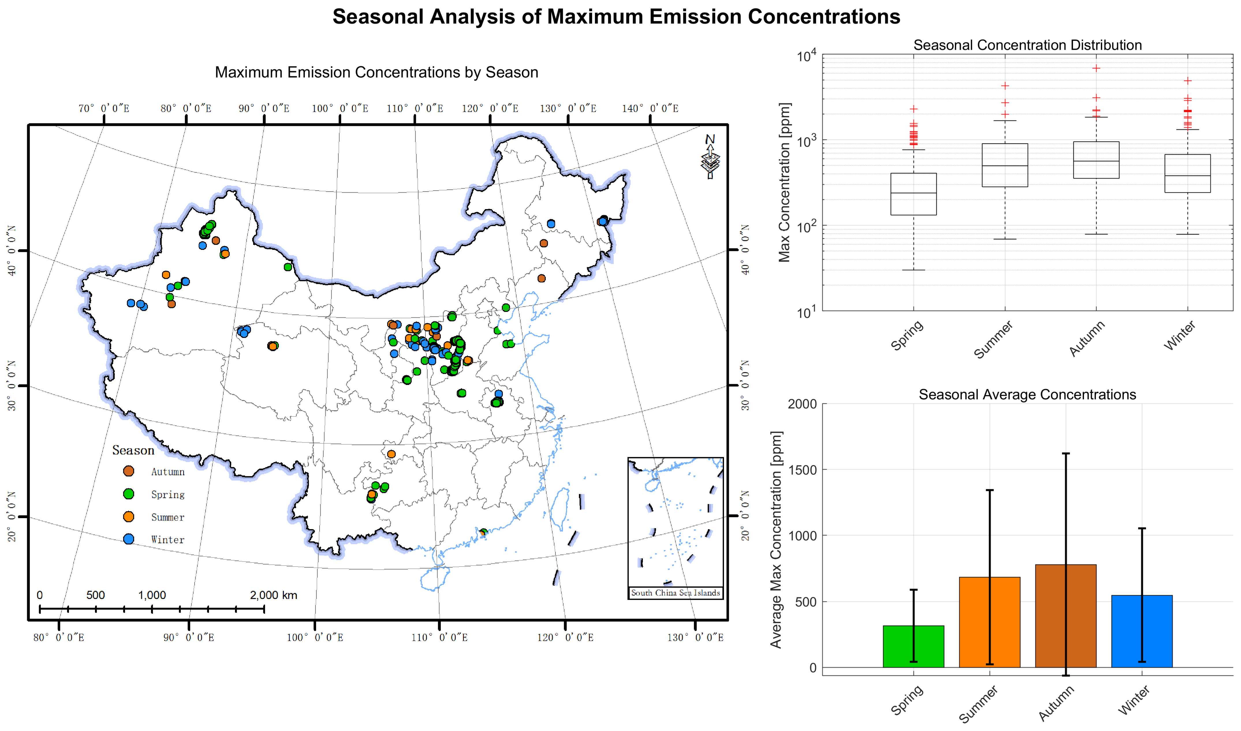
To illustrate the seasonal variability in simulated ground-level CH₄ concentrations, a seasonal analysis plot is presented in Figure 1. This plot displays the mean, standard deviation, and 95th percentile of maximum concentrations across four seasons (Spring, Summer, Autumn, Winter) for all Carbon Mapper observation sites during 2022–2025, highlighting both intra-seasonal fluctuations and inter-seasonal differences.

Figure 1 shows the seasonal distribution of simulated ground-level CH₄ concentrations, with Autumn exhibiting the highest mean maximum concentration (779.86 ppm) and the largest variability (standard deviation: 841.51 ppm), followed by Summer (mean: 684.14 ppm, std: 660.25 ppm), Winter (mean: 547.13 ppm, std: 506.14 ppm), and Spring (mean: 315.73 ppm, std: 274.38 ppm). The 95th percentile of concentrations in Autumn reaches 2187.25 ppm, substantially higher than that in Spring (877.99 ppm), indicating that high-concentration events are more frequent and intense in Autumn.

As visually evident from the boxplot morphology and outliers in Figure 1, the seasonal data mirror the heavy-tailed, log-normal behavior observed in the aggregate dataset. All seasons exhibit a distinct right-skewed pattern—with the mean concentration consistently higher than the median in each season—reflecting the prevalence of “super-emitter” phenomena that drive localized extreme values. This seasonal pattern not only confirms the highly localized nature of emissions but also reveals the modulation effect of meteorological conditions on concentration accumulation across different seasons.

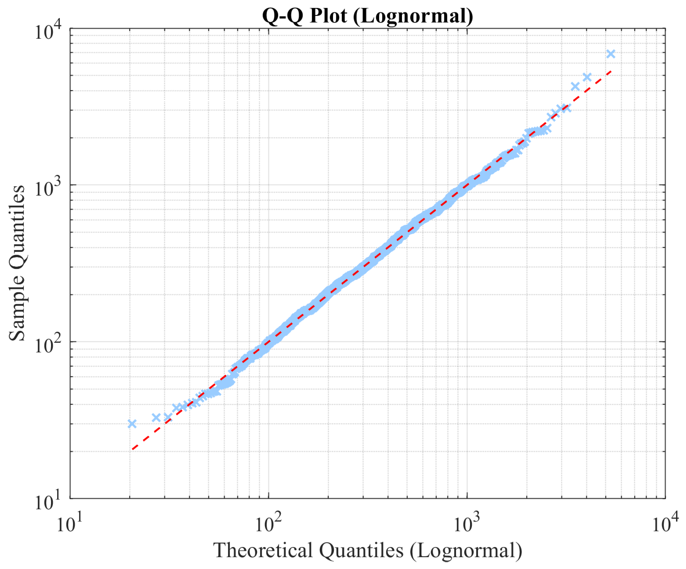
To verify whether the maximum ground-level concentration data conforms to a log-normal distribution, a Q-Q plot of the data was constructed, as shown in Figure 2.

The Q–Q plot in Figure 2 demonstrates that the distribution of simulated concentrations aligns closely with the log-normal distribution across the majority of the range (low to medium quantiles), as evidenced by the data points adhering to the red reference line. However, a distinct upward deviation is observed in the extreme upper quantiles. This deviation indicates that the actual high-concentration events are more intense than those predicted by the theoretical log-normal model. Such a characteristic confirms the presence of “heavy tail” in the dataset, implying that a small number of super-emitters exert a disproportionate influence on the regional emission pattern.

Based on the aforementioned overall analysis of the Gaussian model simulation results, we further explored the differential characteristics of high-emission events across different emission source types and geographical regions. For this purpose, all high-emission sites with simulated concentrations exceeding 1000 ppm were extracted. The statistics on the number of high-emission sites and average maximum concentration by sector are presented in

Table 3. Statistics on the Number of High-Emission Sites and Average Maximum Concentration by Sector.

Source Sector (IPCC)	Count	Mean Max Concentration (ppm)
Coal Mining (1B1a)	63	1547
Oil & Gas (1B2)	8	1647.6
Solid Waste (6A)	6	1931.1
Livestock (4B)	1	2185.5
Other	5	1818.1

, and by province in

Table 4. Statistics on the Number of High-Emission Sites and Average Maximum Concentration by Province.

Province	Count	Mean Max Concentration (ppm)
Shanxi	62	1583.9
Xinjiang Uygur Autonomous Region	8	1921.2
Shaanxi	4	1789.5
Qinghai	3	1790.1
Other	6	1100–1300

.

As presented in Table 3, the coal mining sector (IPCC code 1B1a) accounts for the largest number of high-emission sites, with a total of 63, underscoring its dominant contribution to methane super-emitters in China. Nevertheless, when considering the mean maximum concentration, sites associated with the solid waste treatment (6A) and oil and gas extraction (1B2) sectors, despite their smaller numbers, exhibit higher per-source intensities of 1931.1 ppm and 1647.6 ppm, respectively. This highlights their significant role in contributing to localized high-concentration exposure risks, which should not be overlooked in emission management strategies.

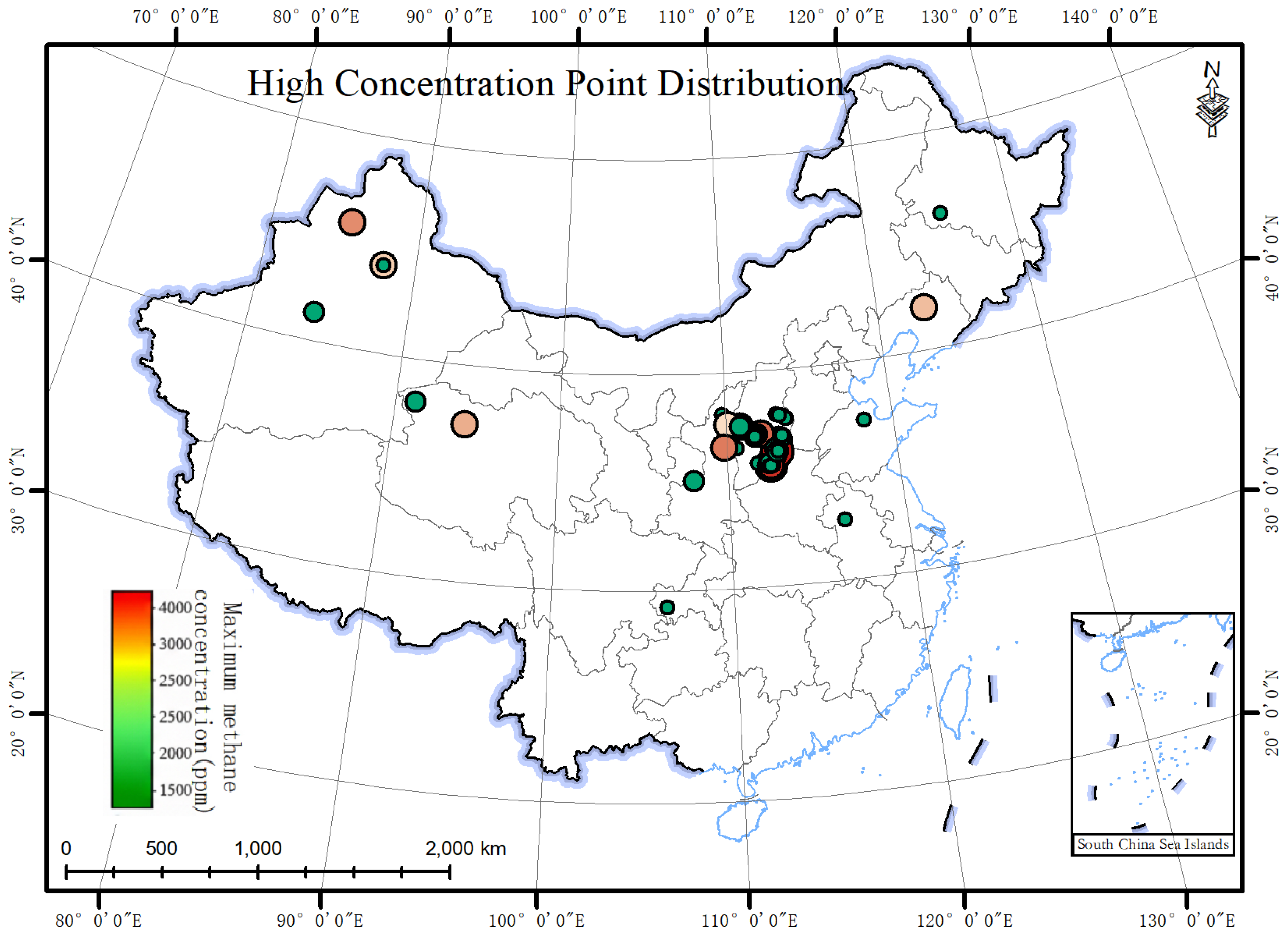
In terms of regional distribution, high-concentration sites are primarily clustered in traditional energy extraction regions such as Shanxi, Xinjiang, Shaanxi, and Qinghai, with Shanxi Province exhibiting the highest concentration, hosting 62 high-emission sites with a mean maximum concentration of 1583.9 ppm, indicating a pronounced regional aggregation. Although western regions such as Xinjiang and Qinghai have fewer sites, their mean concentrations are higher, suggesting that some sites may correspond to super-emission sources or occur under less favorable meteorological dispersion conditions. The detailed spatial distribution is presented in Table 4.

Figure 3 illustrates the spatial distribution of high-emission sites in mainland China with maximum simulated concentrations exceeding 1000 ppm during the 2022–2025 period. The figure indicates that these super-emitters are predominantly concentrated in energy-intensive regions of North and Northwest China, particularly in Shanxi, Xinjiang, Shaanxi, and Qinghai provinces, reflecting the central role of resource-based industries in regional methane pollution. In Shanxi, high-concentration sites are densely clustered in traditional coal mining areas such as Jinzhong, Lvliang, and Northern Shanxi, whereas sites in Xinjiang and Qinghai are more frequently associated with oil and gas production bases. This “sparse in the east, dense in the central and western regions” pattern further confirms that the high-value tail in the simulation results largely originates from industrial clusters, providing a spatial basis for developing emission control strategies that jointly consider both sectoral and geographic dimensions.

3.2. Sensitivity Analysis of Atmospheric Stability on Near-Surface Methane Concentrations

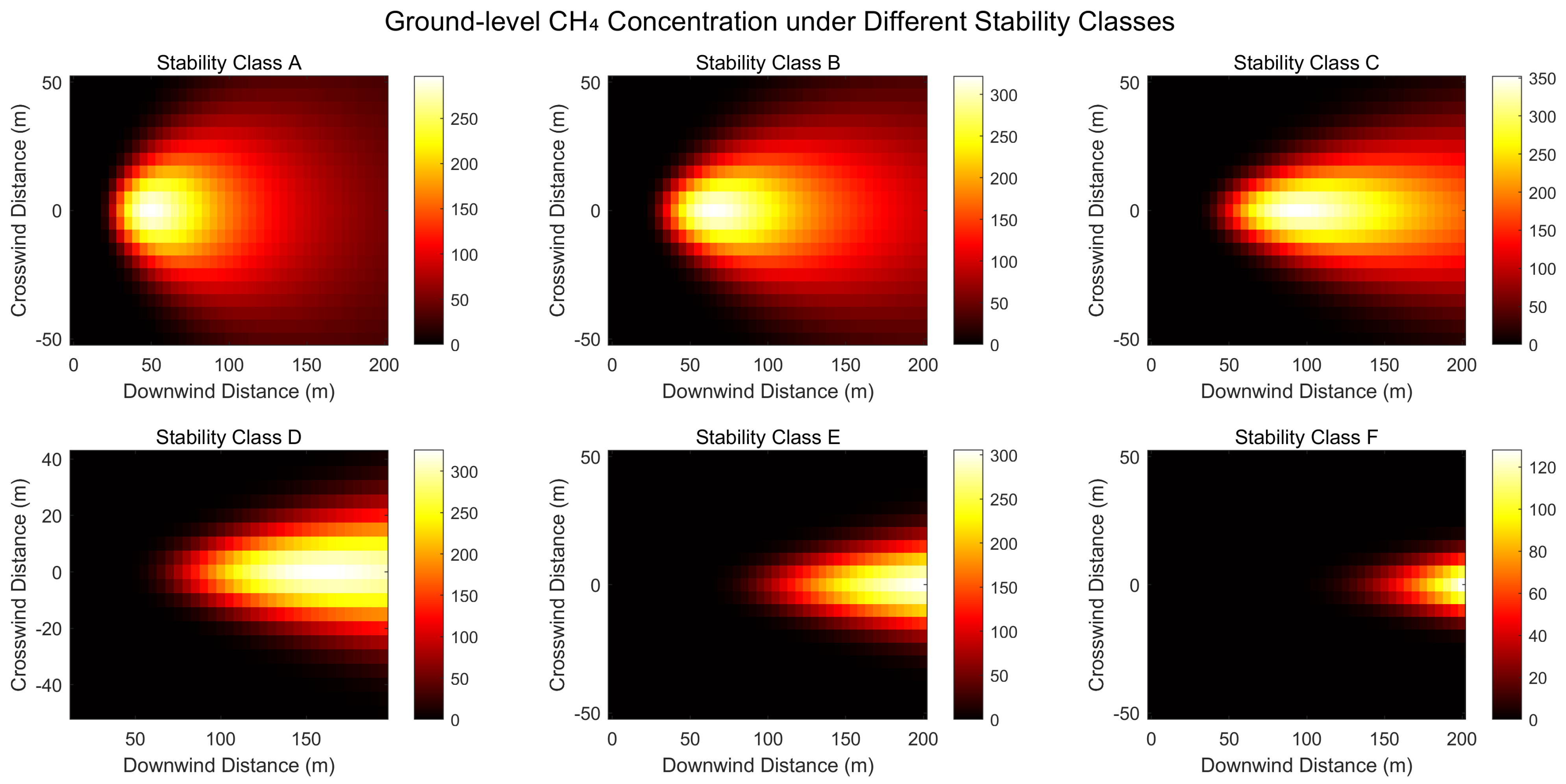
To investigate the impact of atmospheric stability on plume behavior—a fundamental mechanism governing plume spread and dispersion well-documented in meteorological literature [28,29]—this study simulated the concentration distribution under different stability classes: Class A (strongly unstable), Class B (unstable), Class C (weakly unstable), Class D (neutral), Class E (moderately stable), and Class F (stable).

To systematically compare the plume concentration distributions across these classes, Figure 4 is presented. To ensure comparability and isolate the effects of stability, these simulations were conducted using controlled parameter inputs: the emission rate (Q) was held constant at a representative value (1500 kg/h), and the wind speed (U) was fixed at 3 m/s. Under these conditions, variations in the concentration field are driven solely by the stability-dependent dispersion coefficients (${\sigma }_y,{\sigma }_z$), effectively illustrating the regulatory role of atmospheric turbulence on plume morphology.

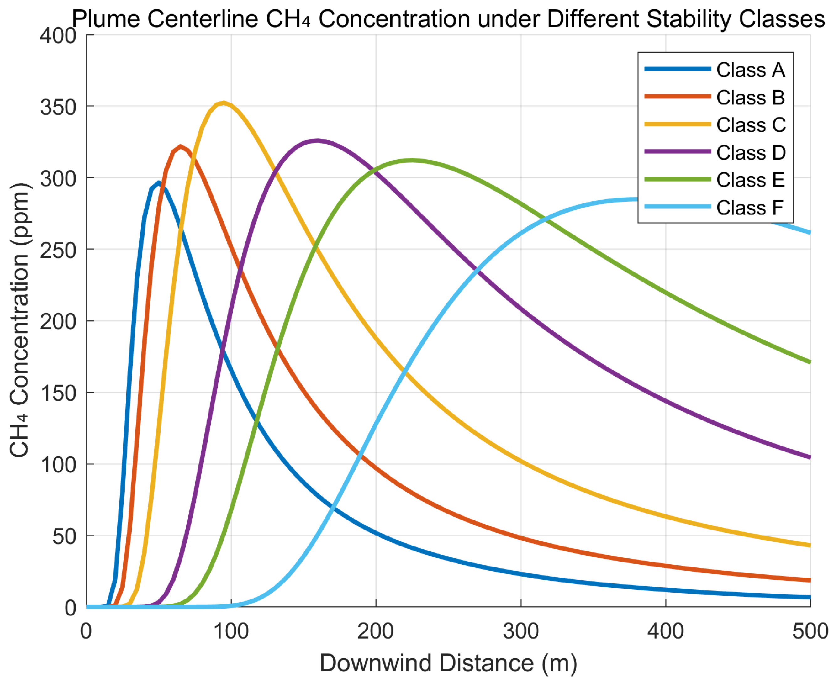
To show the distribution of plume centerline concentrations under different stability classes, Figure 5 is provided.

The simulation results under different stability classes further indicate that atmospheric stability exerts a significant influence on plume morphology and concentration distribution. The regulatory effects of varying atmospheric stability on plumes are manifested as follows: under unstable conditions (Classes A/B), vertical diffusion is enhanced, leading to a high degree of dispersion in the concentration field and relatively low centerline concentrations; in contrast, under stable or neutral conditions (Classes D–F), diffusion is restricted, and concentrations are highly concentrated in the near-to-medium downwind areas along the centerline, exhibiting a “thin and dense” characteristic.

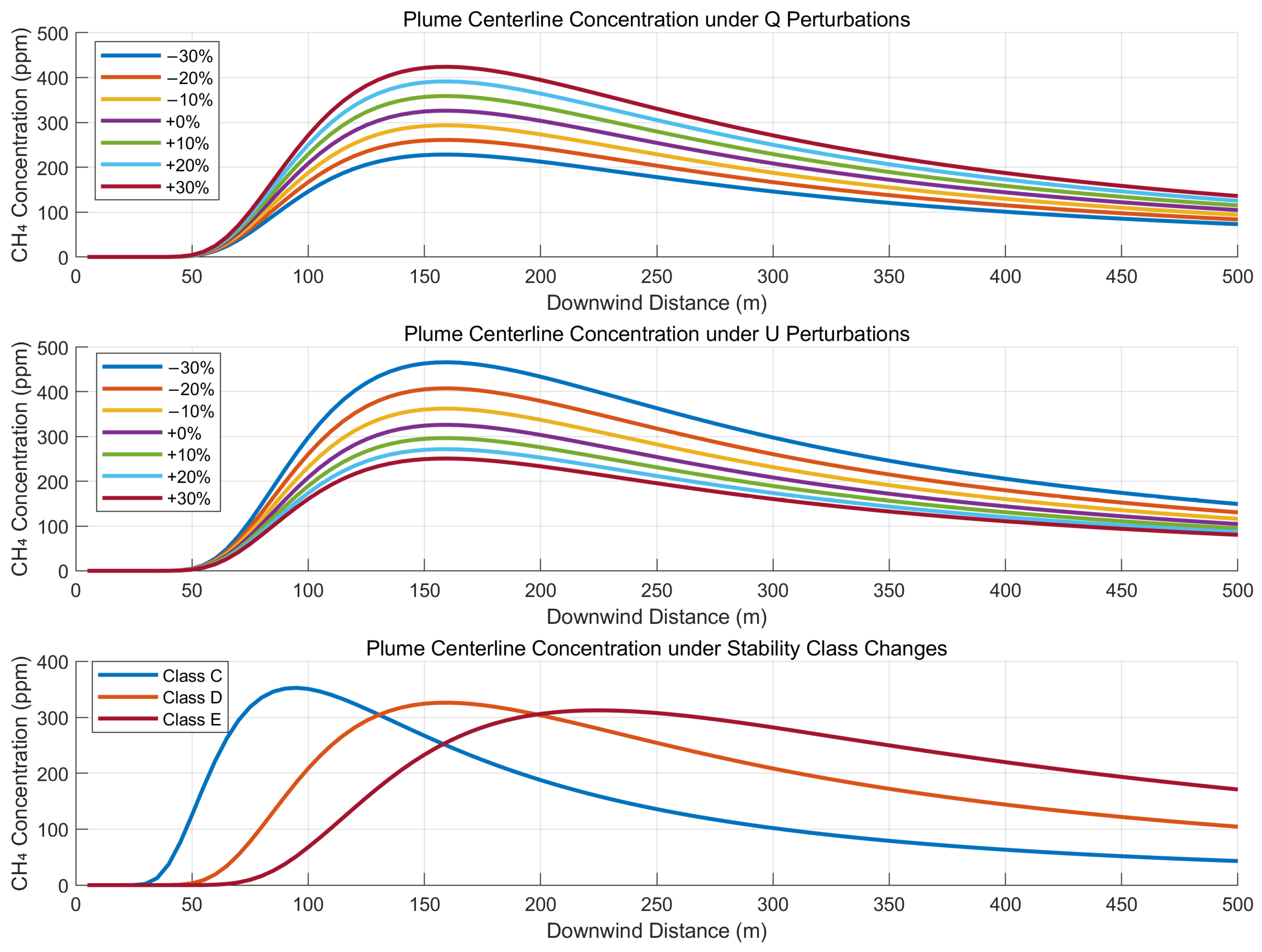
To evaluate the responsiveness of model output to key parameters, this study conducted perturbation simulations of emission rate (Q) and wind speed (U) with variations of ±10%, ±20%, and ±30%, respectively. These perturbations were implemented across different stability classes, and the rate of change in maximum concentration was analyzed.

To illustrate the sensitivity analysis of parameter perturbations (emission rate, wind speed, stability) on plume centerline concentration, Figure 6 is presented.

Figure 6 shows the variation in ground-level maximum concentration along the plume centerline under ±10% to ±30% perturbations of emission rate, wind speed, and atmospheric stability class. The three parameters exhibit distinct response patterns.

For emission rate, concentrations increase nearly linearly, with a ±30% change in emissions producing an almost proportional change in maximum concentration, highlighting the direct linear control of source strength.

Wind speed perturbations yield an inverse and nonlinear effect: higher wind speeds reduce concentrations, with stronger sensitivity at low wind speeds. A ±30% perturbation alters the maximum concentration by more than ±25%, with decreases exceeding increases, underscoring the strong dilution role of wind.

Stability class produces stepwise rather than continuous changes, reflecting its discrete nature. From class C (less stable) to class E (more stable), concentrations rise and then level off, with E-class peaks about 1.3 times higher than C-class, indicating greater accumulation risks under stable conditions.

In summary, the sensitivity analysis corroborates the theoretical behavior deduced from the analytical Gaussian model: it confirms the linear amplification driven by emission rate (verified via the perturbation plots in Figure 6), the inverse nonlinear dilution caused by wind speed, and the discrete structural modulation imposed by stability classes. These findings establish a physical basis for the subsequent uncertainty quantification and error propagation modeling.

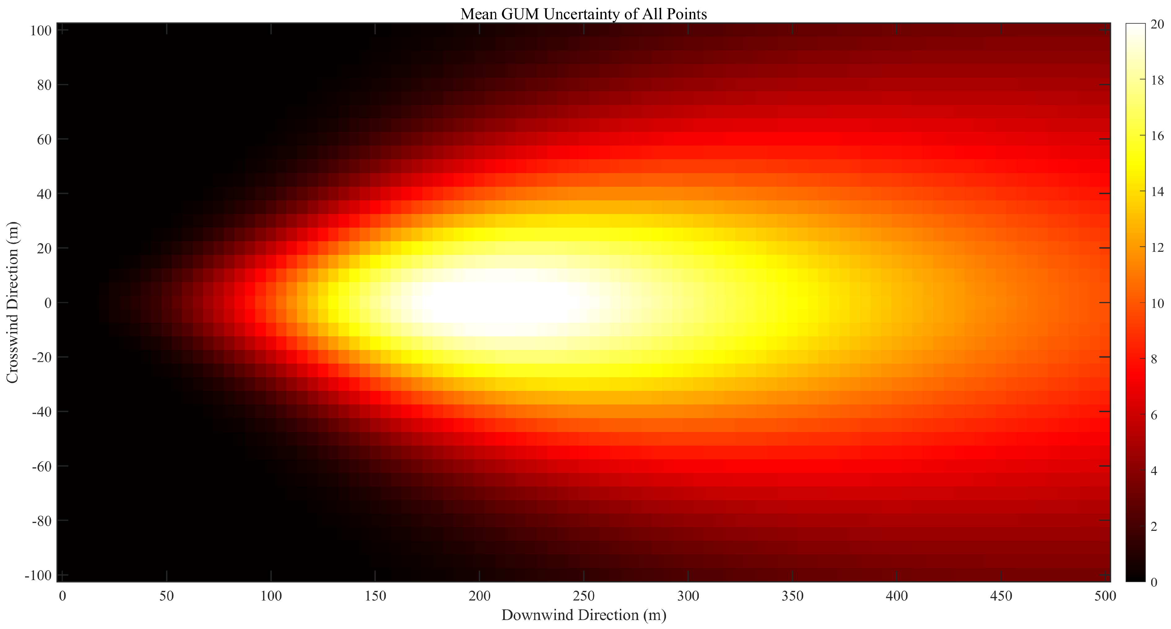
To further characterize the spatial distribution of uncertainties across all emission points under typical atmospheric conditions, this study employed the Monte Carlo method to perform joint simulations for all Carbon Mapper emission points during 2022–2025. The resulting two-dimensional uncertainty fields were extracted within a 500 m downwind and ±100 m crosswind range (Figure 7).This map represents the ensemble-averaged state derived from the full range of historical meteorological conditions (encompassing stability classes A–F) observed during the study period. The map is constructed on a 5 m resolution grid, where the color intensity represents the standard deviation of the simulated concentrations, reflecting the magnitude and spatial distribution of the output uncertainty in response to perturbations in input parameters such as emission rate, wind speed, and atmospheric stability.

It can be observed that the maximum uncertainty is typically concentrated within the range of 150–300 m near the downwind centerline of the source, presenting a typical pattern of “high in the center and low at the boundaries”. This spatial pattern implies that measurements taken within this high-uncertainty zone (150–300 m) are subject to significant model error. Consequently, monitoring campaigns should either avoid these high-gradient regions or assign lower weights to observations from these distances to minimize errors in inverted emission rates.

To contextualize our findings within a global framework,

Table 5. Comparison of statistical characteristics and uncertainty levels between the forward simulations in this study and regional inversion studies.

Region/Study	Methodology	Heavy-Tail Characteristic	Mean Intensity	Uncertainty Level c
China (This Study)	Forward Simulation	Heavy-tailed a	High	∼20–30% b
Four Corners, USA [27]	Airborne Retrieval	Top 10% contrib. 49–66%	Moderate	N/A
Permian Basin, USA [30]	Airborne Retrieval	Top 20% contrib. 60%	Very High	N/A
Global Controlled Test [16]	Satellite Inversion	N/A	Varied	∼30% (1$\sigma$)

^a Calculated based on the cumulative distribution of simulated near-surface concentrations. ^b Represents the ensemble standard deviation (statistical dispersion) derived from forward Monte Carlo simulations. ^c Notation difference: Approximate values (∼) denote model output dispersion (standard deviation), whereas other values denote retrieval error budgets relative to ground truth.

presents a comparison between the characteristics of high-emission point sources in China and those in major U.S. basins. Although this study employs forward dispersion modeling rather than emission inversion, the results demonstrate a fundamental consistency in physical patterns. The simulated near-surface concentrations exhibit a distinct heavy-tailed structure. For instance, Frankenberg et al. reported that the top 10% of emitters contribute 49–66% of the total flux in the Four Corners region [27], and Cusworth et al. found that the top 20% of sources constitute 60% of emissions in the Permian Basin [30]. This confirms that the dominance of super-emitters is a universal feature that propagates from emission sources to the concentration field, regardless of the modeling direction. Furthermore, the uncertainty range derived from our forward Monte Carlo analysis (∼20–30%) is comparable to the error budgets reported in retrieval studies. This correspondence may suggest that the parametric sensitivities quantified in our forward model (particularly to wind speed and stability) constitute the primary physical baseline for the errors observed in satellite-based inversions.

3.3. Discussion

Gaussian plume simulations based on Carbon Mapper data reveal the fundamental dispersion characteristics of high-emission point sources. Our simulated mean concentration of 475.9 ppm underscores the intense local environmental impact of these sites. The observed heavy-tailed distribution aligns with findings by Frankenberg et al. [27] in the U.S. and studies in the Permian Basin [17,31], confirming the recurrence of skewed emission patterns across diverse industrial contexts. This consistency with established literature serves as a basic verification of our model’s performance in the absence of in-situ ground validation.

The sensitivity analysis results are grounded in physical mechanisms. The linear response to emission rate variations confirms the direct link between source strength and concentration [9]. More notably, the inverse nonlinear response to wind speed arises because wind speed (U) determines the air volume available for dilution per unit time. As U approaches zero, the dilution volume decreases asymptotically, causing sharp concentration spikes. This corroborates findings that low wind speeds are a dominant source of retrieval uncertainty [6], as unfavorable meteorological conditions can disproportionately amplify emission impacts. Similarly, the stepwise impact of atmospheric stability reflects the suppression of vertical turbulent mixing. Under stable conditions (Class E), thermal stratification restricts vertical eddy diffusion, confining the plume to a shallow layer and increasing ground-level accumulation [25]. This explains why stable conditions yield peak concentrations ∼1.3 times higher than unstable ones, consistent with recent vertical dispersion studies [15].

Our uncertainty analysis exposes error distributions masked by deterministic approaches. Unlike single-state simulations [22], our Monte Carlo results exhibit a heavy-tailed uncertainty profile. This implies that regional inversions relying solely on mean wind speeds [32] may underestimate risks from super-emitters under non-steady conditions. Furthermore, extending beyond coal-focused studies [20], we show that the oil & gas and solid waste sectors exhibit distinct sensitivities to stability parameters, necessitating the development of sector-specific uncertainty protocols.

Regionally, the agglomeration of high concentrations in Shanxi and Xinjiang highlights the environmental footprint of energy-intensive industries. While coal mining dominates in site count, the oil & gas and solid waste sectors show higher per-source intensities. This pattern necessitates rigorous validation, as recent satellite-based mappings have revealed significant discrepancies in sectoral emission attributions across Asia, identifying missing or underestimated sources in standard inventories [33]. This underscores the need for region-specific emission inventories that account for local industrial structures.

Limitations

This study has limitations. First, the lack of ground-based validation was partially remedied by strictly utilizing validated Level-4B Carbon Mapper products and literature-based consistency checks. Second, the coarse resolution of ERA5 ($0.25°$, ≈30 km) limits the resolution of sub-grid topographic effects and micro-scale wind heterogeneity, potentially introducing systematic biases in plume trajectories within complex terrain.

Additionally, the Gaussian steady-state assumption simplifies the temporal variability inherent in anthropogenic sectors (e.g., coal and waste). However, by employing “persistence-adjusted” emission rates from Carbon Mapper, this study targets “chronic” super-emitters rather than transient venting events. While this temporal aggregation may smooth out extreme instantaneous peaks—potentially underestimating acute short-term exposure—it yields representative hourly averages during active episodes, effectively capturing the baseline footprint of persistent sources in line with regulatory goals. Future work should incorporate 3D terrain effects and atmospheric chemistry to refine long-term assessments.Furthermore, future improvements in emission inventory accuracy will likely benefit from rigorous validation campaigns, such as recent controlled release experiments designed to assess the performance of next-generation imaging spectrometers like MethaneAIR [34,35].

4. Conclusions

Using satellite-derived methane emission rates from Carbon Mapper as prescribed inputs and ERA5 reanalysis meteorological data, this study quantified how input parameter uncertainties propagate through forward Gaussian plume simulations of near-surface methane concentrations using a Monte Carlo framework. The numerical results show that simulated concentrations exhibit a heavy-tailed distribution (mean 475.88 ppm, 95th percentile 1292.12 ppm), highlighting the dominant role of super-emitters. Sectoral and regional analyses identify coal mining (1B1a) and the Shanxi region as major contributors to high-concentration occurrences, while the solid waste and oil & gas sectors display higher per-source emission intensities. Sensitivity analysis indicates an approximately linear concentration response to emission rate perturbations, contrasted with inverse nonlinear and discrete structural effects associated with wind speed and atmospheric stability, respectively. Monte Carlo simulations further identify the 150–300 m downwind range as the region of maximum output uncertainty, suggesting that forward-model– observation comparisons should avoid this high-gradient zone to reduce mismatch errors. Overall, these findings provide a quantitative basis for prioritizing uncertainty reduction in plume-based concentration modeling and offer valuable knowledge to support, rather than perform, satellite-based emission inversions and region- and sector-specific mitigation strategies.

References

1. Saunois, M.; Stavert, A.R.; Poulter, B.; Bousquet, P.; Canadell, J.G.; Jackson, R.B.; Raymond, P.A.; Dlugokencky, E.J.; Houweling, S.; Patra, P.K.; et al. The global methane budget 2000–2017. Earth Syst. Sci. Data 2020, 12, 1561–1623. [Google Scholar] [CrossRef] [Scilit]
2. Nisbet, E.G.; Fisher, R.E.; Lowry, D.; France, J.L.; Allen, G.; Bakkaloglu, S.; Broderick, T.J.; Cain, M.; Coleman, M.; Fernandez, J.; et al. Methane mitigation: Methods to reduce emissions, on the path to the Paris agreement. Rev. Geophys. 2020, 58, e2019RG000675. [Google Scholar] [CrossRef] [Scilit]
3. United Nations Environment Programme and Climate and Clean Air Coalition. Global Methane Assessment: Benefits and Costs of Mitigating Methane Emissions; United Nations Environment Programme and Climate and Clean Air Coalitio: Nairobi, Kenya, 2021. [Google Scholar]
4. Ministry of Ecology and Environment of the People’s Republic of China. Methane Emission Control Action Plan. Beijing, China, 7 November 2023; Notice No. [2023] 67. Available online: https://www.gov.cn/zhengce/zhengceku/202311/content_6914109.htm (accessed on 12 December 2024).
5. Collins, W.; Orbach, R.; Bailey, M.; Biraud, S.; Coddington, I.; DiCarlo, D.; Peischl, J.; Radhakrishnan, A.; Schimel, D. Monitoring methane emissions from oil and gas operations. PRX Energy 2022, 1, 017001. [Google Scholar] [CrossRef] [Scilit]
6. Jacob, D.J.; Turner, A.J.; Maasakkers, J.D.; Sheng, J.; Sun, K.; Liu, X.; Chance, K.; Aben, I.; McKeever, J.; Frankenberg, C. Satellite observations of atmospheric methane and their value for quantifying methane emissions. Atmos. Chem. Phys. 2016, 16, 14371–14396. [Google Scholar] [CrossRef] [Scilit]
7. Lu, X.; Jacob, D.J.; Zhang, Y.; Maasakkers, J.D.; Sulprizio, M.P.; Shen, L.; Qu, Z.; Scarpelli, T.R.; Nesser, H.; Yantosca, R.M.; et al. Global methane budget and trend, 2010–2017. Atmos. Chem. Phys. 2021, 21, 4637–4657. [Google Scholar] [CrossRef] [Scilit]
8. Bruno, J.H.; Jervis, D.; Varon, D.J.; Jacob, D.J. U-Plume: Automated algorithm for plume detection and source quantification by satellite point-source imagers. Atmos. Meas. Tech. 2024, 17, 2625–2636. [Google Scholar] [CrossRef] [Scilit]
9. Varon, D.J.; Jacob, D.J.; McKeever, J.; Jervis, D.; Durak, B.O.A.; Xia, Y.; Huang, Y. Quantifying methane point sources from fine-scale satellite observations of atmospheric methane plumes. Atmos. Meas. Tech. 2018, 11, 5673–5686. [Google Scholar] [CrossRef] [Scilit]
10. Turner, A.J.; Frankenberg, C.; Kort, E.A. Interpreting contemporary trends in atmospheric methane. Proc. Natl. Acad. Sci. USA 2019, 116, 2805–2813. [Google Scholar] [CrossRef] [Scilit]
11. Schwietzke, S.; Pétron, G.; Conley, S.; Pickering, C.; Mielke-Maday, I.; Dlugokencky, E.J.; Tans, P.P.; Vaughn, T.; Bell, C.; Zimmerle, D.; et al. Improved mechanistic understanding of natural gas methane emissions. Environ. Sci. Technol. 2017, 51, 7286–7294. [Google Scholar] [CrossRef] [Scilit]
12. Plant, G.; Kort, E.A.; Brandt, A.R.; Chen, Y.; Fordice, G.; Gorchov Negron, A.M.; Schwietzke, S.; Smith, M.; Zavala-Araiza, D. Inefficient and unlit natural gas flares both emit large quantities of methane. Science 2022, 377, 1566–1571. [Google Scholar] [CrossRef] [Scilit]
13. Saltelli, A.; Aleksankina, K.; Becker, W.; Fennell, P.; Ferretti, F.; Holst, N.; Li, S.; Wu, Q. Why so many published sensitivity analyses are false. Environ. Model. Softw. 2019, 114, 29–39. [Google Scholar] [CrossRef] [Scilit]
14. Caulton, D.R.; Shepson, P.B.; Santoro, R.L.; Sparks, J.P.; Howarth, R.W.; Ingraffea, A.R.; Cambaliza, M.O.; Sweeney, C.; Karion, A.; Davis, K.J.; et al. Toward a better understanding and quantification of methane emissions from shale gas development. Proc. Natl. Acad. Sci. USA 2014, 111, 6237–6242. [Google Scholar] [CrossRef] [Scilit]
15. Mohammadi, M.; Mohammadi, M.; Moezzi, S.M.M. Air pollution meteorology and dispersion. In Air Pollution, Air Quality, and Climate Change; Elsevier: Amsterdam, The Netherlands, 2025; pp. 51–82. [Google Scholar]
16. Sherwin, E.D.; El Abbadi, S.H.; Burdeau, P.M.; Zhang, Z.; Chen, Z.; Rutherford, J.S.; Chen, Y.; Brandt, A.R. Single-blind test of nine methane-sensing satellite systems from three continents. Atmos. Meas. Tech. 2024, 17, 765–782. [Google Scholar] [CrossRef] [Scilit]
17. Zavala-Araiza, D.; Lyon, D.R.; Alvarez, R.A.; Davis, K.J.; Harriss, R.; Herndon, S.C.; Karion, A.; Kort, E.A.; Lamb, B.K.; Lan, X.; et al. Reconciling divergent estimates of oil and gas methane emissions. Proc. Natl. Acad. Sci. USA 2015, 112, 15597–15602. [Google Scholar] [CrossRef] [Scilit]
18. Duren, R.M.; Thorpe, A.K.; Foster, K.T.; Rafiq, T.; Hopkins, F.M.; Yadav, V.; Bue, B.D.; Thompson, D.R.; Conley, S.; Colombi, N.K.; et al. California’s methane super-emitters. Nature 2019, 575, 180–184. [Google Scholar] [CrossRef] [Scilit]
19. Tu, Q.; Hase, F.; Qin, K.; Cohen, J.B.; Khosrawi, F.; Zou, X.; Schneider, M.; Lu, F. Quantifying CH4 emissions from coal mine aggregation areas in Shanxi. Atmos. Chem. Phys. 2024, 24, 4875–4894. [Google Scholar] [CrossRef] [Scilit]
20. He, Z.; Gao, L.; Liang, M.; Zeng, Z.-C. A survey of methane point source emissions from coal mines in Shanxi province of China using AHSI on board Gaofen-5B. Atmos. Meas. Tech. 2024, 17, 2937–2956. [Google Scholar] [CrossRef] [Scilit]
21. Li, X.; Cheng, T.; Zhu, H.; Ye, X.; Fan, D.; Tang, T.; Tong, H.; Yin, S.; Xiong, J. High-resolution satellite reveals methane emissions from China’s coal mines. Remote Sens. 2025, 17, 220. [Google Scholar] [CrossRef] [Scilit]
22. Zhang, Y. Quantitative Study on Methane Emission in Liaoning Province Based on Gaussian Plume Model. Front. Environ. Res. 2025, 3, 67–71. [Google Scholar] [CrossRef] [Scilit]
23. Cotlier, G.I.; de Miranda, V.F.V.V.; Jimenez, J.C. Characterization and Quantification of Methane Emission Plumes and Super-Emitter Detection Across North-Central Brazil Using Hyperspectral Satellite Data. Remote Sens. 2025, 17, 3973. [Google Scholar] [CrossRef] [Scilit]
24. Carbon Mapper. Carbon Mapper Data Portal. Available online: https://carbonmapper.org/data/ (accessed on 12 December 2024).
25. Turner, D.B. Workbook of Atmospheric Dispersion Estimates: An Introduction to Dispersion Modeling, 2nd ed.; CRC Press: Boca Raton, FL, USA, 1994. [Google Scholar]
26. Seinfeld, J.H.; Pandis, S.N. Atmospheric Chemistry and Physics: From Air Pollution to Climate Change, 3rd ed.; John Wiley & Sons: Hoboken, NJ, USA, 2016. [Google Scholar]
27. Frankenberg, C.; Thorpe, A.K.; Thompson, D.R.; Hulley, G.; Kort, E.A.; Vance, N.; Borchardt, J.; Krings, T.; Gerilowski, K.; Sweeney, C.; et al. Airborne methane remote measurements reveal heavy-tail flux distribution in Four Corners region. Proc. Natl. Acad. Sci. USA 2016, 113, 9734–9739. [Google Scholar] [CrossRef] [Scilit] [PubMed]
28. Venkatram, A.; Isakov, V.; Yuan, J.; llen, D.T.; Barkley, Z.R.; Brandt, A.R.; Davis, K.J.; Herndon, S.C.; Jacob, D.J.; Karion, A.; et al. Relating plume spread to meteorology in urban areas. Atmos. Environ. 2005, 39, 371–380. [Google Scholar] [CrossRef] [Scilit]
29. Gifford, F.A. Use of routine meteorological observations for estimating atmospheric dispersion. Nucl. Saf. 1961, 2, 47–57. [Google Scholar]
30. Cusworth, D.H.; Duren, R.M.; Thorpe, A.K.; Olson-Duvall, W.; Heckler, J.; Chapman, J.W.; Eastwood, M.L.; Helmlinger, M.C.; Green, R.O.; Asner, G.P.; et al. Intermittency of Large Methane Emitters in the Permian Basin. Environ. Sci. Technol. Lett. 2021, 8, 567–573. [Google Scholar] [CrossRef] [Scilit]
31. Alvarez, R.A.; Zavala-Araiza, D.; Lyon, D.R.; Allen, D.T.; Barkley, Z.R.; Brandt, A.R.; Davis, K.J.; Herndon, S.C.; Jacob, D.J.; Karion, A.; et al. Assessment of methane emissions from the US oil and gas supply chain. Science 2018, 361, 186–188. [Google Scholar] [CrossRef] [Scilit]
32. Feng, S.; Jiang, F.; Zhang, Y.; Chen, H.; Zhuang, H.; Wang, S.; Bai, S.; Wang, H.; Ju, W. High-resolution regional inversion reveals overestimation of anthropogenic methane emissions in China. Atmos. Chem. Phys. 2025, 25, 15121–15143. [Google Scholar] [CrossRef] [Scilit]
33. Yu, X.; Millet, D.B.; Henze, D.K.; Turner, A.J.; Delgado, A.L.; Bloom, A.A.; Sheng, J. A high-resolution satellite-based map of global methane emissions reveals missing wetland, fossil fuel, and monsoon sources. Atmos. Chem. Phys. 2023, 23, 3325–3346. [Google Scholar] [CrossRef] [Scilit]
34. Chulakadabba, A.; Sargent, M.; Lauvaux, T.; Benmergui, J.S.; Franklin, J.E.; Chan Miller, C.; Wilzewski, J.S.; Roche, S.; Conway, E.; Souri, A.H.; et al. Methane point source quantification using MethaneAIR: A new airborne imaging spectrometer. Atmos. Meas. Tech. 2023, 16, 5771–5785. [Google Scholar] [CrossRef] [Scilit]
35. Guanter, L.; Warren, J.; Omara, M.; Chulakadabba, A.; Roger, J.; Sargent, M.; Franklin, J.E.; Wofsy, S.C.; Gautam, R. Detection and quantification of methane plumes with the MethaneAIR airborne spectrometer. Atmos. Meas. Tech. 2025, 18, 3857–3872. [Google Scholar] [CrossRef]
Figure 1. Seasonal box-plot statistics of simulated ground-level methane (CH4) concentrations. The horizontal axis represents the four seasons, and the vertical axis shows the maximum plume centerline concentration (ppm) on a logarithmic scale. Boxes denote the interquartile range (IQR) with the median indicated by the central line, while whiskers extend to 1.5 times the IQR. Red crosses indicate statistical outliers, representing potential super-emitter events.
Environments 13 00062 g001
Figure 2. Q–Q plot of maximum simulated ground-level CH4 concentrations against a theoretical log-normal distribution. Both axes represent concentrations in ppm on a logarithmic scale. The blue crosses denote the sample quantiles of the simulated concentration data, and the red dashed line represents the theoretical reference line for a standard log-normal distribution. While the bulk of the data follows a linear log-normal trend, the upward divergence in the upper tail reveals the presence of extreme concentrations that exceed theoretical expectations.
Environments 13 00062 g002
Figure 3. Spatial distribution of high-emission methane point sources in China (August 2022–June 2025). Each point represents an individual emission site, and the color scale indicates the maximum near-surface concentration (ppm) simulated for that specific location during the entire study period. Note that only super-emitters with peak concentrations exceeding 1000 ppm are displayed.
Environments 13 00062 g003
Figure 4. Comparison of Plume Concentration Distributions Under Different Atmospheric Stability Classes.
Environments 13 00062 g004
Figure 5. Distribution of Plume Centerline Concentrations Under Different Stability Classes.
Environments 13 00062 g005
Figure 6. Sensitivity Analysis Plot of Parameter Perturbations (Emission Rate, Wind Speed, Stability) on Plume Centerline Concentration.
Environments 13 00062 g006
Figure 7. Spatial Distribution Map of Methane Concentration Uncertainty Mean Under Monte Carlo Simulation.
Environments 13 00062 g007