Stream Community Metabolism and Dissolved-Oxygen Dynamics: Where Did the Oxygen Come From?

Abstract

Stream metabolism is traditionally defined as the combined metabolism of all aerobic organisms in a stream. Its component processes of oxygenic photosynthesis and aerobic respiration create and consume dissolved oxygen (DO) and therefore can be measured using time series of DO concentration, solar radiation, and water temperature, in conjunction with a model of DO dynamics that includes photosynthesis, respiration, and oxygen exchange with the atmosphere. A complication is that stream communities typically exhibit pronounced longitudinal heterogeneity in habitat type (e.g., shaded versus unshaded reaches) and species composition and abundance. The influence of a given stream reach and associated community on DO concentration propagates downstream with the current, gradually being replaced, over a transition zone, by the influence of the next downstream reach. Knowing the approximate length of this transition zone is important when estimating stream metabolism with one-station DO monitoring, since it indicates which stream reach and associated community the metabolism estimates apply to. We propose new methods for estimating the transition-zone length and for estimating the proportions of DO at a given location in a stream reach that entered the reach from upstream, from photosynthesis within the reach, and from atmospheric uptake within the reach. We also propose methods for estimating the residence-time distribution of DO present at a given stream location, and the corresponding distribution of upstream distances at which the DO entered the stream. Both distributions are approximately exponential. Thus, habitat immediately upstream of the sonde has the greatest influence on metabolism estimates with one-station monitoring, and it is therefore important to place the sonde so this habitat is representative of the study reach.

1. Introduction

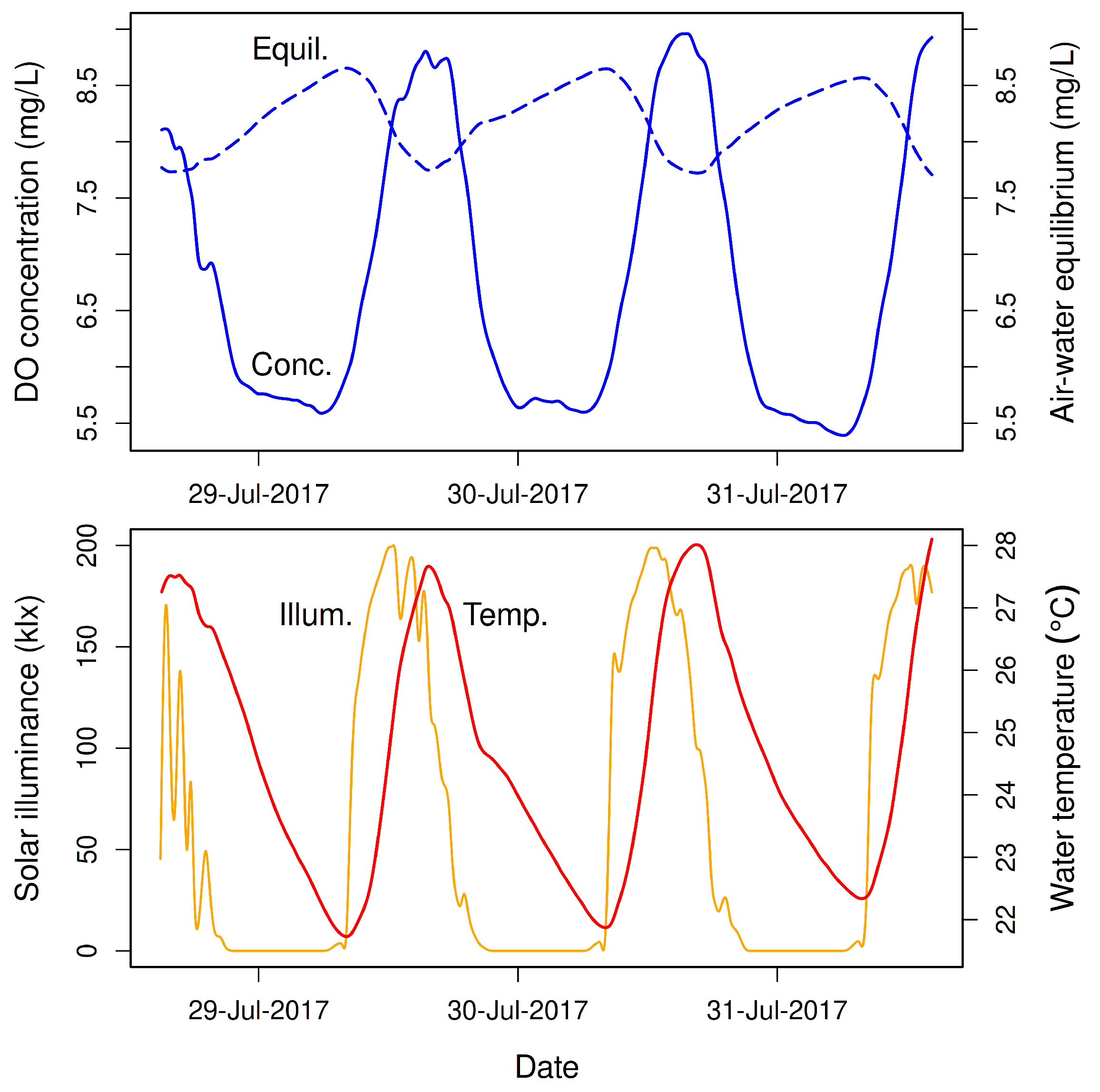
One of the most striking and predictable phenomena in healthy streams is the daily cycle of dissolved oxygen (DO) concentration that occurs during warm months of the year (Figure 1). This cycle is caused mainly by the combined metabolism of aerobic bacteria, eukaryotic algae, and submersed aquatic macrophytes. During daytime, oxygenic photosynthesis by photoautotrophs produces oxygen at a higher rate than it is consumed by aerobic respiration of photoautotrophs and heterotrophs (Figure 2). The DO concentration in the stream therefore increases sharply, often exceeding the gas-exchange equilibrium (“saturation”). During nightime, aerobic respiration by photoautotrophs and heterotrophs in the absence of photosynthesis causes a rapid decline in DO concentration, driving it well below the gas-exchange equilibrium. And so, as Odum and Hoskin [1] put it, streams “like great creatures breathe in and out” over each diel cycle.

The pronounced diel cycle of DO concentration in a stream, and the associated cycle of solar radiation that drives it, are the basis for a common method of estimating the rates of oxygen production and consumption by stream communities. This method employs times series of DO concentration, water temperature, and solar radiation, along with a process-based model of DO dynamics, to estimate rates of oxygenic photosynthesis and aerobic respiration. These rates are the main components of stream metabolism.

Various difficulties in the estimation process are created by the facts that stream water is continually flowing, and stream habitat and community structure typically exhibit marked longitudinal heterogeneity. In particular, these stream properties complicate the process of determining which stream reach and associated community a measured metabolic rate applies to. As flowing water enters a given stream reach, its DO concentration mainly reflects habitat and community structure upstream of the focal reach. As the water flows through the focal reach, its DO concentration changes and approaches a value characteristic of habitat and community structure in the focal reach. Thus, there is a transition zone in the initial portion of the focal reach, within which the DO concentration changes from being characteristic of the upstream reach to being characteristic of the focal reach. In order to obtain metabolism estimates that reflect the habitat and community structure of the focal reach, it is necessary to know the approximate length of this transition zone and to base the estimates on time series of DO concentration, solar radiation, and other predictor variables acquired downstream of the transition zone but still within the focal reach. A simple traditional estimate of transition-zone length has been widely employed by stream ecologists since the early 2000s (see Section 3), but we will argue that it fails to account for most of the key processes responsible for changes in DO concentration within the transition zone and therefore is inadequate.

The main goal of the present paper is to propose a new practical estimate of the length of the DO transition zone. In order to achieve this goal, it is necessary to extend the classical model of stream DO dynamics in several ways. The problem we address is of fundamental importance in stream ecology, but some of the empirical and theoretical background information necessary for understanding the problem and the approaches we will use to solve it is sufficiently specialized that many readers may be unfamiliar with it. Therefore, to make our paper accessible to as wide an audience as possible, we include a significant amount of background information that is necessary for understanding the model extensions we propose and their biological rationale.

The paper is organized as follows. Section 2 presents background empirical information on stream metabolism that is required for understanding the remainder of the paper; it can be skipped or skimmed by readers who are already familiar with this information. Section 3 presents the traditional estimate of DO transition-zone length. Section 4 presents an intuitive argument that reveals the main processes responsible for the changes in DO concentration that occur after water flows into a focal stream reach, only one of which is accounted for by the traditional estimate of transition-zone length. Section 5 outlines the classical model of stream DO dynamics and can be skipped or skimmed by readers who are already familiar with this model. Section 6 presents an extension of the classical model of stream DO dynamics, which distinguishes three types of DO in a focal stream reach (old DO that entered the stream upstream of the focal reach, new DO that entered the focal reach from the atmosphere, and new DO that was produced within the focal reach by photosynthesis), then uses the extended model to derive a new estimate of transition-zone length that accounts for all major processes responsible for changes in DO concentration within the transition zone. Section 7 assesses and compares the traditional and proposed estimates of transition-zone length with exact values computed using a more-realistic model of DO dynamics that includes an energy balance and transport model for water temperature, whose dynamics drive temporal variation in temperature-dependent process rates (photosynthesis, respiration, and exchange of oxygen with the atmosphere); this section can be skipped on a first reading. Section 8 shows how the traditional estimate of transition-zone length can be derived from the proposed new estimate, providing insight into conditions under which the two estimates will be similar; this section, too, can be skipped on a first reading. Section 9 compares the values of the traditional and proposed estimates of transition-zone length calculated using published data for several streams in eastern New York state (USA). Section 10 presents a second novel method of estimating the transition-zone length (based on the DO residence-time distribution instead of concentrations of the three types of old and new DO), which yields the same proposed estimate as the first method; it can be skipped on a first reading. Finally, Section 11 discusses the results, and Section 12 briefly summarizes the main takeaways from our study.

2. Background of the Problem

In this section, we summarize some necessary background information about stream metabolism, longitudinal heterogeneity in stream habitat, transition zones in water temperature and DO concentration that this heterogeneity creates, and the two main methods used for monitoring DO concentration and environmental predictor variables in studies of stream metabolism. Readers who are already familiar with this information may wish to skip or skim this section.

2.1. Stream Metabolism and Its Estimation

The aggregate metabolism of all aerobic organisms in a stream is commonly referred to as stream metabolism. The implied exclusion of anaerobic microbial metabolism (which is well known to occur in streams [3]) largely reflects the historical focus on DO concentration as a measure of water quality in rivers with high levels of anthropogenic organic pollution in the early to mid 1900s. For example, the Streeter-Phelps model [4], published in 1925, was developed in an effort to identify and characterize the main processes and rates underlying the pronounced decrease in DO concentration in the Ohio River (USA) immediately downstream from Pittsburgh (Pennsylvania) and Cincinnati (Ohio), and the gradual increase in concentration that occurred farther downstream. Based on a simple plug-flow model of stream flow to which rates of oxygen exchange with the atmosphere and DO consumption by aerobic microbial respiration were added, the model was able to adequately describe the longitudinal pattern of DO concentration downstream from each city. In the 1950s and later, photosythetic production of DO was added to the model by Odum [5] and others (e.g., [6,7,8,9,10]). Aquatic ecologists then began to use the expanded model for the opposite purpose of inferring rates of aerobic metabolism from observed DO concentrations instead of predicting DO concentrations from rates of aerobic metabolism and atmospheric exchange (e.g., [1,5,7,9,10,11]). Use of the expanded model by aquatic ecologists was often implicit, based on a verbal intuitive interpretation of water and DO transport that the plug-flow assumption makes possible.

The two main components of stream metabolism are oxygenic photosynthesis and aerobic respiration. Because it integrates over the entire aerobic community, stream metabolism is a measure of overall community function that is useful for comparing different streams, different reaches within a stream, or the same reaches at different times (e.g., [12,13,14,15,16,17,18,19,20,21,22]). Stream metabolism is also sensitive to anthropogenic stressors such as organic or chemical pollution, nutrient loading, sediment loading, and alteration of riparian habitat. It is therefore useful for assessing stream ecological integrity (e.g., [23,24,25,26,27]), where it provides information based on ecological function as an alternative or supplement to more-common structural assessment methods based mainly on taxonomic composition.

The free-water dissolved-oxygen (FWDO) method is the most commonly used method for estimating components of stream metabolism [26,28,29,30,31,32]. The basic idea behind this method is to infer the overall rates of photosynthetic oxygen production and respiratory oxygen consumption for a stream community by monitoring changes in DO concentration in freely flowing water over a diel cycle. The underlying principles are similar to those for laboratory methods for estimating metabolic rates of aquatic organisms (e.g., [33], chapter 5), but estimation is more complicated because multiple physical and biological processes produce and consume oxygen in a stream, process rates vary markedly over a diel cycle, and spatial heterogeneity typically is pronounced.

In stream reaches with no significant lateral inflows or outflows of water, DO concentrations usually are determined mainly by three processes: production via oxygenic photosynthesis, consumption via aerobic respiration, and exchange with the atmosphere across the air-water interface. In order to make metabolic inferences by the FWDO method, it is necessary to incorporate these three processes in a model of stream DO dynamics and to acquire time series of DO concentration and selected explanatory variables (typically, water temperature and solar irradiance or photosynthetically active radiation) from at least one location in the stream. The model and time series are used to estimate amounts of oxygen produced and consumed by stream biota over a diel cycle while accounting for oxygen exchanged with the atmosphere. The oxygen amounts produced by photosynthesis and consumed by respiration can be converted to corresponding masses of inorganic carbon fixed and organic carbon catabolized per unit volume or surface area of the stream over a diel cycle, based on approximate stoichiometries of biomass production by oxygenic photoautotrophs and aggregate catabolism by aerobic organisms in the stream [26,28].

Multiple variants of the FWDO method have been developed, but most studies now employ a procedure that originated in the mid 1970s with the seminal studies by Kelly et al. [9] and Hornberger and Kelly [10] in which multi-probe sondes linked to automated data loggers acquire time series of DO concentrations and key explanatory variables. The time-series data are used to estimate parameter values in a model of stream DO dynamics that includes photosynthesis, respiration, atmospheric exchange, and stream flow. The sondes that aquire the data can be deployed at either one station per stream reach (1-station monitoring) or two stations per reach (2-station or upstream-downstream monitoring), paralleling the closed-chamber and flow-through methods for estimating metabolic rates of aquatic organisms in the lab (e.g., [33], chapter 5). Grace and Imberger [26] and Bott [28] provide good expositions of field methods for implementing both types of monitoring.

2.2. Longitudinal Heterogeneity in Stream Habitat

As discussed at length by DeNicola et al. [34], stream reaches commonly exhibit pronounced longitudinal heterogeneity in habitat characteristics such as degree of shading (usually by riparian vegetation, especially trees), water temperature, water depth, current speed, and substrate type, and in associated community characteristics such as abundance and species composition of epilithic algae, submersed aquatic vegetation, and benthic macroinvertebrates (Figure 3). This heterogeneity complicates the process of obtaining metabolism estimates that can plausibly be interpreted as representative of the stream. A pragmatic way to deal with it is to divide an entire stream or lengthy segment into a longitudinal sequence of short and reasonably homogeneous reaches, each characterized by a single dominant habitat and community type [35,36,37,38,39]. The goal is then to obtain a set of metabolism estimates that are representative of the different habitat and community types. A similar approach based on assigning spatial patches to a small set of discrete community types, states, or phases has long been employed in terrestrial plant and forest ecology (e.g., [40,41]).

2.3. Transition Zones in Water Temperature and DO Concentration

Successive stream reaches are linked by the flow of water, with habitat and community effects on DO production, consumption, and hence concentration in one reach propagating downstream into the next. Thus, as water flows out of one reach and enters the next, there is a transition distance (and time) during which properties of the moving water such as temperature and DO concentration change from being representative of the upstream reach to being representative of the downstream reach [21,42,43]. Knowing the approximate length of this transition zone is important in deciding where to place sondes to acquire time series for the FWDO method if 1-station monitoring is employed, and is also useful in designing stream restoration projects to improve DO and temperature levels for fish in specific stream reaches.

Much of the theoretical and statistical foundation for methods of predicting DO concentrations in streams and for estimating rates of stream metabolism based on measured DO concentrations was developed in a series of papers published between 1925 and 1975 (e.g., [4,5,10,44]). This early work, however, paid little attention to effects of longitudinal heterogeneity in stream habitat and associated community type on the longitudinal profile of DO concentration, or to its implications for obtaining accurate estimates of stream metabolic rates via the FWDO method. More-recent research has begun to address the consequences of longitudinal heterogeneity by focusing on three key issues:

• Spatial and temporal patterns of stream DO concentration: How is the longitudinal profile of DO concentration in a stream related to local versus upstream habitat and community types, and to present versus previous physicochemical conditions (solar irradiance, water temperature, disturbance by high-flow events, etc.)?
• DO budgets of stream reaches: Where and by which processes (e.g., photosynthesis, uptake from the atmosphere, groundwater and tributary inflow) did the DO measured at a particular time at the downstream boundary of a reach enter the stream, and how much of the DO that was carried into the reach by stream water at its upstream boundary is lost to various processes (e.g., respiration, escape to the atmosphere, groundwater outflow) before reaching the downstream boundary?
• Estimation of metabolic rates by the FWDO method: How can we obtain accurate estimates of reach- and habitat-specific metabolic rates based on DO concentrations that vary longitudinally and temporally, and that reflect a mixture of local and upstream habitat and community types and of present and past metabolism?

Theoretical treatments of the first issue date back to the seminal paper by Streeter and Phelps [4]. Their model, and a subsequent series of related empirical and conceptual papers by various authors in the engineering literature, were key sources of the ideas that were presented later in an ecological context by Sargent and Austin [45,46] and Odum [5]. The first and third issues are addressed by Reichert et al. [21] who, to the best of our knowledge, were the first to focus systematically on effects of longitudinal habitat heterogeneity on stream metabolism and its estimation in streams not dominated by point-source organic pollution. Certain components of the second issue were addressed in empirical studies at least as early as the 1930s in the engineering literature (e.g., [47]) and as early as the 1950s in the ecological literature (e.g., [11]).

2.4. 1-Station Versus 2-Station Monitoring

The usual way to obtain reach-specific estimates of metabolic rates is by using 2-station monitoring, with one sonde placed at the upstream boundary of each focal reach and another at the downstream boundary. Based on a plug-flow model of stream flow, this method allows one to estimate the change in DO concentration that occurs within individual “slices” of water as they move from the upstream sonde to the downstream sonde, and then integrate these changes over a diel cycle. In short stream reaches with negligible lateral inflow and outflow, these changes in DO concentration are caused mainly by photosynthesis, respiration, and atmospheric exchange in the stream segment bounded by the two sondes. Estimates of these process rates based on the paired time series acquired by the two sondes are therefore specific to the habitat and benthic community that occur in that segment.

By contrast, 1-station monitoring has no means of differentiating between changes in DO concentration that originated upstream of the focal reach (and were then transported into it by the current) versus changes due to photosynthesis, respiration, and atmospheric exchange within the reach. Instead, it relies on the single sonde in the focal reach being deployed far enough downstream from the upstream boundary of the reach so it is outside the transition zone. Assuming the reach is long enough for this to be possible, the DO concentrations monitored by the sonde will be due almost entirely to photosynthesis, respiration, and atmospheric exchange within the focal reach and will therefore be specific to the type of habitat and benthic community there.

Despite the greater clarity that 2-station monitoring provides in identifying the stream segment to which metabolism estimates apply, 1-station monitoring and the methods of data analysis specific to it remain important and widely used. The main reasons are that 1-station monitoring makes it possible to monitor twice as many non-consecutive stream reaches with a given number of sondes and, even if 2-station monitoring is used, methods of data analysis for 1-station monitoring are nevertheless required if one of the sondes fails or if the changes in DO concentration for individual slices of water as they move from the upsteam sonde to the downstream sonde are too small to permit reliable estimates of metabolic rates [26].

From this brief account, it is apparent that proper implementation of 1-station monitoring for estimating stream metabolism requires a practical method for estimating the length of the transition zone. Because 2-station monitoring yields estimates of metabolic rates based on the change in DO concentration between the two sondes, knowledge of the transition-zone length is not required. However, this information is still important in mechanistic theories of stream ecosystem function and in designing restoration projects based on that theory, because it is directly related to the general problem of the origin, fate, and transport of DO in streams.

In addition to the problem of how to estimate the length of the transition zone, there are three other closely related problems that also are important in mechanistic theories of stream ecosystem function and are not resolved by using 2-station monitoring. Including the transition zone problem, these four related problems are as follows:

• How can one estimate the lenth of the transition zone?
• How can one estimate the concentrations and proportions of DO at a given location within a focal reach that (a) entered the stream upstream of the focal reach and was carried into it by the current, (b) entered the focal reach directly from the atmosphere, and (c) was produced within the focal reach by photosynthesis?
• How can one estimate the residence-time distribution for DO that is present at a given stream location?
• How can one estimate the concentrations and proportions of DO at a particular stream location that entered the stream (from the atmosphere or by photosynthesis) at different distances upstream?

All four of these problems are related to the broader issues of temporal and spatial patterns of stream DO concentration and the DO budgets of stream reaches, which were mentioned above in Section 2.3. We will address all of them in this paper.

3. The Traditional Estimate of Transition Zone Length

Grace and Imberger [26] and Demars et al. [30] briefly treat an important theoretical question that is closely related to the four problems mentioned in the previous section: within what distance upstream did most of the DO measured by a sonde enter the flowing water? One of the main goals of the present paper is to reconsider this question and the answer these authors suggest. We will begin by addressing the question in the following, closely related form: how far down from the upstream boundary of a reasonably uniform stream reach does the DO concentration first become dominated by DO that entered the flowing water within the focal reach. This is an important question in ecological studies of stream metabolism that employ the FWDO method with 1-station monitoring, because the answer tells us which reach and associated habitat and community types the metabolism estimates apply to.

For example, if 95% of the DO in water flowing past a sonde at a particular location in the focal reach was already in the water when it entered the reach at the upstream boundary, then the measured DO concentrations mainly reflect habitat and community types upstream of the focal reach rather than within it. But if only 5% of the DO in water flowing past the sonde was already present in the water when it entered the focal reach, then the measured DO concentrations mainly reflect the stream habitat and community between the upstream boundary of the reach and the sonde, all of which lies within the focal reach.

Several authors have drawn attention to this problem in the past (e.g., [21,22,26,29,30,31,48]). These authors argue that 95% of the DO measured by a sonde was contributed by stream processes within an upstream distance $L_{95}$ given by

$$L_{95}={log}_e\left({(1-0.95)}^{-1}\right)\overline{u}/K\approx 3\overline{u}/K,$$

(1)

where $\overline{u}$ [dimensions: Length Time⁻¹] is mean current velocity and K [Time⁻¹] is the atmospheric exchange coefficient (see below), both assumed constant. For example, in the notation of Equation (1), Grace and Imberger [26] state that “the usual one-station method integrates stream metabolism for a distance approximated by $3\overline{u}/K$” (p. 26) and “the use of only one station means that calculations are based on water integrated from only a vaguely known distance upstream (≈$3\overline{u}/K$)” (p. 71). Similarly, Reichert et al. [21] state that “the downstream dissolved oxygen concentration is primarily determined by processes within a river reach of length $3\overline{u}/K$” (p. 4), Roley et al. [48] state that they “estimated the upstream distance integrated with the 1-station method as $3\overline{u}/K$” (p. 1045), and Demars et al. [30] state that “the 95% footprint (length scale $L_{95}$) of the oxygen sensor is generally calculated as $L_{95}\approx 3\overline{u}/K$” (p. 361).

In the conceptual framework where a stream is viewed as a longitudinal sequence of discrete reaches with different dominant habitat and community types and corresponding metabolic rates, the key issue is whether a sonde at a given stream location (and hence the time series of DO concentration, water temperature, and so on it acquires) does or does not lie within the transition zone between the neighboring upstream reach and the focal reach. There are two ways of thinking about this issue: we can center our thinking on the sonde and look upstream toward the boundary of the focal reach, or we can center our thinking on the upstream boundary of the focal reach and look downstream toward the sonde. With the first approach, we are thinking about how far upstream the reach monitored by the sonde extends and wish to know whether this monitored reach lies entirely within the focal reach. With the second approach, we are thinking about how far down from the upstream boundary of the focal reach the DO transition zone extends and wish to know whether the sonde lies downstream of this zone but still within the focal reach. Depending on which view we adopt, the traditional estimate $L_{95}$ represents the length of the monitored reach or the length of the transition zone.

In most of this paper, we will adopt the downstream-looking view and develop the theory in terms of the length of the transition zone. Our main purpose is to argue that the traditional estimate of the length of the transition zone given by Equation (1) is not defensible and to propose two closely related alternative approaches for estimating this distance that we believe are more appropriate. To the best of our knowledge, our paper is the first to propose an alternative to the traditional estimate of the transition-zone length, which has been widely accepted by stream ecologists since Grace and Imberger [26] published their manual on methods for measuring stream metabolism in 2006.

4. An Intuitive Characterization of the Transition Zone

Before developing the theory required for proposing an alternative way to estimate the length of the transition zone, we briefly consider the problem intuitively in order to identify the main biological and physical processes that must be addressed. We will argue in subsequent sections that the traditional estimate $L_{95}$ given by Equation (1) does not adequately account for all of these.

Dating back to the original Streeter-Phelps model in the engineering literature, nearly all published studies of stream metabolism have employed a plug-flow transport model in which transverse slices of water in the stream channel move downstream intact, with no significant longitudinal dispersion or warping. Each slice is assumed to be vertically and tranversely homogeneous with respect to temperature and solute concentrations (implying instantaneous vertical and transverse mixing), so the model only addresses longitudinal patterns in these properties. It is intended to be applied under field conditions where lateral inflow and outflow of water are negligible, so these processes usually are not included (but can be [49,50]). The plug-flow assumption greatly simplifies the theory and numerical calculations used to estimate components of stream metabolism, and also makes it easier to think about the problem intuitively. Moreover, real-world applications of the Streeter-Phelps model in many water-quality studies have demonstrated that, despite their rather strong simplifying assumptions, plug-flow models can provide useful characterizations of longitudinal patterns in stream reaches that are reasonably short, relative to the mean current velocity and the actual rate of longitudinal dispersion.

Suppose, then, that we have identified a short stream reach of reasonably uniform habitat and have chosen specific locations as its upstream and downstream boundaries. Let x denote distance downstream from the upstream boundary. On this scale, the location of the upstream boundary is $x=0$, and we may denote the location of the downstream boundary by $x=x_{\mathrm{D}}>0$ (Figure 4). We place a sonde at location $x=x_{\mathrm{S}}$ within the focal reach, with $0<x_{\mathrm{S}}\le x_{\mathrm{D}}$. As each slice of water passes the sonde, its DO concentration is measured. The question is: where did this DO enter the slice?

When any given slice enters the focal reach at $x=0$, it is already carrying DO, all of which was acquired upstream. After the slice enters the focal reach, a portion of this initial DO will be lost to the atmosphere by the time the slice reaches the sonde at $x=x_{\mathrm{S}}$, and another portion will be lost to aerobic respiration. Thus, only a fraction of the DO the slice contained when it entered the focal reach will remain when it reaches the sonde. We will call this residual portion “old DO” (labeled “1” in Figure 4), since it was produced by stream processes upstream of $x=0$, before the slice entered the focal reach.

But this old DO is only one portion of the total DO that will be present in the slice when it reaches the sonde. Two additional portions will enter the slice as it travels from $x=0$ to $x=x_{\mathrm{S}}$: a portion that enters from the atmosphere (labeled “2” in Figure 4) and, during daytime only, a portion that is produced by oxygenic photosynthesis (labeled “3” in Figure 4). We will call these portions “new DO”, since they entered the slice after it entered the focal reach. Clearly, the greater the distance between $x=0$ and $x=x_{\mathrm{S}}$, the smaller the proportion of old DO will be at $x_{\mathrm{S}}$ and the greater the proportion of new DO (left and middle panels of Figure 4).

Let the residual concentration of old DO when a slice reaches the sonde at $x=x_{\mathrm{S}}$ be ${\mathcal{C}}_1\left(x_{\mathrm{S}}\right)$, let the concentrations of new DO that entered the slice from the atmosphere and from oxygenic photosynthesis during transit between $x=0$ and $x=x_{\mathrm{S}}$ be ${\mathcal{C}}_2\left(x_{\mathrm{S}}\right)$ and ${\mathcal{C}}_3\left(x_{\mathrm{S}}\right)$ respectively, and let $\mathcal{C}\left(x_{\mathrm{S}}\right)={\mathcal{C}}_1\left(x_{\mathrm{S}}\right)+{\mathcal{C}}_2\left(x_{\mathrm{S}}\right)+{\mathcal{C}}_3\left(x_{\mathrm{S}}\right)$ be the total DO concentration at $x_{\mathrm{S}}$. The proportion of total DO measured in the slice at $x_{\mathrm{S}}$ that was already present when it passed $x=0$ is simply the proportion of old DO at $x_{\mathrm{S}}$, which is ${\mathcal{C}}_1\left(x_{\mathrm{S}}\right)/\mathcal{C}\left(x_{\mathrm{S}}\right)$. We argue that this is the appropriate measure of the contribution of stream processes upstream of the focal reach to the DO concentration measured by the sonde.

The complementary proportion of total DO measured in the slice at $x_{\mathrm{S}}$ that entered the slice during transit between $x=0$ and $x=x_{\mathrm{S}}$ is the proportion of new DO at $x_{\mathrm{S}}$, which is $[{\mathcal{C}}_2\left(x_{\mathrm{S}}\right)+{\mathcal{C}}_3\left(x_{\mathrm{S}}\right)]/\mathcal{C}\left(x_{\mathrm{S}}\right)=1-{\mathcal{C}}_1\left(x_{\mathrm{S}}\right)/\mathcal{C}\left(x_{\mathrm{S}}\right)$. We argue that this proportion is the appropriate measure of the contribution of stream processes in the reach between locations $x=0$ and $x=x_{\mathrm{S}}$ to the DO concentration measured by the sonde. Based on this argument, the length of the transition zone should be chosen as the travel distance x from the upstream boundary of the reach at which the proportion $1-{\mathcal{C}}_1\left(x\right)/\mathcal{C}\left(x\right)$ of new DO first increases to 0.95, or equivalently, the proportion ${\mathcal{C}}_1\left(x\right)/\mathcal{C}\left(x\right)$ of old DO first decreases to 0.05. But as we show below, this is not the measure that underlies the traditional estimate $L_{95}$ in Equation (1). That the estimate in Equation (1) is suspicious is already evident from the fact that, based on the above intuitive account and Figure 4, the rates of photosynthetic production and respiratory consumption of DO clearly are important in determining how rapidly the proportion of old DO declines with distance below upstream reach boundary $x=0$ and how rapidly the proportion of new DO increases, but neither rate appears in Equation (1).

5. The Model of Stream DO Dynamics Underlying the FWDO Method

The first step in translating the intuitive argument of Section 4 into a quantitative estimate of transition-zone length is to specify a model of stream DO dynamics. The model we will use is an extension of the standard model on which most ecological studies of stream metabolism employing the FWDO method have been based since H. T. Odum’s seminal paper [5] was published in 1956. We outline the standard model in this section, then present an extended version in Section 6 that we use to deduce a new estimate of transition-zone length. Readers who are already familiar with the standard model may wish to skip or skim this section.

The standard model of stream DO dynamics was designed to avoid the extreme complexity of detailed mechanistic representations of stream hydrodynamics and the dynamics of biological community structure and function by focusing on a short stream reach of reasonably uniform habitat during a short period of time (e.g., one diel cycle), and by making several simplifying assumptions that are rather strong but provide useful approximations in this context. The main assumptions are as follows:

• Stream flow, cross-section geometry, and mean current velocity are approximately constant in time and space within the focal reach
• The water column is well mixed vertically and transversely
• Longitudinal mixing is negligible
• There is no significant lateral inflow or outflow of water
• There is no significant exchange of water and solutes with the hyporheic zone
• The total rates at which oxygen is produced and consumed by organisms suspended in and transported by the flowing water are negligible compared to the total rates for organisms attached to the stream bed
• The rates of oxygen production and consumption by benthic organisms are reasonably uniform within the focal stream reach
• The only physical variables whose dynamics must be monitored in order to adequately predict the rates at which DO is gained or lost via photosynthesis, respiration, and atmospheric exchange are solar irradiance and water temperature.

As noted above, these simplifying assumptions are intended to facilitate application of the model to short stream reaches of reasonably uniform habitat over short periods of time. Longer reaches and periods are addresed by applying the model separately to multiple short reaches and periods so the different sets of parameter estimates can account for spatial and temporal changes in stream flow, nutrient concentrations, autotrophic and heterotrophic biomass, and other factors that affect stream metabolism but are assumed constant in the model. This pragmatic procedure greatly reduces model complexity, the number of explicit functional forms for process rates that must be verified, and the number of parameters that must be estimated for each application of the model.

Given the above assumptions regarding stream flow and biological community structure and function, the usual generic assumptions of mass balance and mathematical continuity invoked in deriving continuity equations for mass transport in flowing water yield the following semilinear first-order hyperbolic partial differential equation:

$${\displaystyle \frac{\partial c}{\partial t}}+\overline{u}{\displaystyle \frac{\partial c}{\partial x}}=\phi (t,x)-\rho (t,x)+\alpha (t,x,c),t>0,x>0$$

(2)

subject to initial and boundary conditions

$$c(0,x)=I\left(x\right),x⩾0;c(t,0)=B\left(t\right),t>0,$$

where t [Time] denotes time, x [Length] denotes longitudinal position or distance downstream from the upstream boundary of the reach at $x=0$, $c=c(t,x)$ [Mass Length⁻³] denotes DO concentration at time t and position x throughout a thin transverse slice of the stream at x, $\overline{u}>0$ [Length Time⁻¹] denotes mean current velocity, $\phi (t,x)$, $\rho (t,x)$, and $\alpha (t,x,c)$ [Mass Length⁻³ Time⁻¹] are functions denoting the instantaneous rates of oxygen production by oxygenic photosynthesis, oxygen consumption by aerobic respiration, and net uptake of oxygen from the atmosphere across the air-water interface, and $I\left(x\right)$ and $B\left(t\right)$ [Mass Length⁻³] are functions specifying the initial DO concentration as a function of downstream distance x, and the concentration at the upstream boundary $x=0$ as a function of time t. For brevity, we will refer to $\phi (t,x)$, $\rho (t,x)$, and $\alpha (t,x,c)$ as simply the photosynthesis rate, respiration rate, and atmospheric exchange rate.

The atmospheric exchange rate in Equation (2) typically is assumed to have the form

$$\alpha (t,x,c)={\displaystyle \frac{\gamma (t,x)}{H}}\left(c_{\mathrm{e}}(t,x)-c(t,x)\right)=\kappa (t,x)\left(c_{\mathrm{e}}(t,x)-c(t,x)\right)$$

where $\gamma (t,x)$ is the gas transfer velocity for oxygen [Length Time⁻¹], H is the mean height (depth) of the water column [Length], $c_{\mathrm{e}}(t,x)$ is the gas-exchange equilibrium DO concentration [Mass Length⁻³], and $\kappa (t,x)=\gamma (t,x)/H$ is the atmospheric exchange coefficient [Time⁻¹]. The functional significance of the gas-exchange equilibrium is better revealed by the alternative representation

$$c_{\mathrm{e}}(t,x)={\lambda }_{\mathrm{c}}(t,x)c_{\mathrm{atm}},$$

where $c_{\mathrm{atm}}$ is the concentration of oxygen in the atmosphere adjacent to the air-water interface and ${\lambda }_{\mathrm{c}}(t,x)$ is Ostwald’s concentration-based gas solubility coefficient for oxygen, which in streams depends mainly on water temperature and salinity [51,52].

Equation (2) is a plug-flow (reaction-advection) model of the spatiotemporal dynamics of DO concentration in a stream reach. The left side of this equation represents the advective derivative of DO concentration with respect to time, with advective flux function $\overline{u}c(t,x)$. The right side represents the DO source processes (photosynthesis, DO invasion) and sink processes (respiration, DO evasion).

The general solution of Equation (2) encompasses two types of particular solutions: those which apply to slices of water that were already present in the focal stream reach at time $t=0$, and those which apply to slices that entered the focal reach at some time $t>0$. We are interested only in the latter. Consider, therefore, a moving slice of water that crosses upstream boundary $x=0$ of the focal reach at time $t=t_0>0$ and reaches the sonde at location $x=x_{\mathrm{S}}>0$ at time $t=t_{\mathrm{S}}>t_0$ (Figure 5). As this slice travels downstream, its position will follow characteristic base curve $x(t;t_0)=\overline{u}(t-t_0)$ of Equation (2) in the $(t,x)$ plane. Along this curve, we have $dx/dt=\overline{u}$. The left side of Equation (2) then represents the advective derivative of $c(t,x(t\left)\right)$, and the partial differential equation reduces to an ordinary differential equation in the time domain,

$${\displaystyle \frac{dC}{dt}}=P(t;t_0)-R(t;t_0)+K(t;t_0)\left(C_{\mathrm{e}}(t;t_0)-C)\right),t>t_0,$$

(3)

where $C=C(t;t_0)=c(t,\overline{u}(t-t_0))$, $P(t;t_0)=\phi (t,\overline{u}(t-t_0))$, $R(t;t_0)=\rho (t,\overline{u}(t-t_0))$, $K(t;t_0)=\kappa (t,\overline{u}(t-t_0))$, and $C_{\mathrm{e}}(t;t_0)=c_{\mathrm{e}}(t,\overline{u}(t-t_0))$. This equation states that the instantaneous rate of change in DO concentration within a moving slice of water is given by the rate at which DO is produced by oxygenic photosynthesis ($P(t;t_0)$), minus the rate at which it is consumed by aerobic respiration ($R(t;t_0)$), plus the difference between the rates at which oxygen is taken up from the atmosphere ($K(t;t_0)C_{\mathrm{e}}(t;t_0)$) and lost to the atmosphere ($K(t;t_0)C$) across the air-water interface, as illustrated by Figure 5.

Equation (3) is subject to initial condition $C(t_0;t_0)=I\left(t_0\right)$, which specifies the DO concentration in the slice when it crossed upstream boundary $x=0$ at time $t=t_0$ and entered the focal reach. Our notation calls attention to parameter $t_0$, because it alone tells us which slice of water Equation (3) applies to. Note that the implied value of $t_0$ can be determined for any slice whose DO concentration is measured at $t=t_{\mathrm{S}}$, because $t_0=t_{\mathrm{S}}-x_{\mathrm{S}}/\overline{u}$ and the values of $t_{\mathrm{S}}$, $x_{\mathrm{S}}$, and $\overline{u}$ will be known.

Solutions of Equation (3) are functions of time and therefore address temporal patterns. In the present paper, however, we are mainly interested in spatial patterns. For this purpose, it is convenient to express Equation (2) in the equivalent form,

$${\displaystyle \frac{1}{\overline{u}}}{\displaystyle \frac{\partial c}{\partial t}}+{\displaystyle \frac{\partial c}{\partial x}}={\displaystyle \frac{1}{\overline{u}}}\left(\phi (t,x)-\rho (t,x)+\alpha (t,x,c)\right),t>0,x>0.$$

(4)

The characteristic base curves for this equation are the same as for Equation (2) but are now viewed as solutions of differential equation $dt/dx=1/\overline{u}$, implying $t(x;t_0)=t_0+x/\overline{u}$. The left side of Equation (4) represents the advective derivative of $c\left(t\right(x),x)$, and the partial differential equation reduces to an ordinary differential equation in the one-dimensional longitudinal spatial domain,

$${\displaystyle \frac{d\mathcal{C}}{dx}}={\displaystyle \frac{1}{\overline{u}}}\left(\mathcal{P}(x;t_0)-\mathcal{R}(x;t_0)+\mathcal{K}(x;t_0)\left({\mathcal{C}}_{\mathrm{e}}(x;t_0)-\mathcal{C}\right)\right),x>0,$$

(5)

where $\mathcal{C}=\mathcal{C}(x;t_0)=c(t_0+x/\overline{u},x)$ and, for example, $\mathcal{P}(x;t_0)=\phi (t_0+x/\overline{u},x)$. The initial condition for Equation (5) is $\mathcal{C}(0;t_0)=\mathcal{I}\left(t_0\right)$. The biological interpretation of this equation is similar to that of Equation (3), except that the rates are now rates with respect to transport distance instead of time. Rates $\mathcal{P}(x;t_0)$, $\mathcal{R}(x;t_0)$, $\mathcal{K}(x;t_0){\mathcal{C}}_{\mathrm{e}}(x;t_0)$, and $\mathcal{K}(x;t_0)\mathcal{C}$ on the right side of the equation again represent the time-rates of photosynthetic production, respiration, invasion, and evasion of oxygen (now as functions of downstream transport distance instead of time), but these are converted to distance-rates when divided by mean current velocity $\overline{u}$.

6. Characterizing the Transition Zone Based on DO Origin

We will consider two different approaches to estimating the length of the transition zone, both motivated by the intuitive argument presented in Section 4. One approach is based directly on that argument. The other is based on the DO residence-time distribution within a thin transverse slice of water as it moves downstream (Figure 5), where the residence time of a DO molecule in the stream at any given time is the difference between the present time and the earlier time at which the molecule entered the stream via photosynthesis or uptake from the atmosphere (or more generally, from tributary or groundwater inflow, or from overland flow). Both approaches yield the same estimate of the length of the transition zone but provide different types of useful ancillary information. We employ the first approach in this section and the second in Section 10.

According to the intuitive argument presented in Section 4, the total DO within a slice of water that passes upstream reach boundary $x=0$ at time $t=t_0$ and reaches the sonde at downstream location $x_{\mathrm{S}}>0$ at time $t_{\mathrm{S}}=t_0+x_{\mathrm{S}}/\overline{u}$ comprises three mutually exclusive classes:

• Old DO that was already present in the slice when it reached upstream boundary $x=0$
• New DO that entered the slice from the atmosphere after it passed upstream boundary $x=0$ but before it reached the sonde at location $x_{\mathrm{S}}$
• New DO that entered the slice via oxygenic photosynthesis after it passed upstream boundary $x=0$ but before it reached the sonde at location $x_{\mathrm{S}}$.

Estimating the length of the transition zone based on this argument allows us to determine not only the amount and proportion of total DO measured by the sonde that entered the stream within the focal reach but also the amounts and proportions of this new DO that entered via oxygenic photosynthesis versus uptake from the atmosphere.

6.1. Extending the Standard Model of Stream DO Dynamics

Imagine that DO molecules in each of the three classes (1: old DO, 2: new DO from the atmosphere, 3: new DO from photosynthesis) are uniquely tagged so we can measure their concentrations separately. Let $c_i(t,x)$ denote the concentration of class i DO at time t and stream location x, and let $c(t,x)={\sum }_i{c}_i(t,x)$ denote the total DO concentration. Assume that total respiration rate $\rho$ is independent of the DO concentration (as in all standard stream metabolism models), and that the proportion of this total rate derived from DO class i is the same as the proportion $c_i(t,x)/c(t,x)$ of total DO this class represents (so that respiration is nonselective with respect to DO class). Then the same physical and biological constitutive assumptions and the same generic assumptions of mass balance and mathematical continuity that lead to Equation (2) now yield the following system of semilinear first-order hyperbolic partial differential equations:

$$\begin{array}{ccc}\hfill {\displaystyle \frac{\partial c_1}{\partial t}+\overline{u}\frac{\partial c_1}{\partial x}}& =& -\rho (t,x)c_1/c-\kappa (t,x)c_1\hfill \\ \hfill {\displaystyle \frac{\partial c_2}{\partial t}+\overline{u}\frac{\partial c_2}{\partial x}}& =& -\rho (t,x)c_2/c+\kappa (t,x)\left(c_{\mathrm{e}}(t,x)-c_2\right)\hfill \\ \hfill {\displaystyle \frac{\partial c_3}{\partial t}+\overline{u}\frac{\partial c_3}{\partial x}}& =& \phi (t,x)-\rho (t,x)c_3/c-\kappa (t,x)c_3\hfill \end{array}$$

(6)

for $t>0$ and $x>0$, with $c_i=c_i(t,x)$ and $c=c(t,x)$, subject to initial conditions $c_i(0,x)=I_i\left(x\right)$ and boundary conditions $c_1(t,0)=B_1\left(t\right)$ and $c_2(0,0)=c_3(0,0)=0$. Summing these three equations yields Equation (2), which independently determines $c(t,x)$.

The left sides of Equation (6) represent the respective advective derivatives with respect to time, while the right sides represent the DO source and sink processes. The first equation (old DO) has only sink processes (respiration, DO evasion). The second equation (new DO from the atmosphere) has one source process (DO invasion) and two sink processes (respiration and DO evasion). The third equation (new DO from photosynthesis) also has one source process (photosynthesis) and two sink processes (respiration and DO evasion).

Each of these equations has the same characteristic base curves $x(t;t_0)=\overline{u}(t-t_0)$ with $dx/dt=\overline{u}$. Along these curves, the partial differential equations reduce to the following system of ordinary differential equations:

$$\begin{array}{ccc}\hfill {\displaystyle \frac{d{C}_1}{dt}}& =& -R(t;t_0)C_1/C-K(t;t_0)C_1\hfill \\ \hfill {\displaystyle \frac{d{C}_2}{dt}}& =& -R(t;t_0)C_2/C+K(t;t_0)\left(C_{\mathrm{e}}(t;t_0)-C_2\right)\hfill \\ \hfill {\displaystyle \frac{d{C}_3}{dt}}& =& P(t;t_0)-R(t;t_0)C_3/C-K(t;t_0)C_3\hfill \end{array}$$

(7)

for $t>t_0$, with $C_i=C_i(t;t_0)=c(t,\overline{u}(t-t_0))$, $C=C(t;t_0)={\sum }_i{C}_i(t;t_0)$, and $P(t;t_0)$, $R(t;t_0)$, $K(t;t_0)$, and $C_{\mathrm{e}}(t;t_0)$ defined as in Equation (3). The initial conditions are $C_1(t_0;t_0)=I_1\left(t_0\right)=C(t_0;t_0)>0$, and $C_2(t_0;t_0)=C_3(t_0;t_0)=0$. Summing the three equations yields Equation (3), which independently determines $C(t;t_0)$. The solution of this system of equations describes temporal patterns of change in the different classes of DO in a slice of water as it moves downstream after entering the focal reach at time $t=t_0$.

The three equations in Equation (7) have the following biological interpretation. The first equation states that the instantaneous rate of change (loss) in old DO concentration is the rate at which it is consumed by aerobic respiration ($-R(t;t_0)C_1/C$) plus the rate at which it is lost to the atmosphere across the air-water interface ($-K(t;t_0)C_1$). The second equation states that the instantaneous rate of change in the concentration of new DO that entered the moving slice from the atmosphere within the focal reach is the rate at which it is consumed by aerobic respiration ($-R(t;t_0)C_2/C$) plus the difference between the rates at which it is taken up from the atmosphere ($K(t;t_0)C_{\mathrm{e}}(t;t_0)$) and the rate at which it is lost to the atmosphere ($K(t;t_0)C_2$). The third equation states that the instantaneous rate of change in the concentration of new DO produced by oxygenic photosynthesis within the focal reach is the rate at which it is produced by oxygenic photosynthesis ($P(t;t_0)$), minus the rate at which it is consumed by aerobic respiration ($R(t;t_0)C_3/C$), minus the rate at which it is lost to the atmosphere ($K(t;t_0)C_3$).

As noted in connection with Equation (4), our main interest in the present paper is in spatial rather than temporal patterns of DO concentration. The following equivalent form of Equation (6) is more convenient for this purpose:

$$\begin{array}{ccc}\hfill {\displaystyle \frac{1}{\overline{u}}\frac{\partial c_1}{\partial t}+\frac{\partial c_1}{\partial x}}& =& {\displaystyle \frac{1}{\overline{u}}\left(-\rho (t,x)c_1/c-\kappa (t,x)c_1\right)}\hfill \\ \hfill {\displaystyle \frac{1}{\overline{u}}\frac{\partial c_2}{\partial t}+\frac{\partial c_2}{\partial x}}& =& {\displaystyle \frac{1}{\overline{u}}\left(-\rho (t,x)c_2/c+\kappa (t,x)\left(c_{\mathrm{e}}(t,x)-c_2\right)\right)}\hfill \\ \hfill {\displaystyle \frac{1}{\overline{u}}\frac{\partial c_3}{\partial t}+\frac{\partial c_3}{\partial x}}& =& {\displaystyle \frac{1}{\overline{u}}\left(\phi (t,x)-\rho (t,x)c_3/c-\kappa (t,x)c_3\right)}\hfill \end{array}$$

(8)

for $t>t_0$ and $x>0$. Summing these three equations yields Equation (4), which determines $c(t,x)$. The characteristic base curves for these equations are the same as for Equation (6) but now emerge as solutions of the differential equation $dt/dx=1/\overline{u}$, which are $t(x;t_0)=t_0+x/\overline{u}$. Along these curves, Equation (8) become

$$\begin{array}{ccc}\hfill {\displaystyle \frac{d{\mathcal{C}}_1}{dx}}& =& {\displaystyle \frac{1}{\overline{u}}\left(-\mathcal{R}(x;t_0){\mathcal{C}}_1/\mathcal{C}-\mathcal{K}(x;t_0){\mathcal{C}}_1\right)}\hfill \\ \hfill {\displaystyle \frac{d{\mathcal{C}}_2}{dx}}& =& {\displaystyle \frac{1}{\overline{u}}\left(-\mathcal{R}(x;t_0){\mathcal{C}}_2/\mathcal{C}+\mathcal{K}(x;t_0)\left({\mathcal{C}}_{\mathrm{e}}(x;t_0)-{\mathcal{C}}_2\right)\right)}\hfill \\ \hfill {\displaystyle \frac{d{\mathcal{C}}_3}{dx}}& =& {\displaystyle \frac{1}{\overline{u}}\left(\mathcal{P}(x;t_0)-\mathcal{R}(x;t_0){\mathcal{C}}_3/\mathcal{C}-\mathcal{K}(x;t_0){\mathcal{C}}_3\right)}\hfill \end{array}$$

(9)

for $x>0$, where ${\mathcal{C}}_i={\mathcal{C}}_i(t;t_0)=c_i(t_0+x/\overline{u},x)$, $\mathcal{C}=\mathcal{C}(x;t_0)={\sum }_i{\mathcal{C}}_i(x;t_0)$, and $\mathcal{P}(x;t_0)$, $\mathcal{R}(x;t_0)$, $\mathcal{K}(x;t_0)$, and ${\mathcal{C}}_{\mathrm{e}}(x;t_0)$ are defined as in Equation (5). The initial conditions are ${\mathcal{C}}_1(0;t_0)={\mathcal{I}}_1\left(0\right)$ and ${\mathcal{C}}_2(0;t_0)={\mathcal{C}}_3(0;t_0)=0$. Summing the three equations yields Equation (5), which determines $\mathcal{C}(x;t_0)$ independently.

The biological interpretation of the three equations in Equation (9) is similar to that of Equation (7) except that the equations are now expressed in terms of rates with respect to transport distance instead of time. To be clear, rates $\mathcal{P}(x;t_0)$, $\mathcal{R}(x;t_0)$, and $\mathcal{K}(x;t_0)$ are time-rates (now expressed as functions of transport distance instead of time), but division by mean current velocity $\overline{u}$ converts them to distance-rates.

Concentrations ${\mathcal{C}}_1(x;t_0)$, ${\mathcal{C}}_2(x;t_0)$, and ${\mathcal{C}}_3(x;t_0)$ represent the concentrations of old DO, new DO from the atmosphere, and new DO from photosynthesis in a slice of water as it moves downstream, as shown schematically in Figure 4 and Figure 5. The proportion of total DO in the slice when it reaches location $x=\overline{u}(t-t_0)\ge 0$ (at time $t=t_0+x/\overline{u}\ge t_0$) that is old is ${\mathcal{C}}_1\left(x\right)/\mathcal{C}\left(x\right)$, and the proportion that is new is therefore $1-{\mathcal{C}}_1\left(x\right)/\mathcal{C}\left(x\right)$. We wish to find the shortest travel distance x at which the proportion of total DO that is new is at least 0.95, or more generally, any prescribed proportion p. We denote this distance by ${\mathcal{L}}_p$. Adopting the convention that proportions in subscripts are written as percentages, we define our estimate of the length of the transition zone to be ${\mathcal{L}}_{95}$.

6.2. A Simple Estimate of the Transition Zone Length

In the derivations of the traditional formula for $L_{95}$ by Grace and Imberger [26] and Demars et al. [30], the attractive simplicity of the resulting formula is achieved by assuming that the atmospheric exchange coefficient is a positive constant and by ignoring all stream processes affecting the DO concentration except evasion to the atmosphere. In the context or our proposed approach, this is equivalent to assuming that K is constant and positive and that the rates of all DO processes other than evasion to the atmosphere are not only constant but identically zero (see below). In other words, old DO is treated as an inert tracer with a constant evasion coefficient.

To arrive at a comparable formula that accounts for all of the main processes which determine DO concentrations in a stream, we will consider the heuristic case where process rates P, R, and K and gas-exchange equilibrium $C_{\mathrm{e}}$ are constants. In this case, there is no distinction between P and $\mathcal{P}$, R and $\mathcal{R}$, and so on. Though still greatly simplified, these assumptions are less extreme than those underlying the traditional formula for $L_{95}$ and turn out to provide useful approximations to the case where P, R, K, and $C_{\mathrm{e}}$ vary through time, with the constants interpreted as time averages (see the numerical examples in Section 7).

The concentration of total DO at any time $t\ge t_0$ obtained by solving Equation (3) with constant P, R, K, and $C_{\mathrm{e}}$ is

$$C\left(t\right)=C^{*}+[C\left(t_0\right)-C^{*}]e^{-K(t-t_0)},t⩾t_0,$$

(10)

where $C\left(t_0\right)>0$ and $C^{*}$ is the steady-state concentration of DO and is given by

$$C^{*}=C_{\mathrm{e}}+(P-R)/K.$$

To avoid the physically impossible case where $C^{*}<0$, the ad hoc condition $C_{\mathrm{e}}+(P-R)/K>0$ must be imposed. (The need to impose this condition is due to the fact that R remains constant as $C\to 0$ instead of approaching 0, as it should on biological grounds; Gotovtsev [53] points out the same issue in the Streeter-Phelps model.)

From Equation (10) and the first of Equation (7), and using the fact that $C_1\left(t_0\right)=C\left(t_0\right)$, the concentration of old DO at any time $t\ge t_0$ is given by

$$C_1\left(t\right)=C\left(t_0\right)e^{-K(t-t_0)}{\left[1+{\beta }^{-1}\left(e^{K(t-t_0)}-1\right)\right]}^{-\mu },t⩾t_0,$$

where $\beta$ and $\mu$ are dimensionless positive constants given by

$$\beta =C\left(t_0\right)/C^{*},\mu =R/\left(K{C}^{*}\right).$$

(11)

Here, $\beta$ represents the ratio of the initial total DO concentration in a slice of water when it enters the focal reach to the steady-state total DO concentration in the slice, while $\mu$ represents the ratio of the rate at which DO is consumed by aerobic respiration to the rate at which it is lost by evasion to the atmosphere.

On a time scale, the proportion of old DO in a slice of water that passes upstream boundary 0 at time $t_0$ and reaches downstream location $x=\overline{u}(t-t_0)$ at time t is

$${\displaystyle \frac{C_1\left(t\right)}{C\left(t\right)}}={\left[1+{\beta }^{-1}\left(e^{K(t-t_0)}-1\right)\right]}^{-(1+\mu )},t⩾t_0,$$

(12)

where $C_1\left(t_0\right)/C\left(t_0\right)=1$ (meaning that when a slice of water first enters the focal reach, all the DO it is carrying came from upstream and therefore is old), $C_1\left(t\right)/C\left(t\right)$ decreases strictly monotonically with increasing t, and ${lim}_{t\to \infty }{C}_1\left(t\right)/C\left(t\right)=0$ (so all DO in the slice eventually is new). The corresponding proportion of new DO at time t is $1-C_1\left(t\right)/C\left(t\right)$.

On a distance scale, the fact that $t-t_0=x/\overline{u}$ implies that the proportion of old DO in the same slice is given by

$${\displaystyle \frac{{\mathcal{C}}_1\left(x\right)}{\mathcal{C}\left(x\right)}}={\left[1+{\beta }^{-1}\left(e^{Kx/\overline{u}}-1\right)\right]}^{-(1+\mu )},x⩾0,$$

(13)

where ${\mathcal{C}}_1\left(0\right)/\mathcal{C}\left(0\right)=1$, ${\mathcal{C}}_1\left(x\right)\mathcal{C}\left(x\right)$ decreases strictly monotonically with increasing x, ${lim}_{x\to \infty }{\mathcal{C}}_1\left(x\right)/\mathcal{C}\left(x\right)=0$, and $\beta =\mathcal{C}\left(0\right)/{\mathcal{C}}^{*}$ with ${\mathcal{C}}^{*}=C^{*}$ and $\mathcal{C}\left(0\right)=C\left(t_0\right)$. This equation can be used to estimate the proportion of old DO at any distance x down from the upstream boundary of the focal reach. The corresponding proportion of new DO at distance x is $1-{\mathcal{C}}_1\left(x\right)/\mathcal{C}\left(x\right)$.

We now ask: what is the shortest travel time $t-t_0={\mathcal{T}}_p$ and shortest travel distance $x={\mathcal{L}}_p$ downstream from reach boundary $x=0$ which ensures that the proportion of new DO in a moving slice of water has increased from 0 to at least p? Replacing $t-t_0$ with ${\mathcal{T}}_p$ in Equation (12), setting $1-C_1/C=p$, and solving for ${\mathcal{T}}_p$ yields

$${\mathcal{T}}_p=\Lambda (p,\beta ,\mu )/K,$$

(14)

where $\Lambda (p,\beta ,\mu )$ is a dimensionless quantity given by

$$\Lambda (p,\beta ,\mu )={log}_e\left(1+\beta \left[{(1-p)}^{-1/(1+\mu )}-1\right]\right).$$

(15)

Similarly, replacing x with ${\mathcal{L}}_p$ in Equation (13), setting $1-{\mathcal{C}}_1/\mathcal{C}=p$, and solving for ${\mathcal{L}}_p$ yields

$${\mathcal{L}}_p=\Lambda (p,\beta ,\mu )\overline{u}/K=\Lambda (p,\beta ,\mu )H\overline{u}/\gamma ,$$

(16)

where H is mean height (depth) of the watercolumn and $\gamma$ is the gas transfer velocity for oxygen. Note that ${\mathcal{L}}_p=\overline{u}{\mathcal{T}}_p$. Recalling that the traditional estimate of the transition-zone length is $L_{95}\approx 3\overline{u}/K$, it is apparent from Equation (16) that an approximate criterion for determining whether proposed estimate ${\mathcal{L}}_{95}$ is greater or less than $L_{95}$ is:

$${\mathcal{L}}_{95}⋛L_{95}\mathrm{according}\mathrm{as}\Lambda (0.95,\beta ,\mu )⋛3.$$

Equations (14) and (15) show that ${\mathcal{T}}_p$ is independent of mean current velocity $\overline{u}$, and it is therefore clear from Equation (16) that ${\mathcal{L}}_p$ is directly proportional to $\overline{u}$. These equations also show that the proposed estimate ${\mathcal{L}}_p$ of the length of the transition zone in Equation (16) depends on all the main processes that contribute to DO dynamics in a stream: mean current velocity, invasion of DO from the atmosphere, evasion of DO to the atmosphere, production of DO by photosynthesis, consumption of DO by respiration, and changes in the balance point between rates of gain and loss of DO that occur at boundaries between reaches with different dominant habitat and community types (e.g., as reflected in $\beta =\mathcal{C}\left(0\right)/{\mathcal{C}}^{*}$, where $\mathcal{C}\left(0\right)$ reflects habitat and community types in the upstream reach while ${\mathcal{C}}^{*}$ reflects these properties in the focal reach).

Equations (14) and (16) hold for any $p\in (0,1)$. The traditional estimate of the length of the transition zone is based on choosing $p=0.95$, which is arbitrary but reasonable. For purposes of comparison, we employ this same choice in numerical examples that follow, but we will supplement it with additional choices in some cases.

Recalling the convention that proportions in subscripts are written as percentages, the transition zone extends from upstream boundary $x=0$ to $x={\mathcal{L}}_{95}$, and ${\mathcal{L}}_{95}$ is its length. The corresponding travel time through the transition zone is ${\mathcal{T}}_{95}$. If a sonde is deployed closer than ${\mathcal{L}}_{95}$ to upstream boundary $x=0$, then new DO will constitute less than 95% of the DO measured by the sonde, while if the sonde is deployed farther than ${\mathcal{L}}_{95}$ downstream from the upstream boundary, new DO will constitute more than 95% of the measured DO (the approximate percentages can be calculated using Equation (13)).

The form of dependence of ${\mathcal{L}}_p$ on the dimensionless quantity $\Lambda (p,\beta ,\mu )$ and the dimensional ratio $\overline{u}/K$ is obvious in Equation (16). The form of dependence of $\Lambda (p,\beta ,\mu )$ on dimensionless parameters $\beta$ and $\mu$ is less than obvious and is illustrated in Figure 6 for the case where $p=0.95$. Note that ${lim}_{\beta \to 0}\Lambda (0.95,\beta ,\mu )=0$ (this property holds for any p, as Equation (15) shows). Also note that $\Lambda (0.95,\beta ,\mu )$ (hence ${\mathcal{L}}_{95}$) increases with increasing $\beta$ or decreasing $\mu$, that it is relatively insensitive to $\beta$ and $\mu$ when both parameters are greater than about 1.0, and that it increases particularly sharply with decreasing $\mu$ when $\mu <1$ (i.e., when the community respiration rate is less than the equilibrial oxygen evasion rate), regardless of the value of $\beta$.

It is straightforward to show with Equation (15) that a sufficient condition for $\Lambda (0.95,\beta ,\mu )<3$ (hence, for ${\mathcal{L}}_{95}<L_{95}$) is $\beta \le 1$, meaning that the DO concentration of water entering the focal reach must be less than or equal to the notional steady-state DO concentration for the focal reach. This condition is especially likely to hold for a largely unshaded focal reach immediately downstream from a shaded reach (as is true in the example considered in the next paragraph). Equation (15) also implies that a necessary condition for $\Lambda (0.95,\beta ,\mu )>3$ (hence, for ${\mathcal{L}}_{95}>L_{95}$) is $\beta >1$, implying that the DO concentration of water entering the focal reach must exceed the notional steady-state DO concentration for the focal reach. This condition accords well with Figure 6 and is especially likely to hold for a largely shaded focal reach immediately downstream from an unshaded reach.

Numerical examples in Figure 7 compare ${\mathcal{L}}_{95}$ with the traditional estimate $L_{95}$ based on parameter values for 20 °C estimated using field data from Little Black Creek, Muskegon County, Michigan, in July 2017 [2]. Note that values of ${\mathcal{L}}_{95}$ usually are much smaller than values of $L_{95}$ in these examples. The only exception to this pattern occurs when the initial DO concentration is much greater than the gas-exchange equilibrium DO concentration (panel C, $\mathcal{C}\left(0\right)=2{\mathcal{C}}_{\mathrm{e}}$). In this case, evasion to the atmosphere initially dominates respiration and photosynthesis, which is consistent with assumptions on which derivations of the traditional estimate $L_{95}$ by Grace and Imberger [26] and Demars et al. [30] are based (see Section 8).

7. Numerical Examples with Time-Varying Process Rates

In the previous section, we obtained a simple formula for the length of the transition zone by assuming the photosynthesis rate, respiration rate, atmospheric exchange coefficient, and gas-exchange equilibrium DO concentration are constant over a diel cycle instead of allowing them to vary, as they do in reality. But does the resulting formula for ${\mathcal{L}}_{95}$ provide a reasonable estimate of the actual length of the transition zone when these quantities vary over a diel cycle? We now address this question by specifying functional forms for the dependence of instantaneous rates $\phi (t,x)$, $\rho (t,x)$, and $\kappa (t,x)$ and gas-exchange equilibrium DO concentration $c_{\mathrm{e}}(t,x)$ on solar irradiance and water temperature. The resulting model does not appear to admit an explicit closed-form solution, so we use parameter estimates from a study by Zuidema [2] to compute solutions of Equation (9) and determine the values of ${\mathcal{L}}_p$ and $L_{95}$ numerically. We then compare these numerical estimates with the corresponding simple estimates of the previous section, as well as with values of traditional estimate $L_{95}$ given by Equation (1). These results yield additional insight into the reasons the various estimates differ and the conditions under which they are likely to be similar. The main conclusion is that the proposed estimate of transition-zone length based on constant process rates often provides a useful approximation to the actual value when process rates are allowed to vary in a realistic way. Readers who are willing to tentatively accept this conclusion may wish to skip this section on a first reading.

We now provide numerical examples, based on the model in Equation (9), in which the rate of DO production by photosynthesis, rate of DO consumption by community respiration, atmospheric exchange coefficient, and gas-exchange equilibrium DO concentration in a moving slice of water all exhibit diel variation. Variation in photosynthetic DO production is driven mainly by a diel cycle in photon flux from sunlight and is modulated by a diel cycle in water temperature that is driven in turn by solar radiation. Variation in respiration and atmospheric exchange rates and in the gas-exchange equilibrium is driven by the diel cycle in water temperature which, as just noted, is driven by the diel cycle in solar radiation. This model allows us to determine the exact length ${\mathcal{L}}_{95}$ of the transition zone for comparison with the constant-rate estimate given by Equation (16) and the traditional estimate given by Equation (1).

The functional forms employed for the rate $\phi (t,x)$ of DO production by photosynthesis, the rate $\rho (t,x)$ of DO consumption by community respiration, and the atmospheric exchange coefficient $\kappa (t,x)$ in Equations (8) and (9) are based on rates at a standard temperature of 20 °C, with Berthelot adjustment to field temperature, and are as follows:

$$\begin{array}{ccc}\hfill \phi (t,x)& =& {\psi }_{20}{e}^{{\sigma }_{\psi }[\theta (t,x)-20]}S\left(t\right)\hfill \end{array}$$

(17)

$$\begin{array}{ccc}\hfill \rho (t,x)& =& {\rho }_{20}{e}^{{\sigma }_{\rho }[\theta (t,x)-20]}\hfill \end{array}$$

(18)

$$\begin{array}{ccc}\hfill \kappa (t,x)& =& {\kappa }_{20}{e}^{{\sigma }_{\kappa }[\theta (t,x)-20]},\hfill \end{array}$$

(19)

where $S\left(t\right)$ is a measure of solar radiation at time t (assumed uniform throughout the focal stream reach), ${\psi }_{20}$, ${\rho }_{20}$, and ${\kappa }_{20}$ are the values of $\phi /S$, $\rho$, and $\kappa$ at 20 °C, $\theta (t,x)$ is water temperature (°C) at time t (h) and location x in a thin slice of moving water located distance x (m) below the upstream reach boundary at $x=0$, and ${\sigma }_{\psi }$, ${\sigma }_{\rho }$, and ${\sigma }_{\kappa }$ are Berthelot parameters used to adjust rates at 20 °C to rates at field temperature. The data set on which parameter values in this example are based employs solar illuminance [klx] as the measure of solar radiation (for sunlight, 1.0 klx illuminance ≈ 7.9 W/m² solar irradiance). Parameter values are estimates by Zuidema [2] for Little Black Creek in July 2017 and are as follows: ${\psi }_{20}=0.86$ mg L⁻¹ h⁻¹, ${\rho }_{20}=0.50$ mg L⁻¹ h⁻¹, ${\kappa }_{20}={\gamma }_{20}/H=0.19$ h⁻¹, ${\sigma }_{\psi }={\sigma }_{\rho }=0.0695$ ($Q_{10}\approx 2.0$), ${\sigma }_{\kappa }=0.0237$ ($Q_{10}\approx 1.3$), and $\overline{u}=198$ m h⁻¹ (5.5 cm s⁻¹).

The functional form employed for $c_{\mathrm{e}}(t,x)$ is the standard Benson-Krause form (e.g., [54]). Atmospheric pressure was set to 1.0 atm and salinity to 0.0 ‰, so variation in $c_{\mathrm{e}}(t,x)$ is driven entirely by water temperature in this example. Solar illuminance at any time $t⩾0$ is given by

$$S\left(t\right)=\left\{\begin{array}{cc}0,\hfill & \mathrm{during}\mathrm{nighttime}\hfill \\ S_{\max }sin(\pi [t-\mathrm{SR}\left(t\right)]/\delta ),\hfill & \mathrm{during}\mathrm{daytime},\hfill \end{array}\right.$$

where $S_{\max }$ is the diel maximum of solar illuminance, $\mathrm{SR}\left(t\right)$ is the value of t at which the most recent sunrise occurred, $t-\mathrm{SR}\left(\mathrm{t}\right)$ during daytime is the elapsed time since the most recent sunrise, and $\delta$ is the duration of daytime at the current geographic location and calendar date.

The dynamics of water temperature and their relationship to solar illuminance were specified by a plug-flow model of thermal energy transport that is commonly used in studies of streams and small rivers (e.g., [42,55,56]). In this modeling framework, the advected property is thermal energy (in joules), and both thermodynamic work and temperature-related changes in water density are ignored. Thus, the longitudinal flux of thermal energy at time t and stream location x is $\overline{u}{\rho }_{\mathrm{w}}{c}_{\mathrm{w}}\theta (t,x)$ [Energy Length⁻² Time⁻¹], where ${\rho }_{\mathrm{w}}$ is the density of water [Mass Length⁻³] and $c_{\mathrm{w}}$ is the specific heat capacity of water [Energy Temperature⁻¹ Mass⁻¹], both assumed constant. Following Mohseni and Stefan [56], we ignore thermal exchange with the stream bed and characterize vertical flux across the air-water interface using the temperature equilibrium concept of Edinger et al. [57], whereby the vertical flux of thermal energy at any time and location is proportional to the difference between a changing equilibrium temperature ${\theta }_{\mathrm{e}}(t,x)$ and the local water temperature $\theta (t,x)$. The resulting transport equation, after dividing throughout by ${\rho }_{\mathrm{w}}{c}_{\mathrm{w}}$, has the form

$${\displaystyle \frac{\partial \theta }{\partial t}}+\overline{u}{\displaystyle \frac{\partial \theta }{\partial x}}={\displaystyle \frac{k_{\theta }(t,x)}{H{\rho }_{\mathrm{w}}{c}_{\mathrm{w}}}}\left({\theta }_{\mathrm{e}}(t,x)-\theta (t,x)\right),t>0,x>0$$

(20)

subject to initial and boundary conditions

$$\theta (0,x)=I_{\theta }\left(x\right),x⩾0;\theta (t,0)=B_{\theta }\left(t\right),t>0,$$

where $k_{\theta }(t,x)$ is a thermal exchange coefficient [Energy Length⁻² Time⁻¹ Temperature⁻¹].

For purposes of the present numerical examples, we further simplify the model by assuming that $k_{\theta }(t,x)$ is constant over t and x and that the equilibrium temperature at any time t and location x is simply a linear function of solar illuminance $S\left(t\right)$. Equation (20) therefore becomes

$${\displaystyle \frac{\partial \theta }{\partial t}}+\overline{u}{\displaystyle \frac{\partial \theta }{\partial x}}=A\left[{\theta }_{\mathrm{e}}\left(t\right)-\theta (t,x)\right],t>0,x>0,$$

(21)

where $A=k_{\theta }/\left(H{\rho }_{\mathrm{w}}{c}_{\mathrm{w}}\right)$ [Time⁻¹] and

$${\theta }_{\mathrm{e}}\left(t\right)=a+bS\left(t\right).$$

Parameters A, a, and b in these equations are positive empirical constants whose values ($A=0.2$ h⁻¹, $a=21.5$ °C, $b=0.045$ °C klx⁻¹) were chosen to ensure that predicted dynamics of water temperature resembled the temperature time series shown in Figure 1.

Now consider a transverse slice of water that crosses the upstream boundary $x=0$ of the focal stream reach at time $t=t_0$ and moves downstream with constant velocity $\overline{u}$. Then the position of the slice at time $t>t_0$ is $x(t;t_0)=\overline{u}(t-t_0)$. Along this characteristic base curve, Equation (21) reduces to the ordinary differential equation

$${\displaystyle \frac{dT}{dt}}=A\left({\theta }_{\mathrm{e}}\left(t\right)-T(t;t_0)\right),$$

(22)

where $T(t;t_0)=\theta (t,\overline{u}(t-t_0)))$. The corresponding concentrations of old DO, new DO that entered the slice from the atmosphere, and new DO that was produced by photosynthesis are given by Equations (7) and (9), and the process rates are given by Equations (17)–(19).

Dividing all terms of Equation (20) by $\overline{u}$ yields a partial differential equation with characteristic base curves $t(x;t_0)=t_0+x/\overline{u}$, which are solutions of the ordinary differential equation $dt/dx=1/\overline{u}$. Along these curves (which are the same as those for Equation (20)), the temperature of a slice of water at location x that entered the focal stream reach at time $t_0$ is given by the solution of differential equation

$${\displaystyle \frac{d\mathcal{T}}{dx}}={\displaystyle \frac{A}{\overline{u}}}\left({\mathcal{T}}_{\mathrm{e}}(x;t_0)-\mathcal{T}(x;t_0)\right),$$

(23)

where $\mathcal{T}(x;t_0)=\theta (t_0+x/\overline{u},x)$ and

$${\mathcal{T}}_{\mathrm{e}}(x;t_0)=a+bS(t_0+x/\overline{u}).$$

Solutions of Equation (23) are expressed as functions of transport distance x instead of time t, consistent with the focus of this paper on longitudinal spatial patterns.

Numerical solutions of Equations (7), (9), (22) and (23) were computed and plotted using the R programming language [58] and the deSolve package [59]. Figure 8 shows three examples in which the DO concentration and other properties of a slice of water are plotted as a function of travel time as the slice moves downstream from reach boundary $x=0$, which it crosses at “real” time (as opposed to travel time) $t=t_0$ h. In all examples, real time $t=0$ h corresponds to sunset for the previous day, and $t=12$ h corresponds to sunrise for the current day. Panels in column 1 (A, B, C) apply to a slice during its journey over a 36-h period of time after entering the reach at time $t_0=0$ (i.e., at sunset for the previous day) with initial temperature 26.275 °C and initial concentrations 7.759, 0.0, 0.0 mg/L of old DO, new DO from the atmosphere, and new DO from photosynthesis. These panels show the solar irradiance and water temperature the slice experiences as it moves downstream (panel A), its total and gas-exchange equilibrium DO concentrations (panel B), and the proportions of its total DO concentration that consist of old DO, new DO derived from atmospheric exchange, new DO derived from photosynthesis, and combined new DO (panel C) as functions of travel distance x and travel time $t-t_0$. Panels in column 2 (D, E, F) and column 3 (G, H, I) employ the same parameter values, except that the slice’s reach entry time for column 2 is $t_0=6$ h (6 h past sunset for the previous day) and that for column 3 is $t_0=12$ h (12 h past sunset for the previous day, which coincides with sunrise for the current day); the initial temperatures and DO concentrations in columns 2 and 3 were taken from the solution in column 1 for the times corresponding to $t_0$ in columns 2 and 3.

In the first example (column 1), sunrise and the resulting pulse of new DO produced by photosynthesis do not occur until after the proportion of new DO in the slice (red curve) has exceeded 95%. In the third example (column 3), these phenomena occur at the beginning of the journey and therefore affect the dynamics of DO concentration before the proportion of new DO in the slice exceeds 95%. Nevertheless, the distance required for the new-DO threshold to be crossed does not differ greatly for these two extreme examples or for the intermediate (second) example, ranging from about 1.6 to 2.1 km.

Figure 9 shows plots of the proportion of new DO as a function of time and distance traveled for the same three examples shown in Figure 8. The solid dark blue line in each panel is the exact relationship computed using the model with time-varying process rates. The dashed red line was computed using the traditional approach where old DO is treated as an inert tracer, but the atmospheric exchange coefficient $K\left(t\right)$ was allowed to vary with temperature and hence time. The required equations were obtained by putting $R=0$ and $\mathcal{R}=0$ in the first of Equations (7) and (9) and solving to obtain

$$\begin{array}{ccc}\hfill C_1(t;t_0)/C_1(t_0;t_0)& =& exp\left(-{\int }_{t_0}^{t}K(t^{\prime };t_0)d{t}^{\prime }\right)\hfill \end{array}$$

(24)

$$\begin{array}{ccc}\hfill {\mathcal{C}}_1(x;t_0)/{\mathcal{C}}_1(0;t_0)& =& exp\left(-{\displaystyle \frac{1}{\overline{u}}}{\int }_0^x\mathcal{K}(x^{\prime };t_0)d{x}^{\prime }\right).\hfill \end{array}$$

(25)

Note the marked difference between the curves resulting from the proposed and traditional approaches and the resulting marked difference in the travel time and distance at which the proportion of new DO crosses the 95% threshold. The length of the transition zone under the proposed approach is roughly a kilometer shorter than under the traditional approach in these examples.

The solid light blue and dashed orange curves in Figure 9 represent different constant-coefficient approximations. The solid light blue curve was computed using the constant-rate formulas in Equations (12) and (13), with the values of P, R, and K being the values at 20 °C adjusted to the 24-h average water temperature and with normalized solar irradiance replaced by its 24-h average, the value of $C_{\mathrm{e}}$ being the corresponding value for the 24-h average water temperature, and the value of $C(t_0;t_0)$ being the 24-h average DO concentration. The dashed orange curve in each panel is the proportion of new DO according to the traditional approach with the atmospheric exchange coefficient constant and equal to the value calculated using ${\kappa }_{20}$ adjusted to the 24-h average water temperature.

In addition to the 95% threshold for new DO, Figure 9 also shows the 75% and 50% thresholds. As noted above, the traditional 95% threshold for new DO is a largely arbitrary criterion for determining the length of the transition zone. The 50% threshold is useful as a criterion for estimating where the switch occurs between the upstream reach having the most influence on the observed DO concentration to the focal reach having the most influence. It is interesting to note that the downstream distance at which the 75-th percentile for new DO is first achieved is about half the distance at which the 95-th percentile is first achieved.

The examples shown in Figure 9 illustrate the fact that the exact length of the $95\%$ transition zone, based on the proposed approach with time-varying process rates, varies significantly but not greatly with time of day, due to variation in solar irradiance and water temperature and the effects of this variation on oxygen solubility and rates of photosynthetic oxygen production, respiration, and atmospheric exchange. For slices of water entering the focal reach at any time between sunset and sunrise, the length of the transition zone calculated with the time-varying model ranged from 1.61 to 2.07 km, with a mean of 1.84 km. For comparison, the value of the proposed constant-coefficient estimate ${\mathcal{L}}_{95}$ was 1.90 km (bias $\approx 3$% relative to the mean exact value), while the length of the the traditional estimate $L_{95}$ was 2.75 km (relative bias $\approx 49$%). As can be seen in Figure 9, the actual percentage of new DO at $x={\mathcal{L}}_{95}$ is sometimes a bit less than 95% and sometimes a bit more, with a range of about 94–97% in numerical examples. By contrast, the actual percentage of new DO at $x=L_{95}$ is greater than 95% in all numerical examples, with a range of about 98–99%. Thus, the proposed constant-coefficient estimate ${\mathcal{L}}_{95}$ was reasonably close to the average true length of the transition zone, and the resulting true percentages of new DO at $x={\mathcal{L}}_{95}$ were close to 95%. The traditional constant-coefficient estimate $L_{95}$ was consistently greater than both the true length of the transition zone and the proposed estimate ${\mathcal{L}}_{95}$, and as a result, the true percentages of new DO at $x=L_{95}$ were consistently much greater than 95%. The traditional estimate $L_{95}$ was therefore quite conservative in these examples, often resulting in overestimates of the transition-zone length on the order of a kilometer and implying new DO percentages of roughly 99% instead of 95%.

8. The Traditional Estimate of Transition Zone Length as a Special Case

Most of the published papers that use or mention the traditional estimate $L_{95}$ of transition zone length provide no argument to justify it but simply cite a paper by Chapra and Di Toro [60], which actually addresses a different problem (see below). Two exceptions are the technical manual by Grace and Imberger [26] (who interpret $L_{95}$ as the distance integrated by a sonde) and the supplemental information that accompanies a paper by Demars et al. [30] (who interpret $L_{95}$ as the footprint of a sonde), both of which present clear derivations based exclusively on evasion of old DO from a slice of water as it moves from upstream reach boundary $x=0$ to the sonde.

To obtain a simple formula, these authors assume the atmospheric exchange coefficient is constant. In contrast to our approach, they focus on the concentration $C_1\left(t\right)$ of old DO in a moving slice of water as a proportion of the concentration $C_1\left(t_0\right)$ that was initially present in the slice when it entered the focal reach instead of as a proportion of the total DO concentration in the slice at travel time t. This approach ignores the effects of photosynthesis and respiration within the focal reach. The model that underlies the resulting estimate $L_{95}$ of the transition zone length is therefore the first of our Equation (7), with $K\left(t\right)=K$ and $R\left(t\right)=0$ (both constant).

Solving this equation, we find that the proportion $C_1\left(t\right)/C_1\left(t_0\right)$ of DO initially present in a slice of water entering the focal stream reach at time $t_0$ that is still present at travel time $t>t_0$ (as opposed to the proportion of total DO in the slice at travel time t that is old) is given by

$$C_1\left(t\right)/C_1\left(t_0\right)=e^{-K(t-t_0)},$$

(26)

or on a distance scale,

$${\mathcal{C}}_1\left(x\right)/{\mathcal{C}}_1\left(0\right)=e^{-Kx/\overline{u}}.$$

Defining $L_p$ as the travel distance x at which this proportion first decreases to $1-p$ (equivalently, the travel distance at which the proportion of initial DO that has escaped to the atmosphere first increases to p), we find that

$$L_p={log}_e\left({(1-p)}^{-1}\right)\overline{u}/K.$$

It follows that $L_{95}\approx 3\overline{u}/K$ for $p=0.95$, which is the traditional estimate.

In explaining the basis of this estimate, Grace and Imberger [26] point out that “the oxygen concentration at a particular point in a stream, A, is a result of the concentration at some upstream point, B, corrected for the water travel time between B and A, and the processes affecting DO between B and A (i.e., reaeration, primary production, and aerobic respiration)” (p. 76). This is essentially the basis for the alternative estimate ${\mathcal{L}}_{95}$ we have proposed. However, the derivations that Grace and Imberger [26] and Demars et al. [30] provide only account for evasion of old DO to the atmosphere.

The other papers that mention or use the traditional estimate $L_{95}$ cite the paper by Chapra and Di Toro [60] as justification. But when we look at this paper, we find no claim about the stream reach integrated by a sonde, the footprint of a sonde, or the length of the transition zone. Instead, the authors provide an estimate of how far down from the upstream boundary of a uniform stream reach the longitudinal distribution of DO concentration first becomes approximately constant, so that $\partial c/\partial x\approx 0$. Specifically, Chapra and Di Toro state: “For situations where the plants [or more generally, the dominant oxygenic photoautotrophs] are uniformly distributed for a sufficiently long distance ($>3\overline{u}/K$), deficit does not vary spatially ($\partial D/\partial x\approx 0$)” (p. 641). The term “deficit” here refers to the DO deficit $D(t,x)=c_{\mathrm{e}}-c(t,x)$. The form of the continuity equation for DO dynamics used by these authors assumes that gas-exchange equilibrium $c_{\mathrm{e}}$ is constant in time and space, in which case $\partial D/\partial x\approx 0$ if and only if $\partial c/\partial x\approx 0$. Thus, the claim is that the longitudinal profile of DO concentration in a uniform stream reach will be approximately flat ($\partial c/\partial x\approx 0$) for distances greater than $3\overline{u}/K$ down from the upstream boundary of the reach.

This distance clearly is not equivalent to the distance at which the proportion of new DO first increases to 95%, because it addresses only the total DO concentration, not where or how various components of that total entered the stream. To demonstrate this nonequivalence, it suffices to consider the hypothetical case where process rates are constant and the DO concentration of water entering the focal reach is constant and equal to equilibrium concentration $C^{*}$. Since the DO concentration in each slice of water is already at the equilibrium for the focal reach when the slice enters at the upstream boundary, it will remain constant at $C^{*}$ as the slice moves through the reach. Since this is true for all slices moving through the focal reach, the DO concentration in the reach will be constant longitudinally, implying that the distance to achieve longitudinal constancy is zero. But the proportion of new DO will nevertheless be zero at the upstream boundary of the reach and will steadily increase downstream as new DO enters and old DO exits until it eventually reaches 95%, with the required travel distance being given by Equation (16) with $\beta =1$.

Finally, it is instructive to consider what additional specializing assumptions are required in order to obtain the traditional estimate $L_{95}$ in Equation (1) as a special case of our proposed estimate ${\mathcal{L}}_{95}$. To be consistent with the derivations by Grace and Imberger [26] and Demars et al. [30], we assume the photosynthesis rate, respiration rate, and atmospheric exchange coefficient are constant in time and space, that the photosynthesis and respiration rates are in fact zero, and that water from upstream enters the focal reach with its DO concentration already at the steady-state concentration for the reach. (The last assumption is required because the derivation of $L_{95}$ is based on the proportion of old DO in a moving slice of water at the sonde relative to the initial total DO concentration in the slice when it crossed the upstream boundary of the reach, whereas ${\mathcal{L}}_{95}$ is based on the proportion of old DO in the slice at the sonde relative to the present total DO concentration at the sonde; to make this difference irrelevant, we must assume the DO concentration of a slice remains constant as it moves through the focal reach and therefore was already at the steady state when it entered the reach.) In terms of Equation (7), these assumptions mean that $P\left(t\right)=0$ and $R\left(t\right)=0$ for all $t\ge t_0$, $K\left(t\right)=K$ (constant), and $C\left(t_0\right)=C^{*}=C_{\mathrm{e}}$. It follows at once that $\mu =0$ and $\beta =1$ in Equations (15) and (16), whence

$${\mathcal{L}}_{95}={log}_e\left({(1-0.95)}^{-1}\right)\overline{u}/K=L_{95}.$$

Thus, $L_{95}$ can be obtained from ${\mathcal{L}}_{95}$ by imposing additional artificial specializing assumptions. However, the fundamental difference between these two estimates of the transition-zone length is that our proposed estimate (${\mathcal{L}}_{95}$) focuses on old DO at travel time t as a proportion of total DO in the slice at t (thus requiring us to account for photosynthesis, respiration, and invasion of DO from the atmosphere in addition to evasion of old DO), whereas the traditional estimate ($L_{95}$) focuses on old DO at travel time t as a proportion of the total DO in the slice when it entered the focal reach at travel time 0 (thereby excluding the effects of photosynthesis, respiration, and invasion of DO from the atmosphere).

9. Example: Application to Streams in Eastern New York, USA

Over the course of each diel cycle, there is a continually shifting imbalance between processes that tend to increase DO concentrations (oxygenic photosynthesis, invasion from the atmosphere) and opposing processes that tend to decrease DO concentrations (aerobic respiration, evasion to the atmosphere). The instantaneous rates of these processes in the models of Section 5 and Section 6 therefore change significantly over a diel cycle. However, the numerical examples of Section 7 suggest that the lengths of the transition zone under the traditional and newly proposed approaches with time-varying process rates can be usefully approximated by replacing time-varying instantaneous rates in the model of DO dynamics with (constant) diel averages. This procedure makes it possible to calculate and compare estimates of the transition-zone length under the traditional and newly proposed approaches using data sometimes reported in published studies of metabolism in real streams.

A study that is particularly useful for this purpose is detailed by Bott et al. [20] and Newbold et al. [61]. It provides estimates of 24-h photosynthetic production and respiratory consumption of DO, atmospheric exchange rates, water temperature, stream depth, and current velocity (and several other properties) for 10 streams in eastern New York state, USA, in three successive years. The reported values were obtained using consistent methods across streams and years. They include sufficient information for calculating $\Lambda$ and ${\mathcal{L}}_{95}$ using Equations (15) and (16), as well as the traditional estimate $L_{95}$ given by Equation (1), thus making comparison of the two types of estimate possible for multiple streams and years.

The data employed in these calculations and the resulting estimates are summarized in Appendix A. Data for daily mean water temperature, minimum and maximum DO as percent gas-exchange equilibrium (“saturation”), and mean K were taken from Table 1 of Bott et al. [20], estimates of 24-h cumulative DO production by photosynthesis were digitized from Figure 3 (same paper), estimates of 24-h cumulative DO consumption by respiration were digitized from Figure 5 (same paper), and data for mean current velocity and depth were taken from Appendix 1 of Newbold et al. [61]. No values corresponding directly to $\mathcal{C}\left(0\right)$ were provided, so the reported values of the minimum and maximum DO as percent saturation, converted to concentrations, were used as reasonable estimates of the range of potential values of $\mathcal{C}\left(0\right)$.

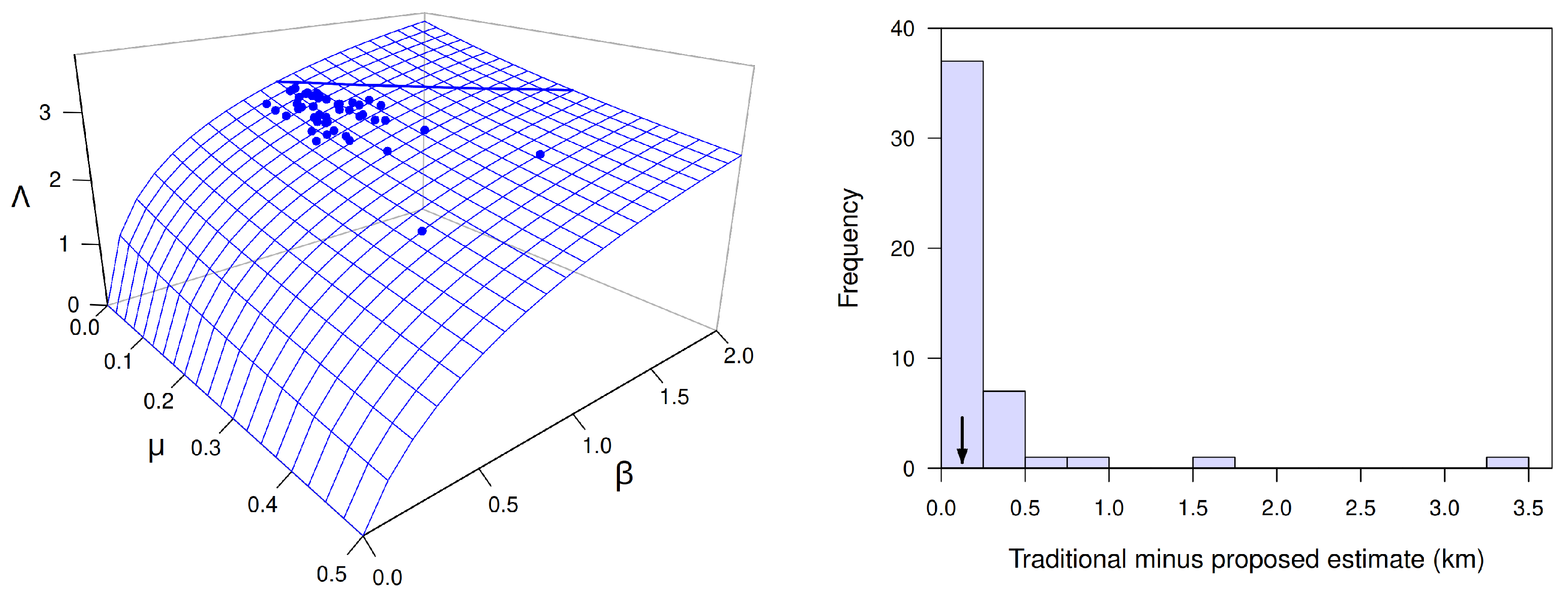
Figure 10 displays the key results. The left panel shows the values of $\Lambda$, calculated from estimates of $\beta$ and $\mu$, plotted on the portion of the $\Lambda$ surface shown in Figure 6 for values of $\beta$ between 0 and 2 and values of $\mu$ between 0 and $0.5$. Note that all values of $\Lambda$ are less than the traditional value of 3, implying that ${\mathcal{L}}_{95}$ is shorter than $L_{95}$. The right panel in Figure 10 shows a histogram of the difference $L_{95}-{\mathcal{L}}_{95}$ between the traditional and newly proposed estimates of the transition-zone length, all of which are positive. Nearly all of the 48 differences are less than $0.5$ km, and the median difference is $0.125$ km. One of the 48 estimates, however, is greater than $1.5$ km and another is greater than 3 km. These results suggest that the traditional estimate $L_{95}$ often will exceed the proposed estimate ${\mathcal{L}}_{95}$ by less than 200 m but occasionally will exceed it by more than a kilometer.

10. Characterizing the Transition Zone Based on DO Residence Time

An alternative approach to characterizing the length of the transition zone is to determine the residence-time distribution of dissolved oxygen in a slice of water as it moves downstream. As noted in Section 6, the residence time of a DO molecule is the time since the molecule entered the stream via photosynthesis or uptake from the atmosphere. For a slice of water that crossed upstream boundary $x=0$ of the focal reach at time $t_0$, the new DO at any time $t>t_0$ is simply the DO whose residence time is less than $t-t_0$.

10.1. The DO Residence-Time Distribution

The continuity equation governing the residence-time distribution of a slice of water has the same basic form as the continuity equation for the age distribution of a population, with the residence time of a DO molecule being analogous to its age, photosynthetic oxygen production and uptake from the atmosphere being analgous to immigration of age-0 neonates, and respiratory DO consumption and evasion of oxygen to the atmosphere being analogous to emigration. With the age analogy in mind, we will denote the residence time of a DO molecule by a. Let $c_{\mathrm{A}}(t,a;t_0)$ [Mass Length⁻³ Time⁻¹] for $a⩾0$ denote the DO residence-time distribution at time $t\ge t_0$ in a slice of water that entered the focal reach at time $t_0$. Assuming that DO with residence time a is respired in proportion to its relative concentration $c_{\mathrm{A}}(t,a;t_0)/C(t;t_0)$ in the slice, the DO residence-time distribution is governed by continuity equation

$${\displaystyle \frac{\partial c_{\mathrm{A}}}{\partial t}}+{\displaystyle \frac{\partial c_{\mathrm{A}}}{\partial a}}=-R(t;t_0)c_{\mathrm{A}}(t,a;t_0)/C(t;t_0)-K(t;t_0)c_{\mathrm{A}}(t,a;t_0)$$

(27)

for $t>t_0$ and $a>0$, subject to initial and boundary conditions

$$\begin{array}{ccc}\hfill c_{\mathrm{A}}(0,a;t_0)& =& I_{\mathrm{A}}(a;t_0),a⩾0\hfill \end{array}$$

(28)

$$\begin{array}{ccc}\hfill c_{\mathrm{A}}(t,0;t_0)& =& B_{\mathrm{A}}(t;t_0)=P(t;t_0)+K(t;t_0)C_{\mathrm{e}}(t;t_0),t>t_0\hfill \end{array}$$

(29)

where $C(t;t_0)$ is the solution of Equation (3) and is related to $c_{\mathrm{A}}(t,a;t_0)$ by

$$C(t;t_0)={\int }_0^{\infty }{c}_{\mathrm{A}}(t,a;t_0)da.$$

$C(t;t_0)$ represents the DO concentration at time t and location $\overline{u}(t-t_0)$ in a slice of water that entered the focal reach at time $t_0$, of which a portion $c_{\mathrm{A}}(t,a;t_0)da$ has residence-times between a and $a+da$. The right side of Equation (27) represents the sum of the intantaneous residence-time-specific “mortality” rate of DO via respiration (the first term) and “emigration” rate via evasion to the atmosphere (the second term). The boundary condition at residence time 0 in Equation (29) represents the instantaneous “immigration” rate of new DO via photosynthesis and invasion from the atmosphere (first and second terms on the right, respectively). (There is no term analogous to reproduction, because none of the new DO entering the stream is produced by DO that was already present.) The residence-time distribution and the processes that shape it are illustrated schematically in Figure 11.

10.2. Estimating the Transition Zone Length

In order to arrive at a simple analytical formula for the length of the transition zone, it is necessary to impose the same simplifying assumptions as in Section 6. Thus, we assume P, R, K, and $C_{\mathrm{e}}$ are all positive constants, which we interpret as averages over some suitable period of time such as a diel cycle. The characteristic base curves for Equation (27) are the lines given in parametric form by $t=t^{\prime }+\tau$ and $a=a^{\prime }+\tau$ for $t^{\prime }⩾t_0$, $a^{\prime }⩾0$, and $\tau ⩾0$. The solution of Equation (27) is

$$c_{\mathrm{A}}(t,a;t_0)=\left\{\begin{array}{cc}{c}_{\mathrm{A}}(0,a-(t-t_0);t_0)e^{-K(t-t_0)}{\left[1+{\beta }^{-1}\left(e^{K(t-t_0)}-1\right)\right]}^{-\mu },\hfill & t-t_0⩽a\hfill \\ (P+K{C}_{\mathrm{e}})C{(t;t_0)}^{-\mu }{e}^{-Ka}{\left[C^{*}{e}^{-Ka}+(C(t_0;t_0)-C^{*})e^{-K(t-t_0)}\right]}^{\mu },\hfill & t-t_0>a,\hfill \end{array}\right.$$

(30)

where $C^{*}=C_{\mathrm{e}}+(P-R)/K>0$, $\beta =C(t_0;t_0)/C^{*}$, and $\mu =R/K{C}^{*}$, as in Section 6. The part of the solution for which $t-t_0⩽a$ (i.e., residence times greater than or equal to the travel time from the upstream boundary) governs the fate of old DO that was present in the slice at time $t_0$ when it entered to focal stream reach at upstream boundary $x=0$. The other part of the solution (for residence times less than the travel time) governs the fate of new DO that entered the slice between times $t_0$ and t, within the focal reach.

The proportion of new DO in the slice at time t is given by

$${\displaystyle \frac{{\int }_0^{t-t_0}{c}_{\mathrm{A}}(t,a;t_0)da}{C(t;t_0)}}=1-{\left[{\displaystyle \frac{C(t_0;t_0)e^{-K(t-t_0)}}{C(t;t_0)}}\right]}^{1+\mu }.$$

Setting this proportion equal to p and solving for the implied travel time ${\mathcal{T}}_p=t-t_0$, we find that

$${\mathcal{T}}_p=\Lambda (p,\beta ,\mu )/K,$$

where $\Lambda (p,\beta ,\mu )$ is given by Equation (15). The corresponding travel distance ${\mathcal{L}}_p$, which is the length of the transition zone, is given by ${\mathcal{L}}_p={\mathcal{T}}_p\overline{u}$. That is,

$${\mathcal{L}}_p=\Lambda (p,\beta ,\mu )\overline{u}/K.$$

These formulas for ${\mathcal{T}}_p$ and ${\mathcal{L}}_p$ are identical to Equations (14) and (16), and we therefore use the same notation.

10.3. Stationary Distributions of DO Residence Time and Upstream Entry Distance

Equation (30) gives the residence time distribution of DO in a slice of water at time t that passed upstream reach boundary $x=0$ at time $t_0$. As t increases and the slice moves downstream, the implied residence-time distribution approaches a stationary distribution $c_{\mathrm{A}}^{*}\left(a\right)$. In reality, such a time-invariant distribution will not exist, because levels of solar irradiance, water temperature, stream flow, and so on will continually change, and also because stream habitat and community characteristics are longitudinally heterogeneous. However, it is still useful to examine the notional stationary distribution, because its simple form makes the main features of the actual residence-time distribution of DO obvious.

Letting $t\to \infty$ in the second part of the solution in Equation (30), or setting $\partial c_{\mathrm{A}}/\partial t=0$ in Equation (27) and solving, we find that the notional stationary DO residence-time distribution $c_{\mathrm{A}}^{*}\left(a\right)$ is given by

$$c_{\mathrm{A}}^{*}\left(a\right)=C^{*}(K+R/C^{*})e^{-(K+R/C^{*})a},a⩾0.$$

Expressed as a density function that integrates to unity, the normalized residence-time distribution $f_{\mathrm{A}}\left(a\right)=c_{\mathrm{A}}^{*}\left(a\right)/C^{*}$ is

$$f_{\mathrm{A}}\left(a\right)=(K+R/C^{*})e^{-(K+R/C^{*})a},a⩾0.$$

(31)

The function $f_{\mathrm{A}}\left(a\right)$ [Time⁻¹] is the probability density function for the residence time of a randomly chosen DO molecule in the moving slice of water. The corresponding survivor function (or complementary probability distribution function) ${\mathcal{F}}_{\mathrm{A}}\left(a\right)$ [dimensionless] is

$${\mathcal{F}}_{\mathrm{A}}\left(a\right)=e^{-(K+R/C^{*})a},a⩾0,$$

(32)

which represents the probability that the residence time of a randomly chosen DO molecule is greater than a.

The probability density and survivor functions in Equations (31) and (32) are related by $f_A\left(a\right)=-d{\mathcal{F}}_A\left(a\right)/da$. They are alternative, mathematically equivalent characterizations of an exponential distribution with mean DO residence time $\overline{a}$ given by

$$\overline{a}={\displaystyle \frac{1}{K+R/C^{*}}}<{\displaystyle \frac{1}{K}}.$$

(33)

Since $1/K$ is the notional mean DO residence time with no respiration (as assumed in the traditional estimate of the transition-zone length), Equation (33) states that respiration reduces the mean DO residence time, as it should. The DO residence-time distribution will be most strongly concentrated near zero when mean residence time $\overline{a}$ is small, which in turn will occur when the atmospheric exchange coefficient is high (e.g., shallow turbulent water) and the community respiration rate is high relative to the rates of photosynthesis and oxygen invasion from the atmosphere.

Under the plug-flow assumption, DO molecules of residence time a at the sonde entered the stream at distance $\overline{u}a$ upstream. Therefore, the residence time of a randomly chosen DO molecule at the sonde will be greater than a if and only if the upstream distance y at which the molecule entered the stream is greater than $\overline{u}a$. Equivalently, the upstream entry distance will be greater than y if and only if the residence time a is greater than $y/\overline{u}$. It follows at once from Equation (32) that the survivor function ${\mathcal{F}}_{\mathrm{Y}}$ for the upstream entry distance of a randomly chosen DO molecule at the sonde is

$${\mathcal{F}}_{\mathrm{Y}}\left(y\right)=e^{-{\displaystyle \frac{1}{\overline{u}}}(K+R/C^{*})y},y⩾0,$$

and the corresponding probability density function $f_{\mathrm{Y}}\left(y\right)$ [Length⁻¹] is

$$f_{\mathrm{Y}}\left(y\right)={\displaystyle \frac{1}{\overline{u}}}(K+R/C^{*})e^{-{\displaystyle \frac{1}{\overline{u}}}(K+R/C^{*})y},y⩾0.$$

Thus, the upstream entry distance has an exponential distribution with mean $\overline{y}$ given by

$$\overline{y}=\overline{u}\overline{a}={\displaystyle \frac{\overline{u}}{K+R/C^{*}}}<\overline{u}/K,$$

where $\overline{u}/K$ is the mean upstream entry distance for the notional case with no respiration. Recall, however, that these distributions for residence time and upstream entry distance are only approximate, since obtaining their simple forms required several rather strong simplifying assumptions, as in the case of the traditional estimate of transition-zone length.

Examples of the distributions of DO residence time and upstream entry distance are shown in Figure 12. The key property to note is that the density functions are maximal at DO residence time 0 and upstream entry distance 0 and decrease exponentially with increasing residence time and upstream entry distance. Within the transition zone, then, the greatest contribution to DO concentrations measured by a sonde is made by the stream habitat and community immediately upstream of the sonde, and the contribution declines exponentially (or roughly exponentially, in practice) with increasing distance upstream. A practical implication is that in choosing a location for a sonde, it is particularly important to ensure that the portion of the focal reach immediately upstream is representative of the entire reach.

11. Discussion

As noted in the Introduction, streams often consist of a longitudinal sequence of more-or-less distinct reaches dominated by different habitat and community types, each with its own characteristic community metabolism. As the flowing water exits one reach and enters the next, there is a transition zone in which physical and chemical properties of the water, such as temperature and DO concentration, change from being representative of the upstream reach to being representative of the downstream reach. The theoretical approaches we have developed provide practical ways to estimate the length of this transition zone for DO. Rutherford et al. [42,43] address the corresponding problem for water temperature.

The extent of the DO transition zone between one stream reach and the next is important in metabolism studies employing the FWDO method with 1-station monitoring, since this method derives its metabolism estimates from time series acquired at a single location per reach. If a sonde is placed so close to the upstream boundary of the focal reach that it lies well within the transition zone, the DO time series it acquires may largely reflect DO that entered the stream upstream of the focal reach rather than within it. Another way to say this is that the reach actually being monitored may extend well upstream of the focal reach. Viewed either way, it clearly is unlikely in this case that metabolism estimates based on time series acquired by the sonde will mainly reflect the habitat and community type in the focal reach.

Obtaining metabolism estimates that are representative of specific types of stream habitat is important in characterizing and comparing streams. The well-known longitudinal patterns of change in stream and river habitat over long distances are a central part of the river continuum concept of Vannote et al. [62]. These patterns require that useful comparisons between streams be stratified in order to control for position within the river continuum as indicated by stream order or magnitude. Otherwise, effects of the large-scale trend of changing habitat conditions along lengthy streams and rivers (e.g., water depth, light attenuation, current velocity, suspended particulate matter, shading by riparian vegetation) are confounded with effects of other properties (e.g., local climate, anthropogenic stressors) that can affect stream ecosystem function. It is also important to be aware that marked changes in stream habitat can occur even over short distances (e.g., shifts between shaded and unshaded reaches, or between riffles and pools), and these can have pronounced effects on local stream metabolism at a given position within the river continuum (e.g., [2]).

In addition to its importance for studies of stream metabolism, the length of the transition zone is also important in studies concerned specifically with predicting stream DO concentrations and how they will respond to potential management options. This, of course, is the problem addressed by the original Streeter-Phelps model for cases where metabolism is dominated by catabolism of allochthonous organic matter discharged to a river by upstream point sources. Another example is the design of stream restoration projects to improve fish habitat, where both DO concentration and water temperature may be important. The key point is that the temperature and DO concentration at a given stream location are strongly influenced by habitat upstream of the location. This dependence must be accounted for in estimating and interpreting components of stream metabolism via the FWDO method, or in designing stream restoration projects to improve DO or temperature conditions in a particular reach.

In studies of stream metabolism, the length of the transition zone is an important constraint on where the sonde should be placed within a focal reach when 1-station monitoring is used. Another important consideration is whether the length of a focal reach and the longitudinal pattern of change in DO concentration within it is suitable for estimating components of metabolism. This problem is discussed by Grace and Imberger [26] and Reichert et al. [21], among others. For example, 2-station monitoring often fails to produce plausible estimates of metabolism if the distance between the two sondes is so short, relative to the current velocity and the rates of metabolism and atmospheric exchange, that little change in DO concentration occurs between them [26]. In the case of 1-station monitoring, it is commonly noted that obtaining reliable estimates of metabolism components requires the longitudinal profile of DO concentration to be approximately uniform (flat) in the vicinity of the sonde (e.g., [26]). More precisely, this form of the FWDO method assumes that $\partial c/\partial x=0$ in the fundamental continuity equation stated in Equation (2), and that the gas-exchange equilibrium and the photosynthesis, respiration, and atmospheric exchange rates all depend on time t but not on location x within the reach. The DO continuity equation then reduces to the simpler ordinary differential equation,

$${\displaystyle \frac{dc}{dt}}=\phi \left(t\right)-\rho \left(t\right)+\kappa \left(t\right)\left(c_{\mathrm{e}}\left(t\right)-c\left(t\right)\right),$$

which is the basis for estimating parameter values from DO and temperature time series when 1-station monitoring is used.

The requirement that $\partial c/\partial x=0$ (approximately) in the vicinity of each sonde in metabolism studies employing 1-station monitoring imposes a second constraint on admissible sonde locations, in addition to that imposed by the length of the transition zone. To illustrate the relationship between these two constraints, we briefly consider the conditions under which the longitudinal profile of DO concentration will be approximately uniform in the vicinity of a sonde. We have already mentioned this problem in discussing the basis of the traditional estimate $L_{95}$ of the transition-zone length in Section 8, since this is actually the problem that Chapra and Di Toro [60] claim their commonly-cited estimate addresses. We now consider it more carefully to clarify the meaning of Chapra and Di Toro’s result, which turns out to be somewhat different than these authors suggest.

Given the usual model of stream DO transport and dynamics outlined in Section 5, and replacing the various process rates with averages over a suitable time period (e.g., a diel cycle), the longitudinal profile of DO concentration $c(t,x)$ will converge to a stationary pattern $c^{*}\left(x\right)$ as t becomes large. In reality, such a stationary pattern will never be attained, mainly because of the pronounced diel cycle in solar irradiance which, directly and indirectly, forces diel changes in rates of the various processes that tend to increase and decrease stream DO concentrations. Nevertheless, the constant-rate approximation to the model of DO transport and dynamics provides useful approximations to results of the variable-rate model, as we saw in Section 7 for estimates of the transition-zone length.

One way to find the stationary longitudinal DO profile $c^{*}\left(x\right)$ is by setting $\partial c/\partial t=0$ in Equation (2). To prevent dependence of the results on physical dimensions, we introduce dimensionless variables $\widehat{x}=\kappa x/\overline{u}$ and $\widehat{c}\left(\widehat{x}\right)=c^{*}(\overline{u}\widehat{x}/\kappa )/c^{*}(\infty )$ in the resulting differential equation. Solving this equation (see Appendix B), we find that the absolute value of the slope of the dimensionless longitudinal DO profile $\widehat{c}\left(\widehat{x}\right)$ is given by

$$|d\widehat{c}/d\widehat{x}|=|\beta -1|e^{-\widehat{x}},$$

(34)

where dimensionless parameter $\beta =c^{*}\left(0\right)/c^{*}(\infty )$ (which is consistent with the definition of $\beta$ in Equation (11)). The absolute value of the slope is therefore greatest at the upstream boundary of the focal reach and decreases exponentially with increasing dimensionless distance $\widehat{x}$ downstream.

Let ${\widehat{x}}_{\epsilon }$ denote the minimum value of $\widehat{x}$ such that $|d\widehat{c}/d\widehat{x}|⩽\epsilon$, where $\epsilon$ is a positive dimensionless number much smaller than unity. Clearly ${\widehat{x}}_{\epsilon }=0$ if $|\beta -1|⩽\epsilon$. Otherwise, ${\widehat{x}}_{\epsilon }={log}_e\left({\epsilon }^{-1}|\beta -1|\right)$. The corresponding dimensional distance $x_{\epsilon }={\widehat{x}}_{\epsilon }\overline{u}/\kappa$ is therefore given by

$$\begin{array}{c}\hfill x_{\epsilon }=\left\{\begin{array}{cc}0,\hfill & \mathrm{if}|\beta -1|⩽\epsilon \hfill \\ {log}_e\left({\epsilon }^{-1}|\beta -1|\right)\overline{u}/\kappa >0,\hfill & \mathrm{if}|\beta -1|>\epsilon .\hfill \end{array}\right.\end{array}$$

Thus, if the DO concentration $c^{*}\left(0\right)$ of water entering the focal reach is already close enough to $c^{*}(\infty )$ so that $|\beta -1|⩽\epsilon$, then the slope of the DO profile will be sufficiently close to zero for all $x⩾0$ and there is no constraint on the location of the sonde. But if the initial DO concentration is substantially different from $c^{*}(\infty )$, then $x_{\epsilon }>0$ and its value will be greater, the greater the initial discrepancy measure $|\beta -1|$ is.

As an example, if we choose $\epsilon =0.05$, and if $|\beta -1|>\epsilon$, then

$$x_{0.05}\approx 3\overline{u}/\kappa +{log}_e\left(\right|\beta -1\left|\right)\overline{u}/\kappa .$$

This estimate may be compared with that of Chapra and Di Toro [60], which is the same as the traditional estimate of the transition-zone length in Equation (1). Their estimate does not depend on the magnitude of the initial discrepancy between $c^{*}\left(0\right)$ and $c^{*}(\infty )$, which is physically incorrect (unless one argues that $\beta =2$, which is physically unjustified). The estimate of Chapra and Di Toro actually tells us the distance at which the discrepancy $c^{*}\left(x\right)-c^{*}(\infty )$ at downstream distance x first becomes sufficiently small relative to initial discrepancy $c^{*}\left(0\right)-c^{*}(\infty )$. This is an appropriate distance-based measure of the relative responsiveness of the stream ecosystem to displacements from steady state but is not appropriate as a measure of the absolute distance at which $c^{*}\left(x\right)$ becomes approximately constant, which clearly depends on the magnitude of the initial discrepancy.

When employing the FWDO method with 1-station monitoring to estimate components of stream metabolism in a particular reach, length estimates $x_{\epsilon }$ and ${\mathcal{L}}_p$ impose two constraints that jointly determine the allowable locations for the sonde. One of these constraints—the main focus of the present paper—assures that the time series of DO concentrations acquired by the sonde mainly reflects the stream community in the focal reach. The other assures that the longitudinal profile of DO concentration is approximately flat in the vicinity of the sonde, which is a condition for obtaining valid metabolism estimates with 1-station monitoring. Both constraints must be satisfied if metabolism estimates based on the acquired time series are to be valid and attributable to the focal reach. To satisfy both constraints, the distance $x_{\mathrm{S}}$ between the upstream boundary of the focal reach and the sonde must be at least as large as both ${\mathcal{L}}_p$ and $x_{\epsilon }$ for suitable choices of p and $\epsilon$. That is,

$$x_{\mathrm{S}}⩾max({\mathcal{L}}_p,x_{\epsilon }).$$

(35)

If the sonde is placed closer than $max({\mathcal{L}}_p,x_{\epsilon })$ to the upstream boundary of the focal reach, then the FWDO method with 1-station monitoring will yield unreliable estimates of the components of community metabolism in the focal reach. A corollary is that it will not be possible to obtain reliable estimates if the total length of the focal reach is less than $max({\mathcal{L}}_p,x_{\epsilon })$.

Two extreme cases are instructive. First, note that $\beta$ approaches zero as $c^{*}\left(0\right)$ does (with $c^{*}(\infty )$ fixed). It follows from Equation (15) that ${lim}_{c^{*}\left(0\right)\to 0}\Lambda =0$, and therefore ${lim}_{c^{*}\left(0\right)\to 0}{\mathcal{L}}_{95}=0$. This case addresses the artificial but conceptually important case where the DO concentration of water entering the focal reach is approximately zero, and all DO at every location within the reach is therefore new. It follows that the first constraint will be satisfied regardless of where the sonde is placed within the focal reach, so only the second constraint restricts placement of the sonde. The other extreme case is where $c^{*}\left(0\right)=c^{*}(\infty )$. Here, $\beta =1$ and $|d\widehat{c}/d\widehat{x}|=0$ for all $\widehat{x}$ in Equation (34), so $x_{\epsilon }=0$. In this case, then, the slope of the longitudinal DO profile is zero at all locations within the focal reach, so only the first constraint restricts placement of the sonde. Aside from these extreme cases, both constraints impose significant restrictions on sonde placement, and the condition in Equation (35) becomes nontrivial.

But how should the values of thresholds p and $\epsilon$ in ${\mathcal{L}}_p$ and $x_{\epsilon }$ be chosen? As we have indicated in previous sections of this paper, the traditional choice of p is $0.95$. Our own subjective view is that this value is probably higher than necessary and should be regarded as conservative. On subjective grounds, we also suggest that $0.05$ is a reasonable choice for $\epsilon$, but we have no evidence that this value is small enough to be conservative. Objective evidence for appropriate values of p and $\epsilon$ must come from numerical studies in which a specific statistical method is employed for estimating components of metabolism from artificial time series generated by models like the one presented in Section 7, with random noise added. In this way, the true values of photosynthesis, respiration, and atmospheric exchange parameters will be known and the error resulting from estimating these parameters from time series acquired at different distances from the upstream boundary of the focal reach can therefore be rigorously quantified. Numerical values of thresholds p and $\epsilon$ that are protective but not overly so can then be determined. This task, however, is beyond the scope of the present paper.

12. Conclusions

We now briefly summarize the main takeaways from our study.

• The traditional estimate $L_{95}$ of the transition-zone length accounts for loss of old DO via evasion to the atmosphere across the air-water interface but does not account for loss of old DO via aerobic respiration or gain of new DO via oxygenic photosynthesis and invasion from the atmosphere.
• The proposed alternative estimate ${\mathcal{L}}_{95}$ in Equation (16) accounts for all three of the main processes by which old DO is lost from a stream and new DO is gained: photosynthesis, respiration, and atmospheric exchange.
• Though it is theoretically possible for the proposed estimate of transition-zone length to exceed the traditional estimate, application to FWDO data for 10 streams in eastern New York state showed that ${\mathcal{L}}_{95}<L_{95}$ in all cases (Figure 10).
• DO concentrations measured by a sonde are most heavily influenced by the portion of the focal reach immediately upstream of the sonde (Figure 12, right panel). Therefore, in order for estimates of metabolic rates obtained with 1-station monitoring to be representative of the focal reach, it is particularly important to avoid placing the sonde in an area where the habitat and benthic community are clearly not representative of the reach.