
Multi-Output Machine-Learning Prediction of Volatile Organic Compounds (VOCs): Learning from Co-Emitted VOCs

 ,
,  ,
,  ,
,
Abstract
1. Introduction
2. Literature Review
3. Materials and Methods
3.1. Dataset
3.2. Target VOCs
3.3. Predictors
3.4. ML Models
3.4.1. Multi-Output Gaussian Process Regression (MOGP)
3.4.2. Neural Network Multi-Output Regression
3.4.3. CatBoost Multi-Output Regression
3.5. Assessment of Predictive Performance
3.5.1. Coefficient of Determination (R2)
3.5.2. Root Mean Square Error (RMSE)
3.5.3. Mean Absolute Error (MAE)
3.6. Feature Importance
4. Results
4.1. Evaluation of the Ability of Machine-Learning Models to Predict Multiple VOCs Simultaneously
Overfitting Evaluation
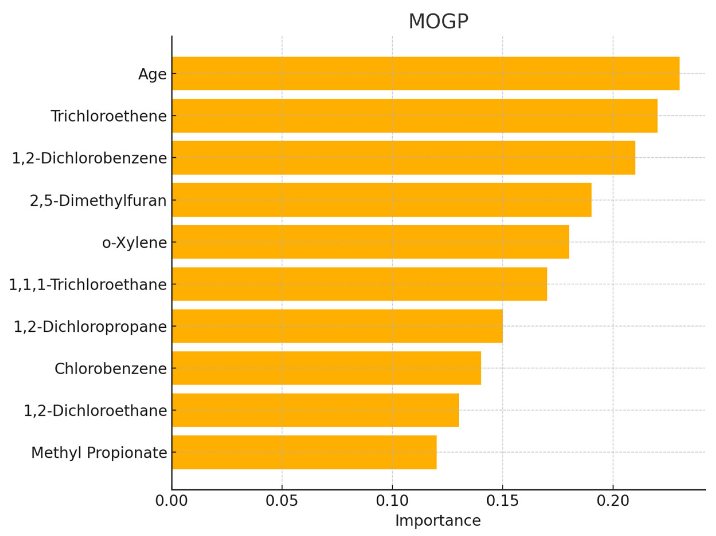
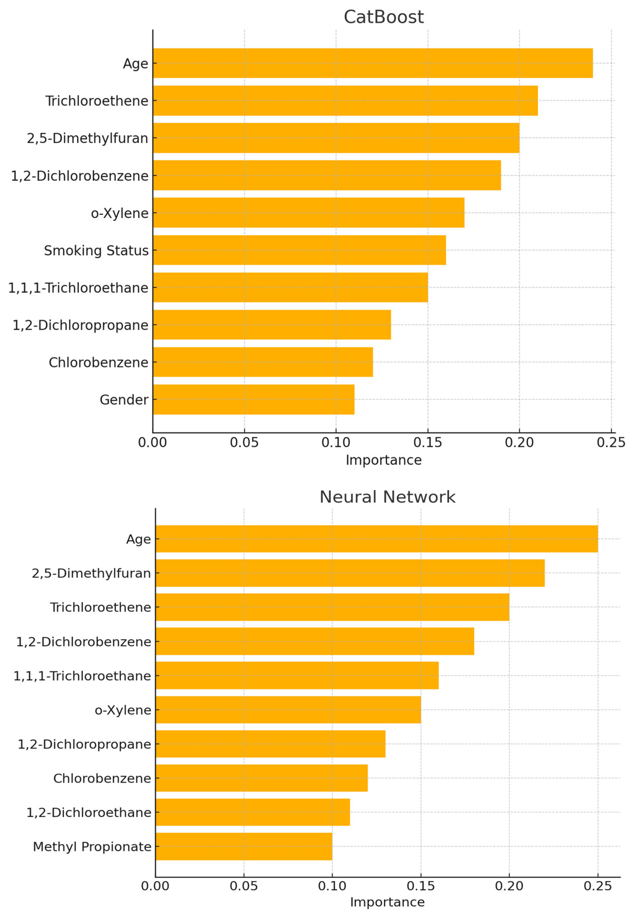
4.2. Results of Feature Importance Analysis
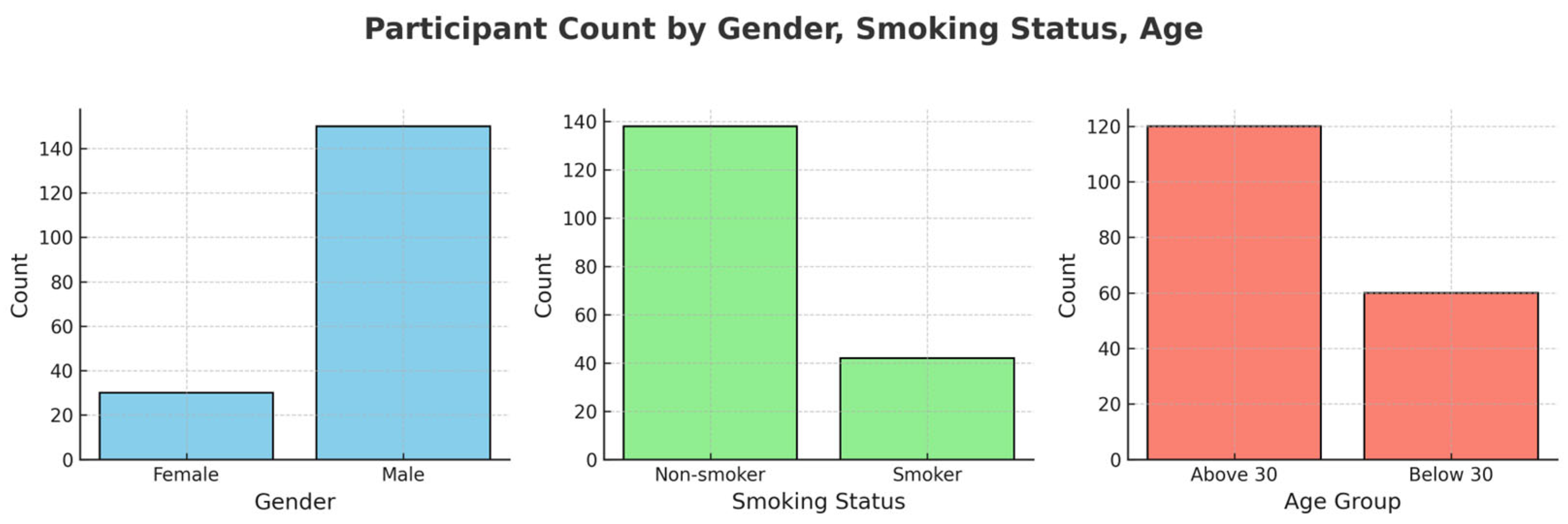
4.3. Identification of High-Risk Groups
4.4. Study Limitations
5. Conclusions
Author Contributions
Funding
Institutional Review Board Statement
Informed Consent Statement
Data Availability Statement
Acknowledgments
Conflicts of Interest
Appendix A

| Analyte | Structure | CAS Number |
|---|---|---|
| acetonitrile |  | 75-05-8 |
| ethyl acetate |  | 141-78-6 |
| 1,1-Dichloroethene |  | 75-35-4 |
| 2-propenal |  | 107-02-8 |
| Methylene chloride |  | 75-09-2 |
| Transe-1,2-Di Dichloroethene |  | 156-60-5 |
| propanal |  | 123-38-6 |
| Methyl tert-butyl ether |  | 1634-04-4 |
| Methyl acetate |  | 79-20-9 |
| cis-1,2-Dichloroethene |  | 156-59-2 |
| chloroform |  | 67-66-3 |
| 1,2-Dichloroethane |  | 107-06-2 |
| 1,1,1-Trichloroethane |  | 71-55-6 |
| Carbon tetrachloride |  | 56-23-5 |
| Benzene |  | 71-43-2 |
| Dibromomethane |  | 74-95-3 |
| 1,2-Dichloropropane |  | 78-87-5 |
| Trichloroethene |  | 79-01-6 |
| Bromodichloromethane | 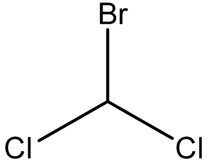 | 75-27-4 |
| Methyl proprionate |  | 554-12-1 |
| 2,5-Dimethylfuran | 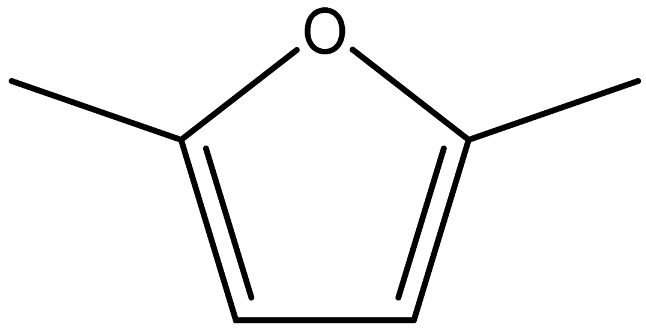 | 625-86-5 |
| 1,1,2-Trichloroethane | 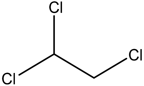 | 79-00-5 |
| n-butyl acetate | 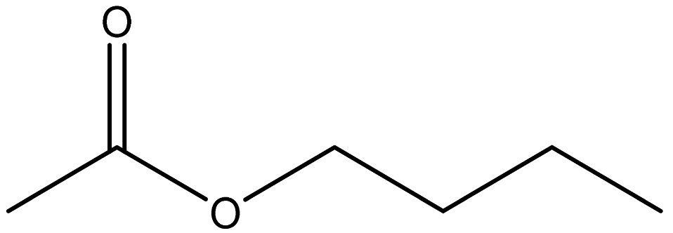 | 123-86-4 |
| Toluene |  | 108-88-3 |
| Dibromochloromethane |  | 124-48-1 |
| Tetrachloroethene |  | 127-18-4 |
| Chlorobenzene |  | 108-90-7 |
| Ethylbenzene |  | 100-41-4 |
| p-Xylene |  | 179601-23-1 |
| Bromoform |  | 75-25-2 |
| Styrene |  | 100-42-5 |
| 1,1,2,2-Tetrachlroethane |  | 79-34-5 |
| o- Xylene |  | 95-47-6 |
| 1,3-Dichlorobenzene |  | 541-73-1 |
| 1,2-Dichlorobenzene |  | 95-50-1 |
| 1,4-Dichlorobenzene |  | 106-46-7 |
| toluene 2,4- diisocyanate |  | 584-84-9 |
| Hexachloroethane |  | 67-72-1 |
| Age | Gender | Smoking Status | ||||||||||
|---|---|---|---|---|---|---|---|---|---|---|---|---|
| ≤15 | >15 | Male | Female | Non-Smoker | Smoker | |||||||
| VOC | Mean | Std | Mean | Std | Mean | Std | Mean | Std | Mean | Std | Mean | Std |
| acetonitrile | 48.64 | 1.76 | 61.09 | 3.78 | 56.61 | 7.25 | 58.56 | 2.24 | 55.06 | 6.30 | 63.10 | 3.46 |
| n-butyl acetate | 32.50 | 1.00 | 40.44 | 2.64 | 37.69 | 4.75 | 38.31 | 1.06 | 36.45 | 4.03 | 42.23 | 1.67 |
| Toluene | 76.34 | 1.02 | 84.87 | 5.44 | 82.57 | 6.44 | 79.30 | 1.31 | 79.71 | 4.25 | 89.63 | 4.55 |
| p-Xylene | 62.44 | 2.42 | 68.81 | 2.93 | 66.73 | 4.33 | 66.46 | 2.57 | 65.42 | 3.65 | 70.84 | 2.27 |
| Toluene 2 4-diisocyanate | 123.93 | 11.39 | 275.35 | 35.93 | 222.02 | 84.46 | 239.15 | 16.63 | 199.36 | 70.29 | 308.73 | 19.89 |
| Age | Gender | Smoking Status | ||||||||||
|---|---|---|---|---|---|---|---|---|---|---|---|---|
| ≤15 | >15 | Male | Female | Non-Smoker | Smoker | |||||||
| VOC | Mean | Std | Mean | Std | Mean | Std | Mean | Std | Mean | Std | Mean | Std |
| acetonitrile | 49.46 | 1.30 | 60.71 | 3.13 | 56.67 | 6.434 | 58.42 | 1.760 | 55.28 | 5.65 | 62.50 | 2.55 |
| n-butyl acetate | 33.08 | 0.84 | 40.27 | 2.304 | 37.74 | 4.26 | 38.51 | 0.820 | 36.61 | 3.52 | 42.01 | 1.52 |
| Toluene | 77.10 | 0.783 | 84.66 | 4.79 | 82.58 | 5.70 | 79.95 | 1.166 | 80.08 | 3.68 | 88.92 | 4.07 |
| p-Xylene | 63.11 | 1.54 | 68.88 | 2.44 | 66.97 | 3.74 | 66.91 | 1.75 | 65.78 | 2.97 | 70.83 | 1.93 |
| Toluene 2 4-diisocyanate | 135.69 | 9.93 | 270.21 | 33.36 | 222.88 | 75.58 | 237.83 | 13.48 | 202.13 | 62.08 | 301.73 | 18.86 |
References
- Nawaz, F.; Ali, M.; Ahmad, S.; Yong, Y.; Rahman, S.; Naseem, M.; Hussain, S.; Razzaq, A.; Khan, A.; Ali, F.; et al. Carbon based nanocomposites, surface functionalization as a promising material for VOCs (volatile organic compounds) treatment. Chemosphere 2024, 364, 143014. [Google Scholar] [CrossRef] [PubMed]
- Gao, M.; Liu, W.; Wang, H.; Shao, X.; Shi, A.; An, X.; Li, G.; Nie, L. Emission factors and characteristics of volatile organic compounds (VOCs) from adhesive application in indoor decoration in China. Sci. Total Environ. 2021, 779, 145169. [Google Scholar] [CrossRef] [PubMed]
- Halios, C.H.; Landeg-Cox, C.; Lowther, S.D.; Middleton, A.; Marczylo, T.; Dimitroulopoulou, S. Chemicals in European residences–Part I: A review of emissions, concentrations and health effects of volatile organic compounds (VOCs). Sci. Total Environ. 2022, 839, 156201. [Google Scholar] [CrossRef] [PubMed]
- Khan, A.; Kanwal, H.; Bibi, S.; Mushtaq, S.; Khan, A.; Khan, Y.H.; Mallhi, T.H. Volatile organic compounds and neurological disorders: From exposure to preventive interventions. In Environmental Contaminants and Neurological Disorders; Springer: Cham, Switzerland, 2021; pp. 201–230. [Google Scholar]
- Tsai, W.-T. An overview of health hazards of volatile organic compounds regulated as indoor air pollutants. Rev. Environ. Health 2019, 34, 81–89. [Google Scholar] [CrossRef]
- Kanwal, S.; Abas, N. VOC exposure in Pakistani furniture-painting micro-workshops: Role of inadequate ventilation. Indoor Air 2024, 34, e13234. [Google Scholar] [CrossRef]
- Kim, Y.; Park, J. Measurements of solvent-based coating VOCs in small wood-craft shops. J. Occup. Health 2023, 65, e12301. [Google Scholar] [CrossRef]
- Ranjan, S.; Chaitali, R.; Sinha, S.K. Gas chromatography-mass–mass spectrometry (GC-MS): A comprehensive review of synergistic combinations and their applications in the past two decades. J. Anal. Sci. Appl. Biotechnol. 2023, 5, 72–85. [Google Scholar]
- Zhang, J.D.; Le, M.N.; Hill, K.J.; Cooper, A.A.; Stuetz, R.M.; Donald, W.A. Identifying robust and reliable volatile organic compounds in human sebum for biomarker discovery. Anal. Chim. Acta 2022, 1233, 340506. [Google Scholar] [CrossRef]
- Baum, J.L.R. Design of Non-Invasive Systems for Detection of Exogenous and Endogenous Volatile Compounds for Applications in Environmental Exposure and Health Diagnostics. Doctoral Dissertation, University of Miami, Coral Gables, FL, USA, 2020. [Google Scholar]
- Fanti, G.; Borghi, F.; Spinazzè, A.; Rovelli, S.; Campagnolo, D.; Keller, M.; Cattaneo, A.; Cauda, E.; Cavallo, D.M. Features and practicability of the next-generation sensors and monitors for exposure assessment to airborne pollutants: A systematic review. Sensors 2021, 21, 4513. [Google Scholar] [CrossRef]
- Alyami, A.R. Assessment of occupational exposure to gasoline vapour at petrol stations. Doctoral Dissertation, Cranfield University, Bedford, UK, 2016. [Google Scholar]
- Romieu, I.; Ramirez, M.; Meneses, F.; Ashley, D.; Lemire, S.; Colome, S.; Fung, K.; Hernandez-Avila, M. Environmental exposure to volatile organic compounds among workers in Mexico City as assessed by personal monitors and blood concentrations. Environ. Health Perspect. 1999, 107, 511–515. [Google Scholar] [CrossRef]
- Vardoulakis, S. Human exposure: Indoor and outdoor. Issues Environ. Sci. Technol. 2009, 28, 85. [Google Scholar]
- Kuykendall, J.R.; Shaw, S.L.; Paustenbach, D.; Fehling, K.; Kacew, S.; Kabay, V. Chemicals present in automobile traffic tunnels and the possible community health hazards: A review of the literature. Inhal. Toxicol. 2009, 21, 747–792. [Google Scholar] [CrossRef] [PubMed]
- Klepeis, N.E. Modeling human exposure to air pollution. Hum. Expo. Anal. 2006, 445–470. [Google Scholar]
- Salo, L. The Effects of Coatings on the Indoor air Emissions of Wood Board. Master’s Thesis, Insinööritieteiden korkeakoulu, Espoo, Finland, 2017. [Google Scholar]
- Christopher, A. Identification and Assessment of Indoor Air Quality Exposures at a Manufacturing Facility. Master’s Thesis, College of Charleston, Charleston, SC, USA, 2024. [Google Scholar]
- Woolley, T. Building Materials, Health and Indoor Air Quality; Routledge: Abingdon, UK, 2024; Volume 2. [Google Scholar]
- Kelleher, S.; Quinn, C.; Miller-Lionberg, D.; Volckens, J. A low-cost particulate matter (PM 2.5) monitor for wildland fire smoke. Atmos. Meas. Tech. 2018, 11, 1087–1097. [Google Scholar] [CrossRef]
- Epping, R.; Koch, M. On-site detection of volatile organic compounds (VOCs). Molecules 2023, 28, 1598. [Google Scholar] [CrossRef]
- Masmoudi, S.; Elghazel, H.; Taieb, D.; Yazar, O.; Kallel, A. A machine-learning framework for predicting multiple air pollutants’ concentrations via multi-target regression and feature selection. Sci. Total Environ. 2020, 715, 136991. [Google Scholar] [CrossRef]
- Liu, S.; Li, R.; Wild, R.J.; Warneke, C.; De Gouw, J.A.; Brown, S.S.; Miller, M.; Luongo, J.C.; Jimene, J.L.; Ziemann, P.J. Contribution of human-related sources to indoor volatile organic compounds in a university classroom. Indoor Air 2016, 26, 925–938. [Google Scholar] [CrossRef]
- Sheu, R.; Lin, M. Multi-surrogate regression to predict benzene toluene from co-emitted VOCs + meteorology. Atmosphere 2023, 14, 1145. [Google Scholar] [CrossRef]
- Manh, L.H. Machine Learning for Ultraviolet Spectral Prediction. Doctoral Dissertation, The University of Texas at Arlington, Arlington, TX, USA, 2023. [Google Scholar]
- Huynh, N.; Ludkovski, M. Multi-output Gaussian processes for multi-population longevity modelling. Ann. Actuar. Sci. 2021, 15, 318–345. [Google Scholar] [CrossRef]
- Eid, A.; Jodeh, S.; Chakir, A.; Hanbali, G.; Roth, E. Machine learning-based analysis of workers’ exposure and detection to volatile organic compounds (VOC). Int. J. Environ. Sci. Technol. 2025, 22, 1–17. [Google Scholar] [CrossRef]
- Liu, J.; Zhang, R.; Xiong, J. Machine learning approach for estimating the human-related VOC emissions in a university classroom. In Building Simulation; Tsinghua University Press: Beijing, China, 2023; Volume 16, pp. 915–925. [Google Scholar]
- Juarez, E.K.; Petersen, M.R. A comparison of machine learning methods to forecast tropospheric ozone levels in Delhi. Atmosphere 2021, 13, 46. [Google Scholar] [CrossRef]
- Bainomugisha, E.; Warigo, P.A.; Daka, F.B.; Nshimye, A.; Birungi, M.; Okure, D. AI-driven environmental sensor networks and digital platforms for urban air pollution monitoring and modelling. Soc. Impacts 2024, 3, 100044. [Google Scholar] [CrossRef]
- Sané, F.C.E.; Mbaye, M.; Gueye, B. Edge-AI for Monitoring Air Pollution from Urban Waste Incineration: A Survey. In IoT Edge Intelligence; Springer Nature Switzerland: Cham, Switzerland, 2024; pp. 335–363. [Google Scholar]
- Yang, J.; Hu, X.; Feng, L.; Liu, Z.; Murtazt, A.; Qin, W.; Zhou, M.; Liu, J.; Bi, Y.; Qian, J.; et al. AI-Enabled Portable E-Nose Regression Predicting Harmful Molecules in a Gas Mixture. ACS Sens. 2024, 9, 2925–2934. [Google Scholar] [CrossRef]
- Koçak, E. Comprehensive evaluation of machine learning models for real-world air quality prediction and health risk assessment by AirQ+. Earth Sci. Inform. 2025, 18, 1–17. [Google Scholar] [CrossRef]
- Shi, G.; Du, H.; Du, L.; Ni, X.; Hu, Y.; Pang, D.; Yao, L. Distribution characteristics of volatile organic compounds and its multidimensional impact on ozone formation in arid regions based on machine learning algorithms. Environ. Pollut. 2025, 373, 126159. [Google Scholar] [CrossRef]
- Popescu, S.M.; Mansoor, S.; Wani, O.A.; Kumar, S.S.; Sharma, V.; Sharma, A.; Arya, V.M.; Kirkham, M.B.; Hou, D.; Bolan, N.; et al. Artificial intelligence and IoT driven technologies for environmental pollution monitoring and management. Front. Environ. Sci. 2024, 12, 1336088. [Google Scholar] [CrossRef]
- Rane, N.; Choudhary, S.; Rane, J. Leading-Edge Artificial Intelligence (AI), Machine Learning (ML), Blockchain, and Internet of Things (IoT) Technologies for Enhanced Wastewater Treatment Systems. 2023. Available online: https://papers.ssrn.com/sol3/papers.cfm?abstract_id=4641557 (accessed on 25 May 2025).
- Akinosho, T.D.; Bilal, M.; Hayes, E.T.; Ajayi, A.; Ahmed, A.; Khan, Z. Deep learning-based multi-target regression for traffic-related air pollution forecasting. Mach. Learn. Appl. 2023, 12, 100474. [Google Scholar] [CrossRef]
- Ye, H.; Du, Z.; Lu, H.; Tian, J.; Chen, L.; Lin, W. Using machine learning methods to predict VOC emissions in chemical production with hourly process parameters. J. Clean. Prod. 2022, 369, 133406. [Google Scholar] [CrossRef]
- Hashemitaheri, M.; Ebrahimi, E.; de Silva, G.; Attariani, H. Optical sensor for BTEX detection: Integrating machine learning for enhanced sensing. Adv. Sens. Energy Mater. 2024, 3, 100114. [Google Scholar] [CrossRef]
- Kang, M.; Han, J.; Kim, Y.; Kim, S.; Kang, S. Data-driven autonomous operation of VOCs removal system. Sci. Rep. 2024, 14, 5953. [Google Scholar] [CrossRef]
- Zhang, R.; Wang, H.; Tan, Y.; Zhang, M.; Zhang, X.; Wang, K.; Ji, W.; Sun, L.; Yu, X.; Zhao, J.; et al. Using a machine learning approach to predict the emission characteristics of VOCs from furniture. Build. Environ. 2021, 196, 107786. [Google Scholar] [CrossRef]
- Rasmussen, C.E.; Williams, C. Gaussian Processes for Machine Learning; The Mit Press: Cambridge, MA, USA, 2006; Volume 32, p. 68. [Google Scholar]
- Lundberg, S.M.; Lee, S.-I. A unified approach to interpreting model predictions. Adv. Neural Inf. Process. Syst. 2017, 30, 4765–4774. [Google Scholar]
- Jodeh, S.; Chakir, A.; Hanbali, G.; Roth, E.; Eid, A. Method Development for Detecting Low Level Volatile Organic Compounds (VOCs) among Workers and Residents from a Carpentry Work Shop in a Palestinian Village. Int. J. Environ. Res. Public Health 2023, 20, 5613. [Google Scholar] [CrossRef] [PubMed]
- Win-Shwe, T.-T.; Fujimaki, H. Neurotoxicity of toluene. Toxicol. Lett. 2010, 198, 93–99. [Google Scholar] [CrossRef]
- Frick-Engfeldt, M.; Zimerson, E.; Karlsson, D.; Marand, A.; Skarping, G.; Isaksson, M.; Bruze, M. Chemical analysis of 2, 4-toluene diisocyanate, 1, 6-hexamethylene diisocyanate, and isophorone diisocyanate in petrolatum patch-test preparations. DERM 2005, 16, 130–135. [Google Scholar]
- Tomas, R.A.; Bordado, J.o.C.; Gomes, J.F. p-Xylene oxidation to terephthalic acid: A literature review oriented toward process optimization and development. Chem. Rev. 2013, 113, 7421–7469. [Google Scholar] [CrossRef]
- Wang, Y.; Chen, Z.; Haefner, M.; Guo, S.; DiReda, N.; Ma, Y.; Avedisian, C.T. Combustion of n-butyl acetate synthesized by a new and sustainable biological process and comparisons with an ultrapure commercial n-butyl acetate produced by conventional Fischer esterification. Fuel 2021, 304, 121324. [Google Scholar] [CrossRef]
- McConvey, I.F.; Woods, D.; Lewis, M.; Gan, Q.; Nancarrow, P. The importance of acetonitrile in the pharmaceutical industry and opportunities for its recovery from waste. Org. Process Res. Dev. 2012, 16, 612–624. [Google Scholar] [CrossRef]
- Liu, M.; Chowdhary, G.; Da Silva, B.C.; Liu, S.Y.; How, J.P. Gaussian processes for learning and control: A tutorial with examples. IEEE Control. Syst. Mag. 2018, 38, 53–86. [Google Scholar] [CrossRef]
- Álvarez, M.A.; Rosasco, L.; Lawrence, N.D. Kernels for vector-valued functions: A review. Found. Trends® Mach. Learn. 2012, 4, 195–266. [Google Scholar] [CrossRef]
- Bonilla, E.V.; Chai, K.M.A.; Williams, C.K.I. Multi-task Gaussian Process Prediction. Adv. Neural Inf. Process. Syst. 2007, 20, 153–160. [Google Scholar]
- Goodfellow, I.; Bengio, Y.; Courville, A.; Bengio, Y. Deep Learnin; MIT Press: Cambridge, MA, USA, 2016; Volume 1. [Google Scholar]
- Samal, K.; Babu, K.S.; Das, S. Spatio-temporal prediction of air quality using distance based interpolation and deep learning techniques. EAI Endorsed Trans. Smart Cities 2021, 5, e4. [Google Scholar] [CrossRef]
- Prokhorenkova, L.; Gusev, G.; Vorobev, A.; Dorogush, A.V.; Gulin, A. CatBoost: Unbiased boosting with categorical features. Adv. Neural Inf. Process. Syst. 2018, 31, 6639–6649. [Google Scholar]
- Friedman, J.H. Greedy function approximation: A gradient boosting machine. Ann. Stat. 2001, 29, 1189–1232. [Google Scholar] [CrossRef]
- Neal, R.M. Bayesian Learning for Neural Networks; Springer Science & Business Media: New York, NY, USA, 2012; Volume 118. [Google Scholar]
- Breiman, L. Random forests. Mach. Learn. 2001, 45, 5–32. [Google Scholar] [CrossRef]
- Pedregosa, F.; Varoquaux, G.; Gramfort, A.; Michel, V.; Thirion, B.; Grisel, O.; Duchesnay, E. Scikit-learn: Machine Learning in Python. J. Mach. Learn. Res. 2011, 12, 2825–2830. [Google Scholar]
| Compound | Structure | CAS Number |
|---|---|---|
| Toluene |  | 108-88-3 |
| Toluene 2,4-diisocyanate |  | 584-84-9 |
| p-Xylene |  | 106-42-3 |
| n-Butyl Acetate |  | 123-86-4 |
| Acetonitrile |  | 75-05-8 |
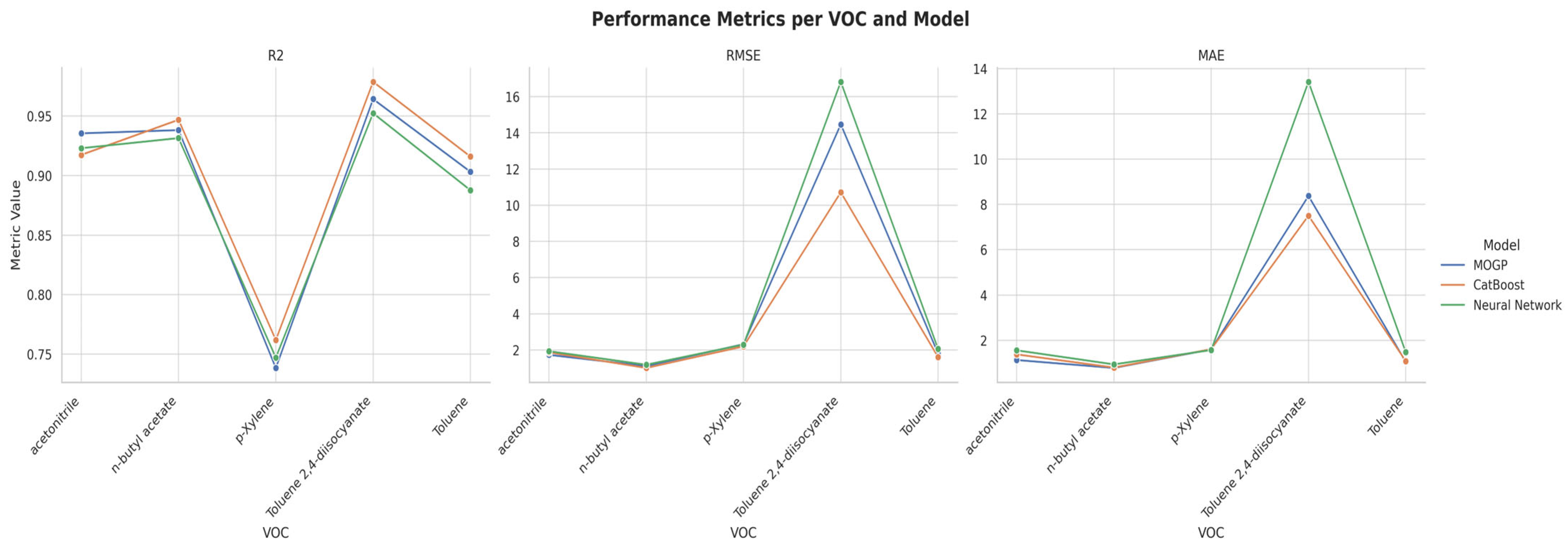
| Model | VOC | R2 | RMSE | MAE |
|---|---|---|---|---|
| MOGP | acetonitrile | 0.9355 | 1.7313 | 1.1284 |
| n-butyl acetate | 0.9382 | 1.1103 | 0.7778 | |
| p-Xylene | 0.7383 | 2.3193 | 1.5984 | |
| Toluene 2,4-diisocyanate | 0.9643 | 14.4662 | 8.3748 | |
| Toluene | 0.9032 | 1.805 | 1.0428 | |
| Average | 0.8959 | 4.2864 | 2.5844 | |
| CatBoost | acetonitrile | 0.9174 | 1.87 | 1.3776 |
| n-butyl acetate | 0.9469 | 1.0066 | 0.7956 | |
| p-Xylene | 0.7618 | 2.1983 | 1.6079 | |
| Toluene 2,4-diisocyanate | 0.9788 | 10.7132 | 7.5046 | |
| Toluene | 0.916 | 1.606 | 1.0772 | |
| Average | 0.9042 | 3.4788 | 2.4726 | |
| Neural Network | acetonitrile | 0.923 | 1.9324 | 1.5573 |
| n-butyl acetate | 0.9315 | 1.1845 | 0.9353 | |
| p-Xylene | 0.747 | 2.297 | 1.5694 | |
| Toluene 2,4-diisocyanate | 0.9524 | 16.8162 | 13.4165 | |
| Toluene | 0.8877 | 2.0589 | 1.4734 | |
| Average | 0.8883 | 4.8578 | 3.7904 |
| Age | Gender | Smoking Status | ||||||||||
|---|---|---|---|---|---|---|---|---|---|---|---|---|
| ≤15 | >15 | Male | Female | Non-Smoker | Smoker | |||||||
| VOC | Mean | Std | Mean | Std | Mean | Std | Mean | Std | Mean | Std | Mean | Std |
| acetonitrile | 48.74 | 1.24 | 61.18 | 3.36 | 56.74 | 7.07 | 58.51 | 1.82 | 55.14 | 6.19 | 63.24 | 2.49 |
| n-butyl acetate | 32.37 | 0.67 | 40.46 | 2.42 | 37.65 | 4.71 | 38.33 | 0.92 | 36.37 | 3.91 | 42.35 | 1.49 |
| Toluene | 76.27 | 0.972 | 84.86 | 5.25 | 82.45 | 6.39 | 79.73 | 0.80 | 79.65 | 4.10 | 89.71 | 4.23 |
| p-Xylene | 62.16 | 1.81 | 68.76 | 2.74 | 66.60 | 4.29 | 66.34 | 1.69 | 65.19 | 3.35 | 71.07 | 2.07 |
| Toluene 2 4-diisocyanate | 127.14 | 7.53 | 274.06 | 37.36 | 222.34 | 82.66 | 238.86 | 16.61 | 199.56 | 67.75 | 308.97 | 21.22 |
Disclaimer/Publisher’s Note: The statements, opinions and data contained in all publications are solely those of the individual author(s) and contributor(s) and not of MDPI and/or the editor(s). MDPI and/or the editor(s) disclaim responsibility for any injury to people or property resulting from any ideas, methods, instructions or products referred to in the content. |
© 2025 by the authors. Licensee MDPI, Basel, Switzerland. This article is an open access article distributed under the terms and conditions of the Creative Commons Attribution (CC BY) license (https://creativecommons.org/licenses/by/4.0/).
Share and Cite
Eid, A.; Jodeh, S.; Hanbali, G.; Hawawreh, M.; Chakir, A.; Roth, E. Multi-Output Machine-Learning Prediction of Volatile Organic Compounds (VOCs): Learning from Co-Emitted VOCs. Environments 2025, 12, 216. https://doi.org/10.3390/environments12070216
Eid A, Jodeh S, Hanbali G, Hawawreh M, Chakir A, Roth E. Multi-Output Machine-Learning Prediction of Volatile Organic Compounds (VOCs): Learning from Co-Emitted VOCs. Environments. 2025; 12(7):216. https://doi.org/10.3390/environments12070216
Chicago/Turabian StyleEid, Abdelrahman, Shehdeh Jodeh, Ghadir Hanbali, Mohammad Hawawreh, Abdelkhaleq Chakir, and Estelle Roth. 2025. "Multi-Output Machine-Learning Prediction of Volatile Organic Compounds (VOCs): Learning from Co-Emitted VOCs" Environments 12, no. 7: 216. https://doi.org/10.3390/environments12070216
APA StyleEid, A., Jodeh, S., Hanbali, G., Hawawreh, M., Chakir, A., & Roth, E. (2025). Multi-Output Machine-Learning Prediction of Volatile Organic Compounds (VOCs): Learning from Co-Emitted VOCs. Environments, 12(7), 216. https://doi.org/10.3390/environments12070216