

Modeling Air Pollution in Metropolitan Lima: A Statistical and Artificial Neural Network Approach

 ,
, 
Abstract
1. Introduction
2. Methodology
2.1. Box–Jenkins Models
2.2. Exponential Smoothing Method
2.3. Neural Network Autoregression
2.4. Multi-Layer Perceptron
2.5. Long Short-Term Memory
2.6. Dynamic Linear Model
3. Results
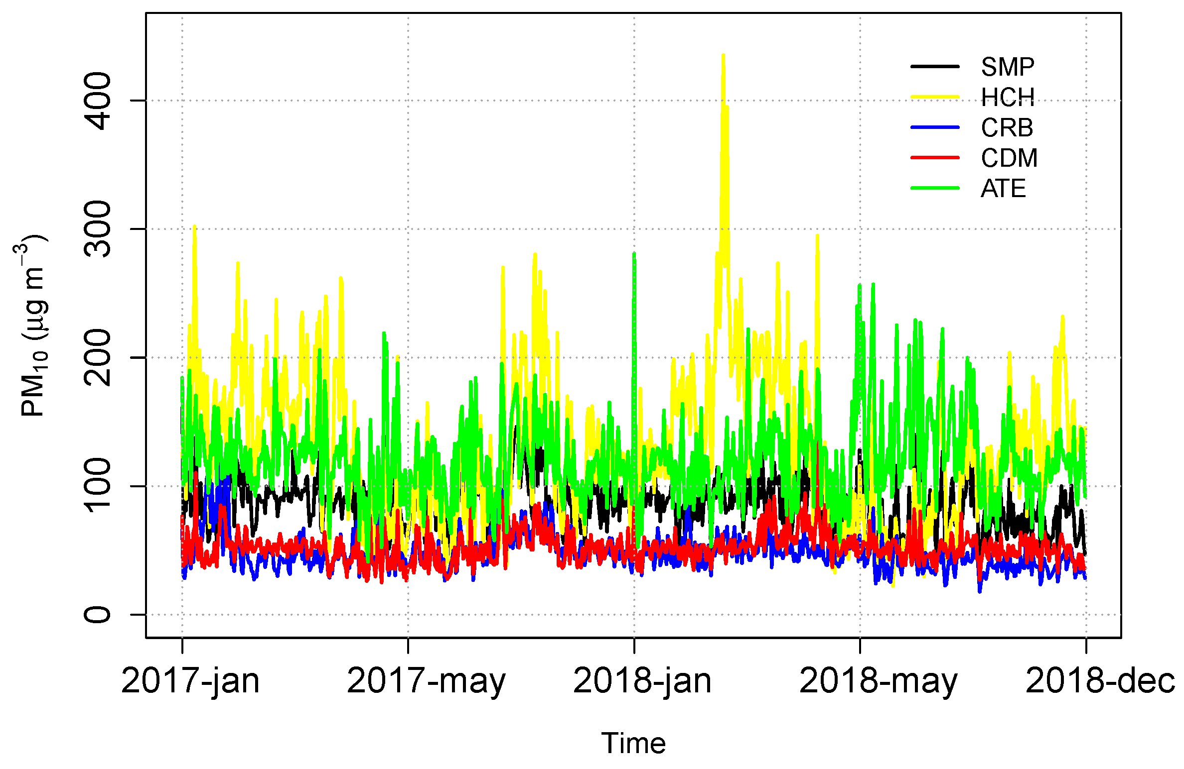
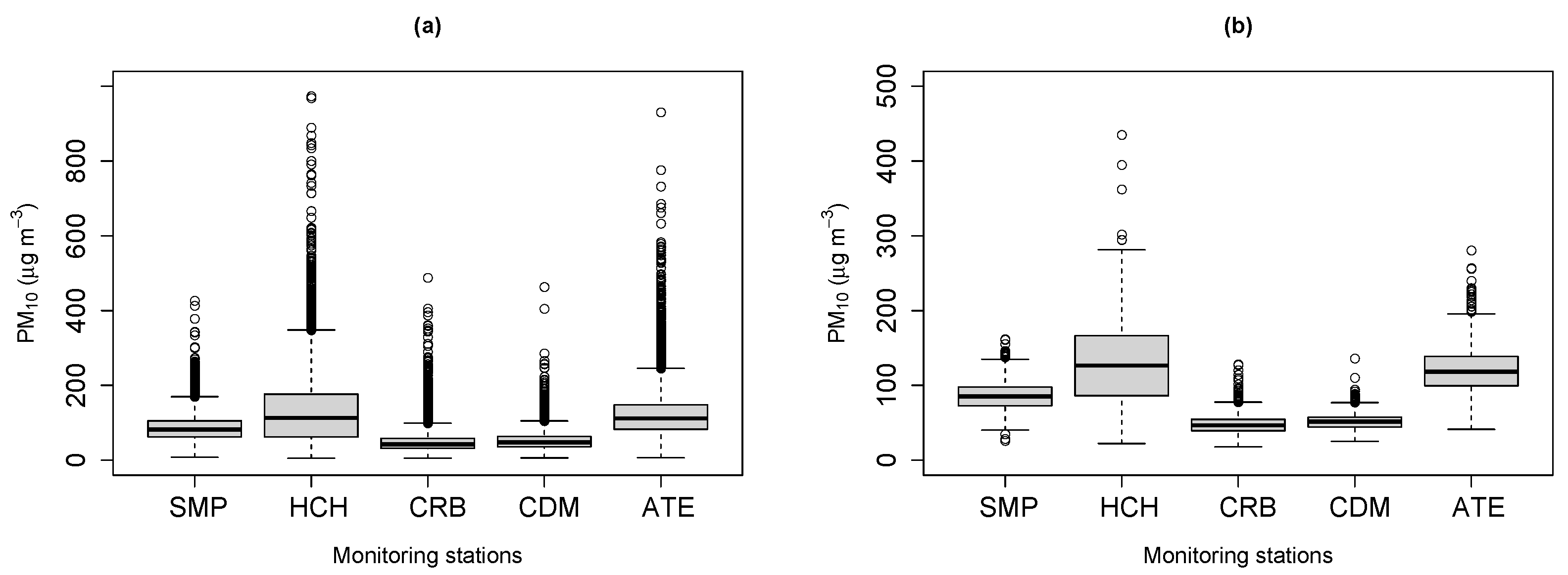
3.1. Exploratory Analysis
3.2. Model Performance Evaluation for PM10 Forecasting in Lima
3.3. Limitations and Future Work
4. Conclusions
Author Contributions
Funding
Institutional Review Board Statement
Informed Consent Statement
Data Availability Statement
Conflicts of Interest
References
- Hoek, G.; Krishnan, R.M.; Beelen, R.; Peters, A.; Ostro, B.; Brunekreef, B.; Kaufman, J.D. Long-term air pollution exposure and cardio-respiratory mortality: A review. Environ. Health 2013, 12, 43. [Google Scholar] [CrossRef] [PubMed]
- Chen, J.; Hoek, G. Long-term exposure to PM and all-cause and cause-specific mortality: A systematic review and meta-analysis. Environ. Int. 2020, 143, 105974. [Google Scholar] [CrossRef] [PubMed]
- Sánchez-Balseca, J.; Pérez-Foguet, A. Spatio-temporal air pollution modelling using a compositional approach. Heliyon 2020, 6, e04794. [Google Scholar] [CrossRef]
- Mahmud, H.; Shobnom, K.; Ali, M.R.; Muntakim, N.; Kulsum, U.; Baroi, D.S.; Ahmed, Z.; Rahman, M.M.; Hassan, M.Z. Micro-environmental dynamics of particulate (PM2.5 and PM10) air pollution in Rajshahi City: A spatiotemporal analysis. Manag. Environ. Qual. Int. J. 2024, 35, 1773–1797. [Google Scholar] [CrossRef]
- Akdi, Y.; Gölveren, E.; Ünlü, K.D.; Yücel, M.E. Modeling and forecasting of monthly PM2.5 emission of Paris by periodogram-based time series methodology. Environ. Monit. Assess. 2021, 193, 622. [Google Scholar] [CrossRef]
- Leng, S.; Gao, X.; Pei, T.; Zhang, G.; Chen, L.; Chen, X.; He, C.; He, D.; Li, X.; Lin, C.; et al. Tempo-Spatial Processes and Modelling of Environmental Pollutants. In The Geographical Sciences During 1986–2015: From the Classics to the Frontiers; Springer: Singapore, 2017; pp. 367–390. [Google Scholar]
- Thompson, J.E. Airborne particulate matter: Human exposure and health effects. J. Occup. Environ. Med. 2018, 60, 392–423. [Google Scholar] [CrossRef]
- Cekim, H.O. Forecasting PM10 concentrations using time series models: A case of the most polluted cities in Turkey. Environ. Sci. Pollut. Res. 2020, 27, 25612–25624. [Google Scholar] [CrossRef] [PubMed]
- Performance Analysis of Machine Learning Singular Spectrum Analysis for Forecasting Air Contamination. In Proceedings of the 2023 International Conference on System, Computation, Automation and Networking (ICSCAN), Puducherry, India, 17–18 November 2023. [CrossRef]
- Kumar, U. An integrated SSA-ARIMA approach to make multiple day ahead forecasts for the daily maximum ambient O3 concentration. Aerosol Air Qual. Res. 2015, 15, 208–219. [Google Scholar] [CrossRef]
- Cai, J.; Gu, C.; Fang, K.; Wang, L.; Lv, M. Long-term PM2.5 Concentration Prediction Using Hybrid Deep Learning Model. In Proceedings of the 2023 4th International Conference on Computers and Artificial Intelligence Technology (CAIT), Macau, Macao, 13–15 December 2023. [Google Scholar] [CrossRef]
- Bodor, Z.; Bodor, K.; Keresztesi, Á.; Szép, R. Major air pollutants seasonal variation analysis and long-range transport of PM10 in an urban environment with specific climate condition in Transylvania (Romania). Environ. Sci. Pollut. Res. 2020, 27, 38181–38199. [Google Scholar] [CrossRef]
- Shikhovtsev, M.Y.; Obolkin, V.; Khodzher, T.; Molozhnikova, Y.V. Variability of the ground concentration of particulate matter PM1–PM10 in the air basin of the Southern Baikal Region. Atmos. Ocean. Opt. 2023, 36, 655–662. [Google Scholar] [CrossRef]
- Li, B.; Rodell, M. Spatial variability and its scale dependency of observed and modeled soil moisture over different climate regions. Hydrol. Earth Syst. Sci. 2013, 17, 1177–1188. [Google Scholar] [CrossRef]
- Rojas, I.; Valenzuela, O.; Rojas, F.; Guillen, A.; Herrera, L.; Pomares, H.; Marquez, L.; Pasadas, M. Soft-computing techniques and ARMA model for time series prediction. Neurocomputing 2008, 71, 519–537. [Google Scholar] [CrossRef]
- Aguilar, S.; Castro Souza, R.; Pessanha, J.F.; Cyrino Oliveira, F.L. Hybrid methodology for modeling short-term wind power generation using conditional Kernel density estimation and singular spectrum analysis. Dyna 2017, 84, 145–154. [Google Scholar] [CrossRef]
- López-Gonzales, J.L.; Salas, R.; Velandia, D.; Canas Rodrigues, P. Air quality prediction based on singular spectrum analysis and artificial neural networks. Entropy 2024, 26, 1062. [Google Scholar] [CrossRef]
- Espinosa, F.; Bartolomé, A.B.; Hernández, P.V.; Rodriguez-Sanchez, M. Contribution of singular spectral analysis to forecasting and anomalies detection of indoors air quality. Sensors 2022, 22, 3054. [Google Scholar] [CrossRef]
- Espinoza Guillen, J.A. Evaluación Espacial y Temporal del Material Particulado PM10 y PM2.5 en Lima Metropolitana para el Periodo 2015–2017. Bachelor’s Thesis, Universidad Nacional Agraria La Molina, Lima, Peru, 2018. [Google Scholar]
- Silva, J.; Rojas, J.; Norabuena, M.; Molina, C.; Toro, R.A.; Leiva-Guzmán, M.A. Particulate matter levels in a South American megacity: The metropolitan area of Lima-Callao, Peru. Environ. Monit. Assess. 2017, 189, 635. [Google Scholar] [CrossRef]
- Aceves-Fernandez, M.A.; Pedraza-Ortega, J.C.; Sotomayor-Olmedo, A.; Ramos-Arreguín, J.M.; Vargas-Soto, J.E.; Tovar-Arriaga, S. Analysis of key features of non-linear behaviour using recurrence quantification. Case study: Urban Airborne pollution at Mexico city. Environ. Model. Assess. 2014, 19, 139–152. [Google Scholar] [CrossRef]
- Box, G.; Jenkins, G. Time Series Analysis: Forecasting and Control; Holden-Day series in time series analysis and digital processing; Holden-Day: Clarendon, Australia, 1970. [Google Scholar]
- Hyndman, R.J.; Khandakar, Y. Automatic time series forecasting: The forecast package for R. J. Stat. Softw. 2008, 27, 1–22. [Google Scholar] [CrossRef]
- Brown, R.G. Statistical Forecasting for Inventory Control; McGraw-Hill: New York, NY, USA, 1959. [Google Scholar]
- Holt, C.C. Forecasting seasonals and trends by exponentially weighted moving averages. Int. J. Forecast. 2004, 20, 5–10. [Google Scholar] [CrossRef]
- Winters, P.R. Forecasting sales by exponentially weighted moving averages. Manag. Sci. 1960, 6, 324–342. [Google Scholar] [CrossRef]
- Hyndman, R.; Athanasopoulos, G. Forecasting: Principles and Practice, 2nd ed.; OTexts: Melbourne, Australia, 2018. [Google Scholar]
- Hyndman, R.; Koehler, A.; Ord, K.; Snyder, R. Forecasting with Exponential Smoothing. The State Space Approach; Springer: Berlin/Heidelberg, Germany, 2008. [Google Scholar] [CrossRef]
- Zhang, G.P.; Patuwo, B.E.; Hu, M.Y. Forecasting with artificial neural networks: The state of the art. Int. J. Forecast. 1998, 14, 35–62. [Google Scholar] [CrossRef]
- Crone, S.F.; Kourentzes, N. Feature selection for time series prediction—A combined filter and wrapper approach for neural networks. Neurocomputing 2010, 73, 1923–1936. [Google Scholar] [CrossRef]
- Goodfellow, I.; Bengio, Y.; Courville, A. Deep Learning; MIT Press: Cambridge, MA, USA, 2016. [Google Scholar]
- Glorot, X.; Bordes, A.; Bengio, Y. Deep sparse rectifier neural networks. In Proceedings of the Fourteenth International Conference on Artificial Intelligence and Statistics, Fort Lauderdale, FL, USA, 11–13 April 2011; Volume 15, pp. 315–323. [Google Scholar]
- Hornik, K.; Stinchcombe, M.; White, H. Multilayer feedforward networks are universal approximators. Neural Netw. 1989, 2, 359–366. [Google Scholar] [CrossRef]
- Hochreiter, S.; Schmidhuber, J. Long short-term memory. Neural Comput. 1997, 9, 1735–1780. [Google Scholar] [CrossRef]
- Gers, F.A.; Schmidhuber, J.; Cummins, F. Learning to forget: Continual prediction with LSTM. Neural Comput. 2002, 12, 2451–2471. [Google Scholar] [CrossRef] [PubMed]
- Greff, K.; Srivastava, R.K.; Koutník, J.; Steunebrink, B.R.; Schmidhuber, J. LSTM: A search space odyssey. IEEE Trans. Neural Networks Learn. Syst. 2017, 28, 2222–2232. [Google Scholar] [CrossRef]
- West, M.; Harrison, J. Bayesian Forecasting and Dynamic Models, 2nd ed.; Springer: Berlin/Heidelberg, Germany, 1997. [Google Scholar]
- Petris, G. An R Package for Dynamic Linear Models. J. Stat. Softw. 2010, 36, 1–16. [Google Scholar] [CrossRef]
- Gonzales, S.M.; Iftikhar, H.; López-Gonzales, J.L. Analysis and forecasting of electricity prices using an improved time series ensemble approach: An application to the Peruvian electricity market. Aims Math 2024, 9, 21952–21971. [Google Scholar] [CrossRef]
- Iftikhar, H.; Gonzales, S.M.; Zywiołek, J.; López-Gonzales, J.L. Electricity demand forecasting using a novel time series ensemble technique. IEEE Access 2024, 12, 88963–88975. [Google Scholar] [CrossRef]
- da Silva, K.L.S.; López-Gonzales, J.L.; Turpo-Chaparro, J.E.; Tocto-Cano, E.; Rodrigues, P.C. Spatio-temporal visualization and forecasting of PM10 in the Brazilian state of Minas Gerais. Sci. Rep. 2023, 13, 3269. [Google Scholar] [CrossRef]
- Cruz, A.R.H.D.L.; Ayuque, R.F.O.; Cruz, R.W.H.D.L.; Lopez-Gonzales, J.L.; Gioda, A. Air quality biomonitoring of trace elements in the metropolitan area of Huancayo, Peru using transplanted Tillandsia capillaris as a biomonitor. An. Acad. Bras. Ciências 2020, 92, e20180813. [Google Scholar] [CrossRef] [PubMed]


| Measures | SMP | HCH | CRB | CDM | ATE |
|---|---|---|---|---|---|
| Minimum | 26.01 | 22.22 | 17.84 | 25.12 | 41.26 |
| 1st Qu. | 72.89 | 86.21 | 39.38 | 44.35 | 99.59 |
| Median | 85.29 | 126.61 | 46.40 | 51.46 | 118.19 |
| Mean | 86.05 | 130.03 | 48.69 | 52.30 | 121.56 |
| 3rd Qu. | 97.69 | 166.56 | 54.63 | 57.51 | 138.72 |
| Maximum | 161.97 | 435.15 | 128.44 | 136.16 | 280.72 |
| Standard deviation | 20.88 | 58.63 | 14.50 | 12.25 | 33.29 |
| Metric | Sets | ETS | ARIMA | TBATS | NNAR | MLP | DLM | SSA | NAÏVE | LSTM |
|---|---|---|---|---|---|---|---|---|---|---|
| RMSE | 1 | 8.073 | 12.131 | 9.991 | 8.804 | 10.914 | 39.730 | 8.081 | 15.614 | 9.683 |
| 2 | 11.862 | 13.691 | 12.284 | 13.873 | 13.460 | 41.701 | 13.232 | 12.470 | 12.661 | |
| 3 | 15.951 | 15.123 | 14.930 | 19.771 | 17.941 | 13.320 | 18.412 | 15.572 | 18.391 | |
| 4 | 18.141 | 16.362 | 16.954 | 22.173 | 20.874 | 13.701 | 21.701 | 17.232 | 20.704 | |
| 5 | 20.410 | 15.962 | 17.771 | 25.403 | 23.171 | 38.762 | 23.761 | 22.962 | 24.494 | |
| 6 | 24.390 | 15.511 | 18.872 | 28.314 | 26.591 | 82.103 | 24.872 | 37.531 | 25.174 | |
| 7 | 23.804 | 15.341 | 18.063 | 26.942 | 24.394 | 15.911 | 25.822 | 21.823 | 21.444 | |
| 8 | 21.773 | 15.001 | 17.473 | 24.881 | 23.640 | 27.771 | 26.223 | 15.383 | 24.580 | |
| 9 | 16.913 | 12.884 | 14.763 | 18.961 | 20.190 | 66.444 | 25.323 | 10.751 | 24.394 | |
| 10 | 13.833 | 14.052 | 15.020 | 14.691 | 20.084 | 48.243 | 20.801 | 14.054 | 23.583 | |
| Average | 17.514 | 14.603 | 15.611 | 20.383 | 20.120 | 38.774 | 20.823 | 18.343 | 20.511 | |
| sMAPE (%) | 1 | 1.871 | 2.801 | 2.030 | 2.193 | 2.954 | 9.184 | 1.853 | 4.150 | 2.621 |
| 2 | 2.714 | 3.643 | 2.951 | 3.094 | 3.091 | 17.170 | 3.113 | 2.981 | 2.964 | |
| 3 | 4.130 | 4.213 | 3.981 | 4.950 | 4.444 | 3.691 | 4.633 | 4.080 | 4.701 | |
| 4 | 5.240 | 5.041 | 5.034 | 6.260 | 5.691 | 4.194 | 5.833 | 5.121 | 5.611 | |
| 5 | 6.234 | 5.081 | 5.543 | 7.573 | 6.901 | 10.322 | 7.032 | 6.890 | 7.292 | |
| 6 | 7.560 | 5.022 | 6.091 | 8.863 | 8.363 | 18.440 | 7.621 | 11.152 | 7.802 | |
| 7 | 7.484 | 5.044 | 5.731 | 8.440 | 7.603 | 4.954 | 8.011 | 6.853 | 6.734 | |
| 8 | 6.921 | 4.982 | 5.652 | 8.011 | 7.580 | 10.091 | 8.001 | 5.092 | 7.804 | |
| 9 | 5.564 | 4.423 | 4.981 | 6.232 | 6.512 | 33.884 | 7.920 | 3.071 | 7.743 | |
| 10 | 4.732 | 4.554 | 4.910 | 4.891 | 6.274 | 30.032 | 6.742 | 4.474 | 7.473 | |
| Average | 5.242 | 4.480 | 4.693 | 6.054 | 5.942 | 14.190 | 6.071 | 5.382 | 6.074 |
| Metric | Sets | ETS | ARIMA | TBATS | NNAR | MLP | DLM | SSA | NAÏVE | LSTM |
|---|---|---|---|---|---|---|---|---|---|---|
| RMSE | 1 | 75.224 | 41.614 | 37.843 | 44.831 | 44.084 | 41.332 | 47.854 | 56.384 | 21.922 |
| 2 | 61.504 | 42.791 | 39.084 | 46.531 | 40.504 | 62.163 | 58.983 | 36.132 | 21.102 | |
| 3 | 43.873 | 37.374 | 34.541 | 36.793 | 30.843 | 82.413 | 57.581 | 22.631 | 20.662 | |
| 4 | 19.683 | 23.664 | 20.934 | 36.603 | 15.354 | 167.442 | 43.674 | 33.824 | 15.742 | |
| 5 | 24.712 | 26.954 | 25.173 | 41.804 | 17.403 | 18.761 | 31.742 | 16.421 | 20.302 | |
| 6 | 24.451 | 22.964 | 22.123 | 50.734 | 16.931 | 17.262 | 18.214 | 17.161 | 16.104 | |
| 7 | 42.721 | 30.093 | 28.904 | 49.704 | 21.153 | 98.882 | 14.402 | 32.391 | 17.152 | |
| 8 | 53.264 | 33.733 | 32.884 | 65.842 | 29.553 | 77.753 | 11.163 | 39.013 | 17.994 | |
| 9 | 26.482 | 22.543 | 21.043 | 23.404 | 17.013 | 107.383 | 9.194 | 12.692 | 8.743 | |
| 10 | 25.843 | 24.072 | 23.392 | 36.624 | 18.894 | 11.324 | 13.321 | 12.403 | 11.953 | |
| Average | 39.773 | 30.582 | 28.594 | 43.281 | 25.173 | 68.472 | 30.613 | 27.902 | 17.161 | |
| sMAPE (%) | 1 | 9.963 | 5.761 | 5.214 | 6.123 | 5.942 | 5.404 | 6.564 | 7.741 | 3.102 |
| 2 | 8.724 | 6.183 | 5.612 | 6.621 | 5.701 | 11.803 | 8.443 | 5.101 | 2.924 | |
| 3 | 6.453 | 5.584 | 5.121 | 5.462 | 4.513 | 19.271 | 8.374 | 3.583 | 2.944 | |
| 4 | 2.963 | 3.103 | 2.943 | 4.663 | 2.312 | 39.583 | 6.472 | 5.754 | 2.383 | |
| 5 | 3.874 | 3.932 | 3.732 | 5.614 | 2.912 | 2.981 | 4.721 | 2.334 | 2.591 | |
| 6 | 4.071 | 3.393 | 3.521 | 6.902 | 2.521 | 2.553 | 2.613 | 2.423 | 2.324 | |
| 7 | 6.451 | 4.553 | 4.513 | 7.541 | 3.394 | 12.284 | 2.354 | 5.034 | 2.302 | |
| 8 | 8.374 | 5.542 | 5.451 | 9.841 | 4.931 | 11.164 | 1.471 | 6.463 | 2.953 | |
| 9 | 3.942 | 3.604 | 3.392 | 3.463 | 2.861 | 31.184 | 1.194 | 1.982 | 1.371 | |
| 10 | 4.021 | 3.874 | 3.731 | 5.381 | 2.984 | 1.771 | 1.751 | 2.183 | 1.532 | |
| Average | 5.881 | 4.553 | 4.324 | 6.161 | 3.814 | 13.804 | 4.393 | 4.261 | 2.442 |
| ETS | ARIMA | TBATS | NNAR | MLP | DLM | SSA | NAÏVE | LSTM | ||
|---|---|---|---|---|---|---|---|---|---|---|
| RMSE | 1 | 5.614 | 5.294 | 5.302 | 7.401 | 7.904 | 20.104 | 5.671 | 9.631 | 7.751 |
| 2 | 6.302 | 6.642 | 6.504 | 7.814 | 7.574 | 40.282 | 6.641 | 8.911 | 9.224 | |
| 3 | 7.121 | 7.072 | 6.884 | 9.431 | 9.102 | 8.134 | 7.754 | 7.102 | 11.162 | |
| 4 | 7.284 | 7.042 | 6.841 | 10.421 | 9.344 | 12.491 | 7.754 | 7.521 | 12.614 | |
| 5 | 7.744 | 7.262 | 6.882 | 11.304 | 10.024 | 12.194 | 8.292 | 8.214 | 12.284 | |
| 6 | 10.312 | 8.872 | 8.574 | 13.274 | 12.654 | 38.324 | 8.861 | 16.021 | 14.074 | |
| 7 | 9.571 | 7.962 | 6.431 | 11.934 | 11.464 | 8.861 | 9.194 | 8.112 | 13.574 | |
| 8 | 9.181 | 8.192 | 7.854 | 12.114 | 11.764 | 6.972 | 9.504 | 8.042 | 15.804 | |
| 9 | 4.332 | 4.182 | 3.504 | 6.964 | 6.874 | 45.434 | 8.214 | 8.401 | 11.964 | |
| 10 | 4.384 | 5.424 | 5.094 | 9.294 | 8.764 | 11.741 | 6.934 | 5.542 | 12.574 | |
| Average | 7.181 | 6.792 | 6.384 | 9.994 | 9.544 | 20.454 | 7.884 | 8.754 | 12.104 | |
| SMAPE (%) | 1 | 2.854 | 2.134 | 2.114 | 3.864 | 4.024 | 9.374 | 2.661 | 4.741 | 3.961 |
| 2 | 2.454 | 3.444 | 3.214 | 3.314 | 3.094 | 35.394 | 2.991 | 5.264 | 4.484 | |
| 3 | 3.404 | 3.694 | 3.604 | 4.494 | 4.154 | 4.354 | 3.584 | 3.884 | 5.454 | |
| 4 | 3.534 | 3.534 | 3.484 | 5.284 | 4.624 | 5.944 | 3.654 | 3.484 | 6.284 | |
| 5 | 3.954 | 3.823 | 3.654 | 6.164 | 5.294 | 6.402 | 4.191 | 4.251 | 6.463 | |
| 6 | 5.752 | 5.042 | 4.854 | 7.543 | 7.171 | 16.314 | 4.754 | 8.874 | 7.874 | |
| 7 | 5.334 | 4.322 | 3.604 | 6.704 | 6.421 | 5.542 | 4.953 | 4.351 | 7.653 | |
| 8 | 5.261 | 4.641 | 4.314 | 7.132 | 6.954 | 3.851 | 5.054 | 4.501 | 8.924 | |
| 9 | 2.444 | 2.222 | 1.974 | 3.941 | 3.844 | 39.854 | 4.544 | 5.741 | 6.891 | |
| 10 | 2.604 | 3.062 | 2.904 | 5.002 | 4.391 | 9.141 | 3.964 | 3.291 | 7.221 | |
| Average | 3.764 | 3.591 | 3.374 | 5.341 | 4.994 | 13.614 | 4.031 | 4.841 | 6.523 |
| ETS | ARIMA | TBATS | NNAR | MLP | DLM | SSA | NAÏVE | LSTM | ||
|---|---|---|---|---|---|---|---|---|---|---|
| RMSE | 1 | 13.831 | 13.782 | 14.802 | 12.973 | 12.321 | 15.751 | 15.474 | 12.301 | 12.622 |
| 2 | 12.881 | 13.231 | 15.252 | 12.763 | 12.612 | 31.471 | 15.642 | 14.322 | 12.992 | |
| 3 | 19.191 | 17.412 | 16.023 | 18.601 | 16.634 | 29.031 | 15.974 | 17.692 | 16.041 | |
| 4 | 25.511 | 22.161 | 19.132 | 23.151 | 21.721 | 32.961 | 17.302 | 23.602 | 19.822 | |
| 5 | 20.733 | 18.922 | 18.991 | 19.453 | 20.123 | 60.593 | 16.252 | 20.951 | 18.602 | |
| 6 | 21.412 | 19.352 | 18.251 | 19.771 | 19.973 | 25.042 | 15.791 | 19.183 | 21.363 | |
| 7 | 22.854 | 22.073 | 21.512 | 22.803 | 21.896 | 27.723 | 20.553 | 22.222 | 23.534 | |
| 8 | 26.202 | 23.584 | 22.763 | 23.602 | 26.193 | 101.282 | 21.364 | 37.993 | 21.614 | |
| 9 | 23.114 | 20.401 | 20.432 | 19.653 | 21.254 | 62.064 | 20.903 | 21.144 | 21.902 | |
| 10 | 20.712 | 19.264 | 19.779 | 19.883 | 19.585 | 107.774 | 21.863 | 31.865 | 21.674 | |
| Average | 20.643 | 19.024 | 18.693 | 19.265 | 19.235 | 49.375 | 18.114 | 22.124 | 19.013 | |
| SMAPE (%) | 1 | 2.403 | 2.262 | 2.324 | 2.083 | 1.883 | 2.422 | 2.172 | 1.873 | 1.952 |
| 2 | 2.135 | 2.064 | 2.393 | 1.965 | 2.013 | 6.143 | 2.197 | 2.164 | 1.902 | |
| 3 | 3.342 | 3.042 | 2.553 | 3.086 | 2.713 | 4.674 | 2.485 | 3.052 | 2.594 | |
| 4 | 4.802 | 4.193 | 3.373 | 4.314 | 4.025 | 5.893 | 3.091 | 4.506 | 3.484 | |
| 5 | 3.403 | 3.104 | 3.422 | 3.213 | 3.432 | 17.782 | 2.903 | 4.113 | 3.004 | |
| 6 | 3.812 | 3.401 | 3.104 | 3.564 | 3.562 | 4.613 | 2.682 | 3.324 | 3.903 | |
| 7 | 4.362 | 4.123 | 3.873 | 4.214 | 4.083 | 5.162 | 3.613 | 4.146 | 4.553 | |
| 8 | 4.864 | 4.521 | 4.424 | 4.613 | 5.013 | 15.074 | 3.736 | 6.443 | 4.071 | |
| 9 | 4.423 | 3.723 | 3.792 | 3.674 | 4.093 | 14.294 | 3.885 | 3.944 | 4.092 | |
| 10 | 3.774 | 3.602 | 3.673 | 3.724 | 3.564 | 33.742 | 4.013 | 5.803 | 3.963 | |
| Average | 3.733 | 3.404 | 3.295 | 3.443 | 3.441 | 10.983 | 3.076 | 3.933 | 3.352 |
Disclaimer/Publisher’s Note: The statements, opinions and data contained in all publications are solely those of the individual author(s) and contributor(s) and not of MDPI and/or the editor(s). MDPI and/or the editor(s) disclaim responsibility for any injury to people or property resulting from any ideas, methods, instructions or products referred to in the content. |
© 2025 by the authors. Licensee MDPI, Basel, Switzerland. This article is an open access article distributed under the terms and conditions of the Creative Commons Attribution (CC BY) license (https://creativecommons.org/licenses/by/4.0/).
Share and Cite
Solis Teran, M.A.; Leite Coelho da Silva, F.; Torres Armas, E.A.; Carbo-Bustinza, N.; López-Gonzales, J.L. Modeling Air Pollution in Metropolitan Lima: A Statistical and Artificial Neural Network Approach. Environments 2025, 12, 196. https://doi.org/10.3390/environments12060196
Solis Teran MA, Leite Coelho da Silva F, Torres Armas EA, Carbo-Bustinza N, López-Gonzales JL. Modeling Air Pollution in Metropolitan Lima: A Statistical and Artificial Neural Network Approach. Environments. 2025; 12(6):196. https://doi.org/10.3390/environments12060196
Chicago/Turabian StyleSolis Teran, Miguel Angel, Felipe Leite Coelho da Silva, Elías A. Torres Armas, Natalí Carbo-Bustinza, and Javier Linkolk López-Gonzales. 2025. "Modeling Air Pollution in Metropolitan Lima: A Statistical and Artificial Neural Network Approach" Environments 12, no. 6: 196. https://doi.org/10.3390/environments12060196
APA StyleSolis Teran, M. A., Leite Coelho da Silva, F., Torres Armas, E. A., Carbo-Bustinza, N., & López-Gonzales, J. L. (2025). Modeling Air Pollution in Metropolitan Lima: A Statistical and Artificial Neural Network Approach. Environments, 12(6), 196. https://doi.org/10.3390/environments12060196