Urban Source Apportionment of Potentially Toxic Elements in Thessaloniki Using Syntrichia Moss Biomonitoring and PMF Modeling

Abstract

Urban air pollution from potentially toxic elements (PTEs) presents a critical threat to public health and environmental sustainability. The current study employed Syntrichia moss in a passive biomonitoring capacity to ascertain the levels of atmospheric PTE pollution in Thessaloniki, Greece. A comprehensive collection of 192 moss samples was undertaken at 16 urban sampling points over the March–July 2024 period. Concentrations of 21 PTEs were quantified using ICP-MS, and contamination levels were assessed through contamination factor (CF), enrichment factor (EF), and pollution load index (PLI). Positive matrix factorization (PMF) modeling and multivariate statistical analyses were used to identify pollution sources and spatiotemporal variations. Results revealed persistent hotspots with significant anthropogenic enrichments of elements, such as Fe, Mn, Sn in industrial zones and Tl, Ce, Pt in traffic corridors. PMF modeling attributed 48% of the measured PTE variance to traffic-related sources, 35% to industrial sources, and 17% to crustal material. Seasonal transitions showed a significant 3.5-fold increase in Tl during summer, indicating elevated traffic-related emissions. This integrated multi-index and source apportionment framework demonstrates the efficacy of Syntrichia moss for high-resolution urban air quality assessment. The approach offers a cost-effective, scalable, and environmentally friendly tool to support EU-aligned air quality management strategies.

1. Introduction

Air pollution contributes to severe health issues, including respiratory and cardiovascular diseases and causes millions of premature deaths annually. Urban areas, with high population densities and concentrated industrial activities, are particularly vulnerable to elevated levels of air pollutants from anthropogenic sources like traffic, industry, and heating [1,2]. Among various pollutants, potentially toxic elements (PTEs), including both macro-elements at high concentrations, and metal and metalloid elements, pose significant concerns due to their toxicity and bioaccumulation potential [3].

Among the various pollutants, PTEs have gathered significant attention due to their dual nature. Macro elements, such as calcium, phosphorus, sodium, potassium, etc., play vital roles in biological and ecological processes. However, their excessive accumulation can disrupt ecosystem balance and harm human health [4,5,6,7,8,9]. Trace elements are of particular concern due to their toxicity, even at low concentrations, and their ability to bioaccumulate in biological tissues over time [10].

Traditional air quality monitoring networks, reliant on sophisticated instrumentation, provide valuable real-time data on pollutant concentrations at specific locations. Traditional monitoring networks, though valuable, face limitations in cost and spatial coverage. Biomonitoring using mosses like Syntrichia offers a cost-effective alternative. These organisms efficiently accumulate elements via atmospheric deposition and direct nutrient uptake [11]. Their efficacy has been demonstrated in urban and desert environments, highlighting their utility in pollution assessment [12].

Multiple factors contribute to Thessaloniki’s air quality issues, including its challenging topography, large population, industrial presence, and high traffic volumes—challenges typical of Greece’s second-largest urban center. While the city has established air quality monitoring networks, these systems primarily measure criteria pollutants. In addition to these criteria pollutants, EU directives (e.g., 2008/50/EC and 2004/107/EC) also mandate the monitoring of specific hazardous substances in ambient air, including certain heavy metals and metalloids, to assess compliance with health-based air quality standards. In response to the persistent air pollution, particularly concerning PM10 levels in Thessaloniki, the European Commission escalated the issue in December 2020 by initiating legal proceedings against Greece in the European Court of Justice [13]. Thus, Thessaloniki’s unique geographical and meteorological conditions, characterized by frequent temperature inversions and limited wind dispersion, exacerbate air pollution issues, making it a critical area for in-depth air quality studies.

Moss biomonitoring studies face limitations such as low spatial resolution, inconsistent methodologies, inadequate source attribution, and limited temporal resolution, impacting their reliability [14]. Sparse sampling networks can overlook pollution hotspots, reducing the accuracy of air quality assessments [15]. Variability in moss species, exposure periods, and analytical techniques hinders cross-study comparisons [16]. Additionally, traditional contamination indices lack precise source differentiation, often misattributing pollution origins [17]. Seasonal monitoring captures short-term pollution fluctuations, addressing limitations in temporal resolution [18]. Empirical baseline corrections mitigate overestimation of geogenic contributions, refining source attribution accuracy [19]. This comprehensive approach enhances the applicability of moss biomonitoring for high-resolution urban air quality assessment.

Building on previous studies that have validated Syntrichia as a reliable bioindicator [20,21], this study investigated the spatiotemporal dynamics of PTE accumulation in Syntrichia moss, reflecting airborne PTE levels in Thessaloniki. As a city under European Union legal scrutiny for persistent PM10 violations, understanding the primary sources and extent of its air pollution is critical. The present study achieved this through a novel integration of high-resolution Syntrichia moss biomonitoring, multi-index analysis, and positive matrix factorization (PMF) modeling. The core investigation centers on understanding how spatial and temporal variations in PTE concentrations, accumulated within the moss tissues, reflect the contributions of both geogenic and anthropogenic emission sources across the urban landscape. The research further explores the influence of seasonal changes and meteorological factors on PTE deposition patterns. By combining these approaches, this study provides a comprehensive assessment of air quality, establishes a pre-metro baseline, and evaluates air pollution dynamics. Specific objectives guiding the research include the quantification of PTE levels, mapping of PTE accumulation patterns in moss, assessment of seasonal variations, distinction between natural and human-caused contributions, and integration of analytical techniques for source identification.

2. Materials and Methods

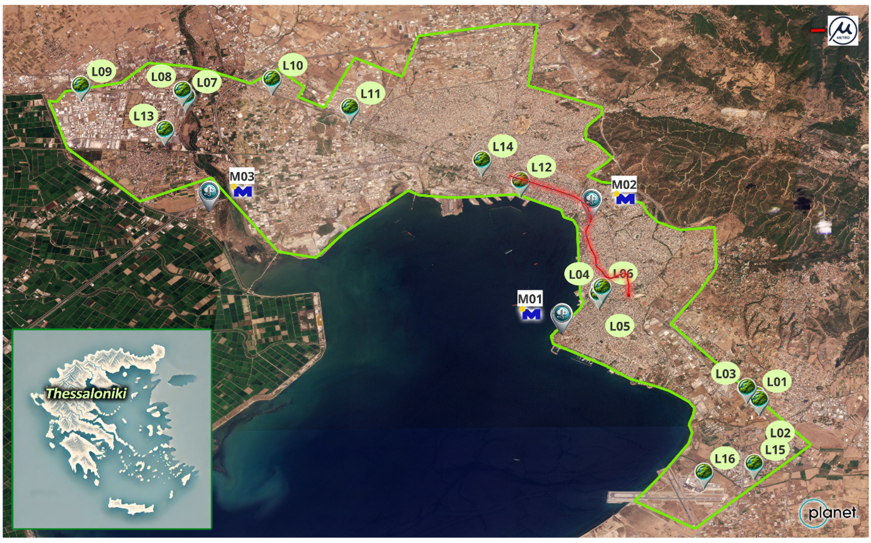
2.1. Syntrichia Moss Collection Strategy

We utilized Syntrichia as the bioindicator for this research, leveraging its known attributes of urban adaptability, stressor tolerance, and efficient PTE sequestration. To effectively assess PTE distribution, sampling locations were selected to represent a spectrum of land-use types, which allowed for mapping element variability and pinpointing potential contamination foci. The sampling locations were strategically chosen to be representative of the overall urban area of Thessaloniki, encompassing a diverse range of pollution sources, including industrial emissions, high-traffic roadways, residential areas, and the airport vicinity (

Table 1. Site characterization for moss sampling locations in the urban area of Thessaloniki.

Site Type	Selection Criteria	Locations
Motorway	Chosen to assess the effects of traffic-related pollutant emitted along the heavily trafficked roadway. High traffic density involving passenger and commercial vehicles contributes to microelement deposition from vehicle wear and emissions.	L01, L02, L03
Airport Surroundings	Aircraft emissions contribute significantly to local air quality through the deposition of elements, which can be linked to aviation fuel and exhaust. This provides insights into localized deposition patterns related to aviation activities.	L15, L16
City Center	This zone reflects the complexity of central urban environments, where elevated population density and diverse land uses contribute to a multifactorial pollution profile. The interplay of vehicular traffic, commercial operations, and residential energy use in this area is expected to significantly influence the spatial heterogeneity of PTE concentrations.	L04, L05, L06, L11, L12, L14
Industrial Zone	This area includes industries such as chemical manufacturing, metal processing, construction materials, automotive and machinery, textile and plastic production, etc., it is a key hotspot for pollution assessments (Sindos Industrial Area)	L07, L08, L09, L13
Road Adjacent to Oil and Fuel Terminal	Examines the influence of oil and fuel storage and transport activities. Handling and transfer processes at this terminal are potential sources of elements commonly associated with fuel combustion and lubricant use/degradation.	L10

). This selection also considered variations in environmental conditions, such as proximity to the coast and differing levels of vegetation cover. Table 1 provides detailed information on the sampling locations (Figure 1).

2.2. Sampling Methodology

At each sampling location, two sub-samples of Syntrichia moss were obtained within a spatial extent of approximately 50 × 50 m. Individual cushions ranged from 3 to 5 cm in diameter and 0.5 to 1.0 cm in thickness. In cases where a single cushion did not meet the minimum size criterion, adjacent specimens were combined to attain the necessary biomass for analysis. All samples were sourced from elevated, non-soil substrates, such as walls or paved surfaces, to minimize contamination from terrestrial materials. High-resolution satellite imagery (Planet Labs: 3 × 3 m; Sentinel2A: 10 × 10 m) and QGIS v3.38.2 software were used to map Thessaloniki’s 130.08 km² urban area, using NDVI and NDBI indices to identify urban environments [22]. This study diverges from the ICP Vegetation protocol by targeting urban zones and using a single moss species. The sampling density (1.48 samples/km²; 192 total) exceeded that of typical ICP surveys to capture pollution heterogeneity from traffic, industry, and residential heating.

As demonstrated by the literature summarized in

Table 2. Comparative overview of moss biomonitoring studies for atmospheric element assessment.

Publication	Samples	Season or Month	Year(s)	Country	Area (km2)	Urban	Chemical Elements	No. of Species
Natali et al., [14]	110	Winter (December)	2013	FR	17,174	Yes	20	9
Donovan et al., [15]	346	Winter (December)	2013	USA	376	Yes	1	1
Steinnes et al., [16]	229	June to September	2015	NO	385,207	No	13	Not indicated
Nickel and Schröder [25]	400	Summer	2015	DE	357,596	No	13	1
Lazo et al., [26]	55	August -September	2015	AL	28,748	No	20	1
Hristozova et al., [27]	115	Not indicated	2015–2016	BU	110,993	No	34	3
Krakovská et al., [28]	94	Not indicated	2015, 2016	CZ	3600	No	38	9
Betsou et al., [17]	105	End of summer	2016	GR	52,035	No	30	10
Lazo et al., [18]	47	October-November & June-July	2010, 2011	AL	28,748	No	10	1
Chaligava et al., [29]	120	Summer	2014–2017	GE	69,700	No	41	3
Chaligava et al., [19]	95	Not indicated	2021–2023	GE	69,700	No	15	4
Šajn et al., [30]	72	August to September	2020	MK	25,700	No	28	4
Rajandu et al., [20]	49	April	2018	EE	159.2	Yes	3	5

Summary of recent studies utilizing mosses for elemental analysis, detailing the total number of samples, sampling season and year, geographical scope (country and area size), urban/non-urban context, elements investigated, and moss species Abbreviations: FR, France; USA, United States of America; NO, Norway; DE, Germany; AL, Albania; BU, Bulgaria; CZ, Czech Republic; GR, Greece; GE, Georgia; MK, North Macedonia; EE, Estonia.

, sampling frequencies and the number of sites chosen for urban biomonitoring studies vary widely depending on specific research objectives. To assess winter-to-summer seasonal trends, 48 samples were collected at 60-day intervals (16 locations × 4 sub-samples × 3 dates): 21 March 2024 (end of winter), 19 May 2024 (mid-spring, peak vehicular activity), and 18 July 2024 (mid-summer, photochemical reactions and tourism emissions). This approach prioritizes high spatial resolution to identify localized pollution sources while tracking temporal variations linked to anthropogenic activities. The 60-day sampling interval was selected to balance the need for capturing seasonal changes in PTE deposition with the practical constraints of sample collection and analysis. This interval is considered sufficient to reflect significant temporal variations in air pollution levels in urban environments, which can be influenced by factors such as seasonal changes in heating practices, variations in traffic volume (e.g., due to tourism), and shifts in meteorological conditions that affect pollutant dispersion and deposition. While Syntrichia species are known to accumulate PTEs over longer periods (months to years), the 60-day interval allows us to capture the more dynamic aspects of atmospheric deposition, particularly those related to short-term fluctuations in anthropogenic emissions. Previous studies showed that mosses can reflect changes in atmospheric metal deposition over similar timescales [23]. Furthermore, the 60-day intervals aligned well with capturing the transitions between key periods: the end of the winter heating season (March), the peak of spring vehicular activity (May), and mid-summer, characterized by increased photochemical reactions and tourism-related emissions (July) [24].

A potential source of error in moss biomonitoring is soil contamination, particularly for elements like Ca, Mg, and Fe, which are abundant in soil. To minimize this, we exclusively collected moss samples from non-soil surfaces such as pavements and walls, avoiding direct contact with the ground. During sample collection, care was taken to select only the green, upper portions of the moss cushions, minimizing the inclusion of older, potentially contaminated parts closer to the substrate. Furthermore, in the laboratory, visible soil particles and debris were carefully removed from the samples during the cleaning process. Despite these precautions, it is acknowledged that some degree of soil influence, particularly from resuspended dust, may still be present in the samples, and this is considered a potential limitation in the interpretation of results for these specific elements.

2.3. Sample Preparation and Chemical Analysis

Upon laboratory receipt, Syntrichia moss samples underwent surface cleaning to remove adhered particulates, followed by oven-drying at 40 °C to achieve constant mass. Pulverization of dried samples was performed using an IKA A11 mill (GTE Technologies, Staufen, Germany) and powdered samples were stored at −18 °C. For sites with multiple collections, a homogenized composite was prepared. While the foundational analytical protocols are detailed in our previous work [21], the key aspects are summarized below:

Briefly, approximately 0.25 g of moss powder was subjected to microwave-assisted digestion (e.g., Mars 6, CEM Corp. Shanghai, China) employing high-purity nitric acid and hydrogen peroxide, with a programmed temperature profile (reaching 180 °C). Elemental quantification for 21 PTE (Be, B, Ca, Ce, Fe, Mg, Mn, Hg, Mo, P, Pt, K, Se, Ag, Na, Sr, S, Tl, Sn, Ti, U) was conducted via an Agilent 7850 ICP-MS equipped with an ORS4 collision cell, utilizing helium mode to mitigate interferences. An online-introduced multi-element internal standard solution (including Sc, Ge, Rh, In, Re, Bi) ensured correction for instrumental drift and matrix effects. Concentrations were determined using seven-point external calibration curves. Quality assurance involved procedural blanks and certified reference materials (e.g., IAEA-336 Lichen, NIST SRM 1573a tomato leaves, LGC 7173, Fapas 07406) yielding typical recoveries of 85–115%. Precision, via replicate analyses, was generally better than 15% RSD. Element-specific limits of detection ranged from approximately 0.001 to 0.5 mg/kg.

2.4. Data Processing and Contamination Assessment

Contamination factor (CF), Equation (1), ref. [31] and enrichment factor (EF), Equation (2), ref. [32] were calculated to assess contamination levels, with background values derived using the method described by Sfetsas et al. [21], for growing moss samples in a controlled environment (growth room). Boron was selected as the reference element for EF calculations due to its geogenic dominance and minimal anthropogenic contributions [33]. Its stability in environmental matrices, low sensitivity to industrial emissions, resistance to acid/alkali reactions, and alignment with crustal tracer properties [34] ensure reliable differentiation of anthropogenic enrichment. Boron mean concentration in samples (32.5 mg/kg) closely matched the laboratory-derived baseline (28.7 mg/kg), confirming its suitability as a reference. This consistency allowed robust EF calculations, resolving ambiguities in elements like Ti. Pollution load index (PLI), Equation (3), ref. [35] provided a comprehensive assessment by aggregating CF values. The PMF modeling was performed using EPA PMF v5.0 developed by the USA Environmental Protection Agency [36]:

$$\mathrm{CF}={\displaystyle \frac{\mathrm{C}\mathrm{s}\mathrm{a}\mathrm{m}\mathrm{p}\mathrm{l}\mathrm{e}}{\mathrm{C}\mathrm{b}\mathrm{a}\mathrm{c}\mathrm{k}\mathrm{g}\mathrm{r}\mathrm{o}\mathrm{u}\mathrm{n}\mathrm{d}}}$$

(1)

$$\mathrm{EF}={\displaystyle \frac{\left(\frac{\mathrm{C}\mathrm{m}\mathrm{e}\mathrm{t}\mathrm{a}\mathrm{l}}{\mathrm{C}\mathrm{r}\mathrm{e}\mathrm{f}\mathrm{f}\mathrm{e}\mathrm{r}\mathrm{e}\mathrm{n}\mathrm{c}\mathrm{e}}\right)\mathrm{C}\mathrm{s}\mathrm{a}\mathrm{m}\mathrm{p}\mathrm{l}\mathrm{e}}{\left(\frac{\mathrm{C}\mathrm{m}\mathrm{e}\mathrm{t}\mathrm{a}\mathrm{l}}{\mathrm{C}\mathrm{r}\mathrm{e}\mathrm{f}\mathrm{f}\mathrm{e}\mathrm{r}\mathrm{e}\mathrm{n}\mathrm{c}\mathrm{e}}\right)\mathrm{C}\mathrm{b}\mathrm{a}\mathrm{c}\mathrm{k}\mathrm{g}\mathrm{r}\mathrm{o}\mathrm{u}\mathrm{n}\mathrm{d}}}$$

(2)

$$\mathrm{PLI}=\sqrt[n]{{\mathrm{C}\mathrm{F}}_{\mathrm{E}1}+{\mathrm{C}\mathrm{F}}_{\mathrm{E}2}+\cdots +{\mathrm{C}\mathrm{F}}_{\mathrm{E}\mathrm{n}}}$$

(3)

where C = concentrations, CF = contamination factor, E_x = element_x

2.5. Meteorological Data Collection

Meteorological data [temperature, relative humidity (RH), rainfall, wind speed] were obtained from three stations (M01, M02, and M03) operated by the National Observatory of Athens/meteo.gr, strategically selected to represent the diverse microclimates within the Thessaloniki urban area (

Table 3. Variation in temperature, relative humidity, rainfall, and wind speed in Thessaloniki from January to July 2024. Results are presented as averages from the three meteorological stations.

Month	Temperature (°C)			Relative Humidity (%)		Rainfall (mm)	Wind Speed (km/h)
	Mean	Maximum	Minimum	Maximum	Minimum		Mean	High
January	6.6	11.2	2.9	80.3	52.6	22.4	8.7	33.1
February	11.5	16.7	7.0	84.3	52.3	19.1	5.4	27.6
March	13.2	17.8	9.3	87.1	58.0	49.7	5.0	27.3
April	18.0	23.9	12.9	82.9	43.3	25.5	5.5	27.2
May	20.2	25.0	16.1	82.4	49.0	20.5	5.7	28.7
June	27.7	33.3	22.7	79.0	41.7	16.8	5.8	28.9
July	29.7	35.5	24.3	76.4	38.0	13.1	6.3	29.3

). These stations were not chosen solely for their proximity to the moss sampling sites, but also for their specific locations, which capture key aspects of the city’s meteorological variability. M01 is situated in a coastal area, providing data representative of the maritime influence on temperature, humidity, and wind patterns. M02 is located within the densely built-up city center, reflecting the urban heat island effect and the impact of reduced wind speeds due to buildings. M03 is positioned in the industrial zone of Sindos, capturing conditions influenced by industrial activity and potentially different wind patterns compared to the city center. The combination of these three stations provides a comprehensive representation of the meteorological conditions across the study area, allowing us to assess the influence of these factors on PTE deposition patterns. Retrieved data were analyzed (January–July 2024) to assess weather impacts on PTE deposition. Hourly data were averaged across stations to minimize spatial variability and underwent robust scaling normalization to minimize the influence of potential outliers. The study period aligned with Syntrichia’s 2- to 6-month bioaccumulation window [20], capturing seasonal shifts from winter heating to summer traffic/photochemical activity. This exposure duration allows for sufficient uptake and retention of atmospheric pollutants, reliably representing the prevailing air quality conditions. Thus, the selected timeframe in this study can be considered as at least winter-to-summer monthly influences.

2.6. Statistical Analysis

Initial data summarization involved computing standard descriptive statistics for the elemental concentrations. This included determining the mean, median, standard deviation, standard error, and relative standard deviation for each dataset, with calculations executed in MS Excel. A two-way ANOVA using Minitab v22 evaluated the month and the sample effects on PTEs [37], followed by Shapiro–Wilk (normality) and Levene’s (variance homogeneity) tests [38]. Meteorological daily averages were correlated with PTE concentrations. Prior to correlation analysis, both meteorological data and PTE concentrations underwent robust scaling normalization [39]. This normalization technique was chosen instead of standard scaling (z-scores) due to the presence of potential outliers in both datasets. Specifically, we were concerned about unusually high PTE concentration values at specific sampling locations, possibly due to localized emission sources or contamination events, and extreme meteorological events (e.g., very high rainfall or wind speed on a particular day) that could disproportionately influence the correlation analysis. Robust scaling minimizes the influence of these outliers by using the median and interquartile range (IQR) instead of the mean and standard deviation [40]. Multivariate analyses identified PTE spatial patterns using principal component analysis (PCA), and hierarchical clustering on principal components (HCPC) with Ward’s method and Euclidean distance using FactoMineR in RStudio v4.4.2 and JMP v18.

3. Results and Discussion

3.1. Correlations Between PTE and Meteorological Parameters

Significant correlations emerged between PTE concentrations and meteorological variables (

Table 4. Significant correlations between PTEs and meteorological parameters.

PTEs	Meteorological Parameters	Correlations (R)	95% CI for R	p-Values
Be	Temperature Mean	−0.229	(–0.359, –0.090)	0.001
Tl	Temperature Mean	0.260	(0.123, 0.388)	0.000
Pt	Temperature Maximum	−0.756	(–0.811, –0.688)	0.000
Tl	Temperature Maximum	0.789	(0.729, 0.837)	0.000
Tl	Temperature Minimum	0.775	(0.711, 0.826)	0.000
S	Temperature Minimum	−0.253	(–0.381, –0.116)	0.000
P	Relative Humidity Minimum	0.317	(0.183, 0.439)	0.000
K	Relative Humidity Minimum	0.218	(0.079, 0.349)	0.002
Se	Relative Humidity Minimum	−0.334	(–0.454, –0.202)	0.000
Tl	Relative Humidity Minimum	−0.411	(–0.522, −0.286)	0.000
K	Rainfall	−0.172	(–0.292, –0.042)	0.007
Na	Wind Speed Mean	−0.170	(–0.304, –0.029)	0.019
Fe	Wind Speed High	0.215	(0.092, 0.332)	0.002
Tl	Wind Speed High	0.113	(0.000, 0.221)	0.048

R = correlation coefficient.

). Tl exhibited strong positive correlations with maximum (R = 0.789) and minimum temperatures (R = 0.775), suggesting increased deposition during warmer periods, likely due to enhanced brake/tire wear from summer traffic [41]. Conversely, Pt showed a strong negative correlation with maximum temperature (R = −0.756), indicating reduced catalytic converter abrasion in heat, contrasting colder climates where Pt peaks in winter [42]. Tl also correlated negatively with minimum RH (R = −0.411), reflecting drier conditions favoring particulate resuspension (Table 4). Se displayed moderate negative correlations with minimum RH (R = −0.334), potentially due to reduced aerosol coalescence under low moisture. These findings underscore the critical role of meteorological factors in shaping PTE deposition patterns. The strong temperature dependence of Tl and Pt highlights the vulnerability of urban air quality to climate variability, particularly in Mediterranean cities experiencing rising temperatures. The negative correlations with RH further emphasize the importance of atmospheric moisture in modulating PTE bioavailability. These results align with prior studies in urban industrial hubs, like Salerno (Italy) and in other Greek cities, where temperature and RH were key drivers of PTE variability [43,44]. However, the amplified Tl deposition during warmer months in Thessaloniki suggests unique local factors, such as high traffic density and industrial activity.

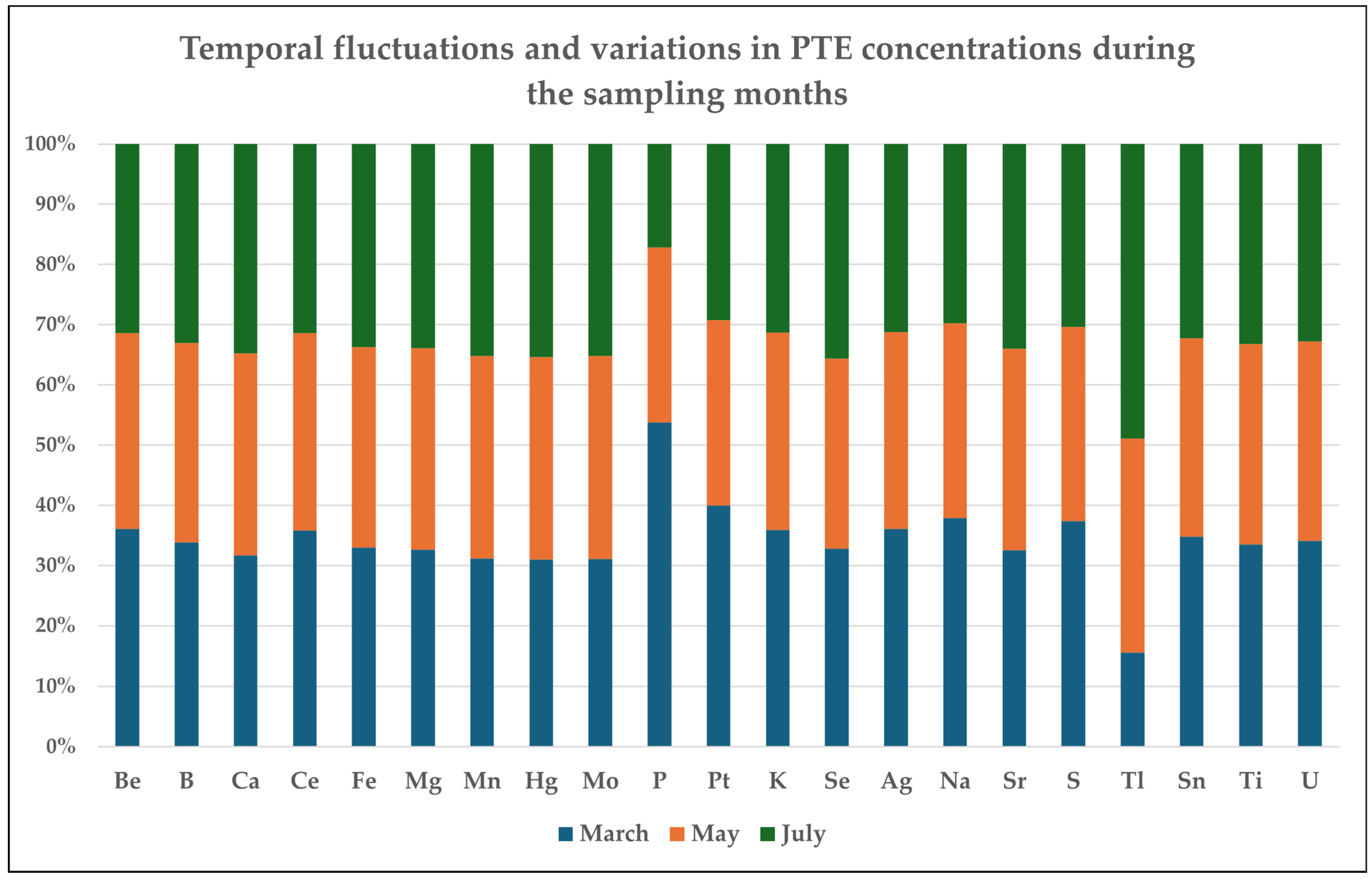
3.2. Temporal Trends and Winter-to-Summer Patterns

The foundational spatiotemporal patterns for 12 key heavy metals (HMs) within this Thessaloniki biomonitoring campaign, including their basic ANOVA-derived significance regarding sampling month and location, were initially presented in Sfetsas et al. [21]. That study established the general responsiveness of Syntrichia moss to urban pollution gradients. Building upon this, the current investigation expands the elemental scope to twenty-one PTEs, incorporating nine additional elements not previously reported. While reaffirming the established ANOVA outcomes for common elements (

Table 5. Effects of temporal and spatial variation on PTE levels in Syntrichia moss.

Elements	Factors	df	Mean Squares	F-Statistics	p-Value	Model Adjusted R2
Be	Months	2	0.007286	5.07	0.013 **	79.23%
	Locations	15	0.017836	12.41	0.000 ***
B	Months	2	3.408	0.26	0.771 ns	74.78%
	Locations	15	135.181	10.39	0.000 ***
Ca	Months	2	77342816	2.42	0.106 ns	90.57%
	Locations	15	986819357	30.91	0.000 ***
Ce	Months	2	22.424	2.90	0.070 ns	74.88%
	Locations	15	77.913	10.08	0.000 ***
Fe	Months	2	304266	0.04	0.958 ns	74.05%
	Locations	15	70816331	10.07	0.000 ***
Mg	Months	2	132977	0.67	0.520 ns	94.66%
	Locations	15	11260505	56.56	0.000 ***
Mn	Months	2	29611	0.05	0.954 ns	52.42%
	Locations	15	2867061	4.58	0.000 ***
Hg	Months	2	0.001077	0.89	0.420 ns	77.62%
	Locations	15	0.014339	11.88	0.000 ***
Mo	Months	2	0.3143	1.44	0.253 ns	86.22%
	Locations	15	4.4830	20.55	0.000 ***
P	Months	2	4275261	104.83	0.000 ***	87.11%
	Locations	15	339493	8.32	0.000 ***
Pt	Months	2	0.000013	2.35	0.113 ns	82.61%
	Locations	15	0.000090	15.70	0.000 ***
K	Months	2	1268404	11.55	0.000 ***	70.87%
	Locations	15	792401	7.22	0.000 ***
Se	Months	2	0.014685	2.19	0.130 ns	78.38%
	Locations	15	0.081953	12.20	0.000 ***
Ag	Months	2	0.004897	0.56	0.578 ns	89.89%
	Locations	15	0.253965	28.93	0.000 ***
Na	Months	2	12586	3.39	0.047 **	68.68%
	Locations	15	28048	7.55	0.000 ***
Sr	Months	2	32.91	0.75	0.480 ns	82.70%
	Locations	15	700.34	16.01	0.000 ***
S	Months	2	336447	7.39	0.002 ***	80.47%
	Locations	15	594374	13.06	0.000 ***
Tl	Months	2	0.233731	119.11	0.000 ***	84.65%
	Locations	15	0.004960	2.53	0.015 **
Sn	Months	2	0.4811	0.31	0.732 ns	88.95%
	Locations	15	40.1792	26.30	0.000 ***
Ti	Months	2	36.5	0.02	0.981 ns	75.00%
	Locations	15	19604.9	10.53	0.000 ***
U	Months	2	0.006034	0.19	0.831 ns	89.43%
	Locations	15	0.895999	27.63	0.000 ***

R = correlation coefficient, ns = non-significant differences; ** = p-value < 0.05; *** = p-value < 0.001 (very strong significance). ANOVA was performed to define the temporal and spatial effects in the PTE concentrations.

), our primary focus herein shifts to elucidating the unique temporal and spatial behaviors of these newly analyzed PTEs and, crucially, leveraging the complete 21-PTE dataset for a comprehensive source apportionment through integrated multi-index analysis and PMF modeling.

Two-way ANOVA results (Table 5) highlighted significant month effects for select elements with high R² values (68.7–94.7). P exhibited the most significant decrease, dropping by 60% from March to July (R² = 87.1%), in agreement with previous study [45], and similarly, K by 30% (R² = 70.9%). S decreased significantly (R² = 80.5%), likely reflecting reduced winter heating emissions [46,47]. Be decreased slightly (R² = 79.2%), with March to July differences linked to combustion of solid fuels. Na showed a modest decline (R² = 68.7%), tied to reduced sea-salt deposition. In contrast, Tl surged 3.5-fold from March to July (R² = 84.7%), indicating strong anthropogenic inputs. This aligns with heightened summer activities, such as tourism-driven traffic [41] and industrial operations [48]. Elements like P, K, and S exhibited a pronounced decrease from March to July, likely reflecting reduced heating emissions (Figure 2). Conversely, Tl showed a substantial increase over the same period, potentially linked to heightened summer traffic and tourism. Other elements, such as Fe and Pt, displayed relatively stable proportions across the months, suggesting more consistent sources. These fluctuations highlight the influence of seasonal anthropogenic activities and meteorological factors on PTE deposition patterns. The stark rise in Tl necessitates monitoring of summer emissions, while P/K trends could highlight moss physiology. Spatial stability in elements like Fe and Pt emphasizes localized contamination, requiring targeted mitigation. These findings underscore the interplay of geogenic and anthropogenic sources shaping elemental dynamics in the ecosystem. Thus, the winter-to-summer transition reflects the following: (1) Biological activity—dominant in P/K declines potentially due to moss growth. (2) Anthropogenic pressure—critical for Tl surge and S winter peak. (3) Environmental factors—reduced sea spray (Na) and temperature-mediated deposition (Be).

3.3. Spatial Trends in Elemental Concentrations

The temporal trends of PTEs were statistically assessed using two-way ANOVA (results in Table 5). As outlined in Section 2.6, prior to performing ANOVA, the PTE concentration data were tested for normality (Shapiro–Wilk test) and homogeneity of variances (Levene’s test). For most elements, the assumptions for ANOVA were adequately met, occasionally after log-transformation of the data. Given the balanced design and sample size, ANOVA was considered a robust method for evaluating the main effects of ‘Sampling Month’ and ‘Location’.

The two-way ANOVA (Table 5) confirmed location as the dominant factor, with highly significant spatial effects for all elements and high R² values (52.4–94.7%), underscoring strong heterogeneous spatial dependence identifying distinct elemental profiles for the three sampling clusters:

The City Center exhibited the most pronounced enrichment of PTEs (

Table 6. Levels of potentially toxic elements (mg/kg) in Syntrichia moss samples from 16 urban Thessaloniki locations.

Location	Type	Be	B	Ca	Ce	Fe	Mg	Mn	Hg	Mo	P	Pt	K	Se	Ag	Na	Sr	S	Tl	Sn	Ti	U
L01	M	0.32	16.0	74,421.4	21.0	10,353.3	4496.7	265.2	0.05	1.05	320.9	0.003	2877.6	0.38	0.10	136.1	70.6	536.1	0.24	1.90	258.6	0.86
L02	M	0.09	30.2	19,985.7	4.6	2369.1	2240.4	109.9	0.07	0.86	750.6	0.002	3801.7	0.11	0.11	73.3	31.4	1295.2	0.25	0.88	82.5	0.15
L03	M	0.41	29.8	55,326.2	24.7	12,076.2	4888.2	311.5	0.06	0.96	392.8	0.005	3980.8	0.55	0.09	148.8	66.3	540.7	0.19	1.64	307.3	0.69
L04	C	0.23	33.2	49,967.5	14.6	9012.5	7869.0	238.4	0.06	3.24	708.5	0.004	3365.0	0.47	0.13	299.1	80.4	1616.2	0.20	4.40	259.2	2.36
L05	C	0.29	35.8	49,463.1	20.1	11,515.6	4412.5	276.0	0.12	4.44	1326.5	0.017	4207.6	0.48	0.36	188.2	73.2	1982.9	0.19	12.51	311.6	0.77
L06	C	0.40	35.5	36,317.7	20.3	12,163.9	4471.3	354.4	0.11	2.41	1628.9	0.004	3945.6	0.65	0.21	164.7	68.6	1886.6	0.23	10.73	279.4	0.69
L07	I	0.33	33.0	30,391.6	20.3	15,520.4	3536.9	556.2	0.09	1.95	1146.7	0.002	4250.0	0.65	0.27	162.9	44.6	1220.4	0.26	4.66	365.3	0.59
L08	I	0.26	46.2	48,610.4	16.7	19,565.1	3847.2	806.0	0.11	2.84	1009.9	0.003	4345.9	0.51	0.21	242.4	54.8	1500.5	0.19	6.28	321.2	1.03
L09	I	0.31	31.3	48,697.5	21.7	12,953.0	3889.8	427.4	0.06	1.65	1121.1	0.003	3965.5	0.63	0.10	221.8	61.1	1409.2	0.28	2.60	395.7	1.11
L10	R	0.33	39.5	56,382.0	19.2	12,310.2	3874.5	391.3	0.11	2.51	1205.5	0.005	5034.6	0.57	0.20	482.6	74.2	1763.3	0.19	3.05	378.0	1.79
L11	C	0.31	30.7	70,344.6	21.3	15,117.9	5317.7	383.5	0.21	4.35	939.1	0.021	4156.6	0.48	1.26	298.1	95.1	1753.7	0.30	8.33	328.0	1.25
L12	C	0.27	39.9	48,958.1	19.5	21,724.9	4391.4	3249.9	0.14	4.05	876.1	0.006	4323.8	0.45	0.31	211.9	74.5	1662.4	0.32	7.21	318.4	0.79
L13	I	0.34	32.9	71,358.0	17.6	16,223.7	4107.4	3080.3	0.26	2.14	799.2	0.005	3506.2	0.40	0.26	210.0	67.5	1139.7	0.28	4.55	326.2	0.88
L14	C	0.29	36.2	24,067.5	15.1	13,004.8	10,636.3	351.9	0.26	1.33	675.4	0.002	3502.2	0.84	0.03	226.9	48.1	990.3	0.22	0.66	226.8	1.31
L15	A	0.25	25.0	59,230.7	10.4	6595.7	4718.6	173.5	0.10	1.52	751.3	0.003	4121.5	0.29	0.05	349.4	65.5	1105.2	0.24	1.18	180.5	1.24
L16	A	0.19	30.0	14,300.5	11.7	6695.8	3903.2	183.0	0.17	0.97	1101.1	0.001	4569.2	0.45	0.06	189.3	53.9	915.0	0.26	0.88	202.5	0.24
Mean		0.29	32.8	47,363.9	17.4	12,325.1	4787.6	697.4	0.12	2.27	922.1	0.005	3997.1	0.49	0.24	225.3	64.4	1332.3	0.24	4.47	283.8	0.98
Median		0.30	33.0	49,210.6	19.4	12,237.0	4402.0	353.2	0.11	2.04	907.6	0.004	4051.1	0.48	0.17	211.0	66.9	1352.2	0.24	3.72	309.4	0.87
SE		0.02	1.62	4390.20	1.23	1176.07	468.97	236.64	0.02	0.30	81.43	0.00	124.40	0.04	0.07	23.41	3.70	107.74	0.01	0.89	19.57	0.13
RSD%		286.4	405.0	169.7	253.0	162.0	155.2	26.3	85.4	91.5	183.1	0.5	703.2	208.7	16.31	140.7	335.0	209.1	510.3	26.0	262.6	85.8
Reference Elemental Concentrations from Moss Grown in a Controlled Environment
BsV1		0.017	27.4	16,206.2	0.834	506.7	3437.8	33.0	0.07	0.281	1037.1	0.001	2995.2	0.21	0.03	115.5	59.6	1305.8	0.01	0.66	19.5	0.13
BsV2		0.022	29.6	14,671.6	1.119	569.7	3100.4	42.6	0.06	0.283	1161.2	0.001	3278.8	0.21	0.04	95.7	54.8	1762.8	0.01	0.46	19.6	0.16
BsV3		0.021	29.1	15,155.5	1.044	531.1	3590.0	38.2	0.05	0.258	924.8	0.001	3277.2	0.19	0.04	99.0	58.3	1167.2	0.01	0.40	17.9	0.15
Mean		0.020	28.7	15,344.4	1.00	535.8	3376.1	37.9	0.06	0.3	1041.0	0.001	3183.7	0.20	0.04	103.4	57.6	1411.9	0.01	0.50	19.0	0.15
SE		0.01	0.54	369.84	0.07	14.97	118.12	2.27	0.00	0.01	55.74	0.001	76.97	0.01	0.01	5.00	1.17	146.92	0.00	0.07	0.45	0.01
RSD%		3.3	1.4	1.2	4.31	0.89	1.8	0.7	1.11	2.5	0.4	3.333	2.9	2.27	10.26	4.4	1.3	8.1	2.05	10.84	2.6	0.45

BsV: baseline sample values; SE = standard error; RSD = relative standard deviation. (M = Motorway, A = Airport Surroundings, C = City Center, I = Industrial Zone, R = Road Adjacent to Oil and Fuel Terminal).

), with Fe (21,724.9 mg/kg at L12, 1.76 × mean) and Mn (3249.9 mg/kg at L12, 4.65 × mean) being exceptionally elevated, aligning with the combustion of fossil fuels [49,50]. Sn (12.51 mg/kg at L05, 2.8 × mean) is used on steel to prevent corrosion, in alloys in the manufacture of brakes, organotin compounds, etc. [51]. Ag (1.26 mg/kg at L11, 5.25 × mean) is potentially tied to combustion of wastes, electronics, catalysts, and batteries [52,53]. Mo (4.44 mg/kg at L05, 1.96 × mean) elevations can originate from several urban sources [54] and Se (0.84 mg/kg at L14, 1.71 × mean) highlighted emissions from burning of fossil fuel [55]. Finally, Pt, a well-known tracer for catalytic converters and fuel cells, exhibited distinctly elevated concentrations at locations L11, L05, and L12 [56].

The Industrial Area showed dominance of Fe (16,223.7 mg/kg at L13, 1.32 × mean) potentially originating from steel manufacturing and coal combustion [57] and Ca (71,358.0 mg/kg at L13, 1.51 × mean), being linked to industrial emissions and the wind erosion of soils and subsequent dissolution of Ca bearing minerals [58]. U (1.79 mg/kg at L10, 1.83 × mean) is primarily associated with industrial processes, while its particles can be transported over long distances [59]. Notably, Na (482.6 mg/kg at L10, 2.14 × mean) and K (5034.6 mg/kg) align with sea-salt aerosol influence, given its proximity of Thessaloniki’s coastline [60].

The Motorway/Airport Area was dominated by Ca, Fe, Mn, Se (74,421.4 at L01, 21,724.9 at L12, 4496.7 at L01 and 0.55 mg/kg at L03, respectively), and Sn (107.3 mg/kg at L06, 24.0 × mean). These elemental signatures reflect the influence of vehicular emissions (brake and tire wear, abrasion, resuspension, etc.) as reported in previous studies [61,62]. In contrast, L02 (motorway) demonstrated consistently low PTE concentrations, forming a distinct outlier. This status demonstrates how micro-environmental factors can alter deposition patterns, such as localized wind outlines, vegetation barriers, or topography, that mitigate pollutant deposition [63].

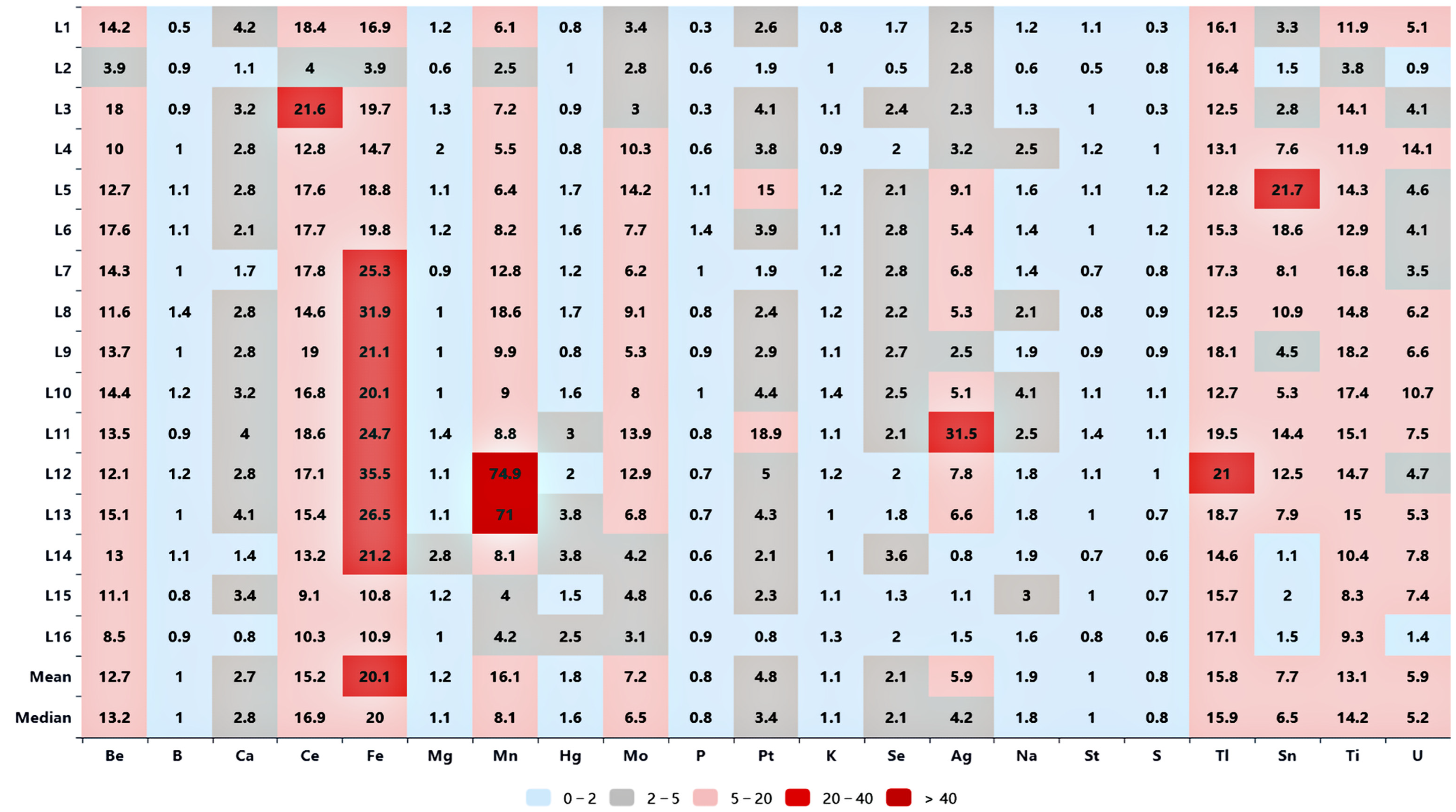
3.4. Multi-Index Approach Synergizing CF, EF, PLI, and PMF

The integration of CF, EF, PLI, and PMF analyses provides a robust framework for identifying spatial contamination clusters and evaluating pollution sources, though their combined application reveals critical interdependencies and methodological corrections (Figure 3, Figure 4, Figure 5 and Figure 6). PMF identified three primary sources contributing to PTE deposition in Thessaloniki: Factor 1 (17%) (F1) reflects crustal sources, Factor 2 (35%) (F2) represents industrial emissions, and Factor 3 (48%) (F3) captures traffic-related emissions (Figure 3). While PMF’s F1 groups Ti with crustal elements (Ca, Mg, Na), CF (Figure 4a,b and Figure 5) and EF (Figure 6), calibrated to laboratory-derived backgrounds (Ti:19 mg/kg), reveal severe anthropogenic enrichment (CF = 14.9; EF = 13.1), suggesting PMF’s crustal attribution may mix geogenic and anthropogenic dust resuspension. This contradiction underscores CF/EF’s role in grounding PMF’s statistical outputs in empirical baselines, ensuring anthropogenic signals are not diluted. Similarly, PMF clarifies ambiguities left by standalone indices, while CF/EF identify “extreme” industrial/traffic contamination (Sn: CF 24.8, EF 21.7; Ag: CF = 36.0, EF = 31.5) and PLI (Figure 7) aggregates city-wide risk (PLI = 3.8), PMF disentangles mixed sources (Pt in F2 and 3) and isolates micro-environmental outliers like L02 (PLI = 1.8), where vegetation mitigates deposition.

However, PMF’s low R² for Ag and Tl reveals gaps in resolving rare/diffuse emissions, where CF/EF’s element-specific focus fills critical gaps, Ag CF/EF peaks at L11, implicating port-related emissions, a source that PMF only partially captures. Conversely, PLI’s holistic risk assessment, though lacking granularity, underrepresenting Sn localized hazard in Motorway/Airport, complements PMF’s source mapping and CF/EF’s severity metrics. The hybrid approach thus prioritizes as follows: City Center—Sn/Ag/Pt controls (CF/EF > 20; PMF F2/F3), overriding PMF’s partial resolution of Ag origin; Industrial Area—Fe/Mn/U reductions (CF > 40; PMF F2), aligning steel/coal emissions with CF/EF’s severity; Motorway/Airport—Sn/Be mitigation (CF/EF > 18; PMF F3), addressing PLI’s underestimation of road dust risks. The combined analysis shows that while no single index is universally superior, their synergy corrects overestimations, e.g., Ti’s PMF misclassification, and resolves mixed sources, proving essential in urban ecosystems. CF/EF anchor interpretations in measurable contamination thresholds, PMF disentangles source complexity, and PLI contextualizes macro-impacts, collectively bridging statistical patterns with actionable environmental insights. This multi-index approach not only refines source apportionment but also highlights the necessity of integrating empirical baselines with statistical models to ensure accurate and actionable pollution mitigation strategies.

The PMF analysis yielded a robust solution with a total Q(true) value of 7356.4 and Q(robust) value of 7128.2, indicating a good fit of the model. The difference between Q(true) and Q(robust) suggests that extreme values had minimal impact on the factorization process, reinforcing the model’s stability. The determination of the optimal number of factors was based on a combination of Q-value minimization, interpretability of source profiles, and the diminishing returns in variance explained beyond three factors. A three-factor solution was selected, capturing 48% of total variance in traffic-related emissions, 35% in industrial emissions, and 17% in crustal contributions. While PMF effectively resolved major pollution sources, some uncertainties remain, particularly in attributing diffuse emissions such as port activities and mixed combustion sources. The presence of low R² values for certain elements (e.g., Ag and Tl) suggests potential underestimation of rare emission events or over-representation of background sources. These limitations highlight the importance of integrating PMF with contamination indices and empirical baselines to refine source apportionment accuracy. Despite these uncertainties, the model’s overall performance confirms the utility of PMF for distinguishing urban air pollution contributors and guiding mitigation strategies.

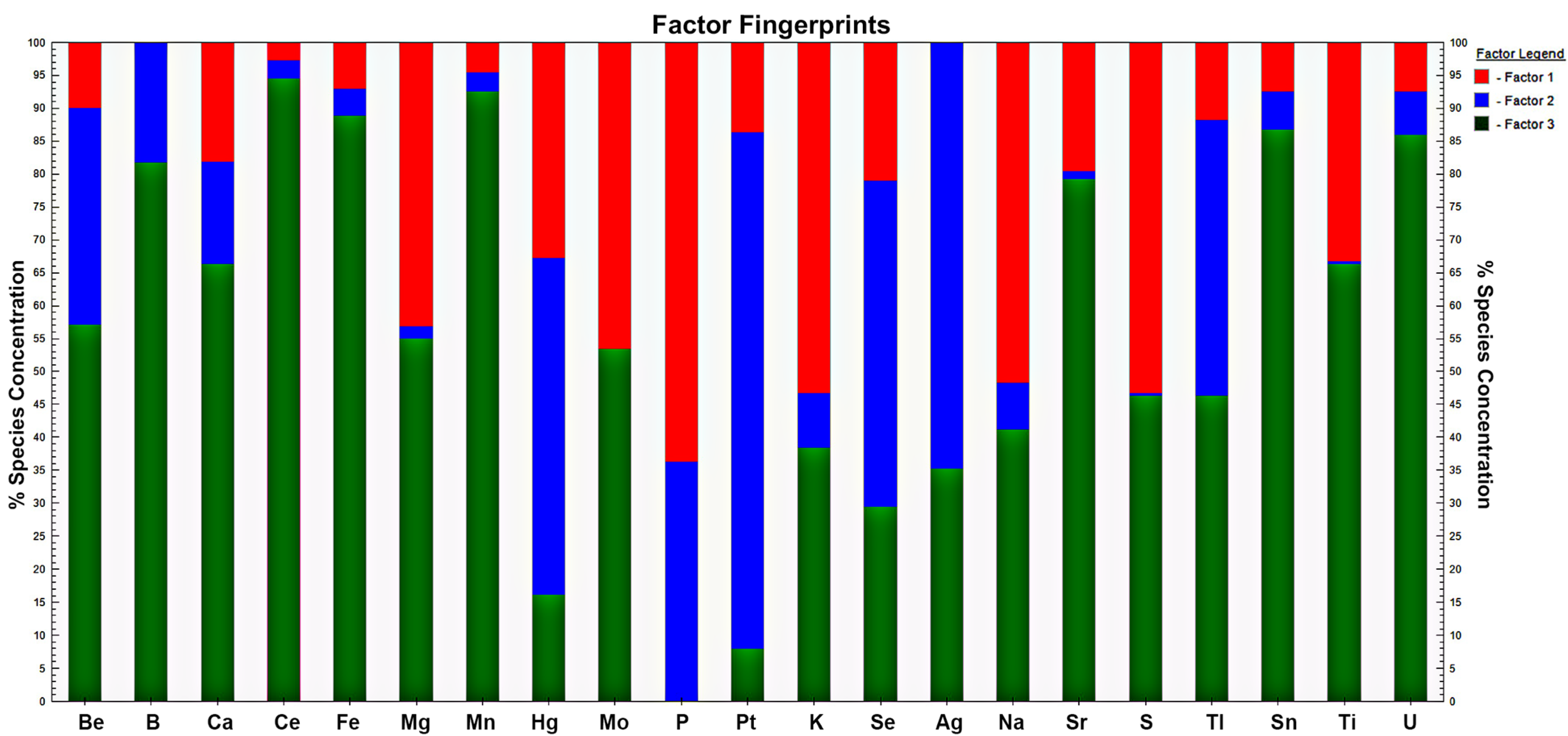
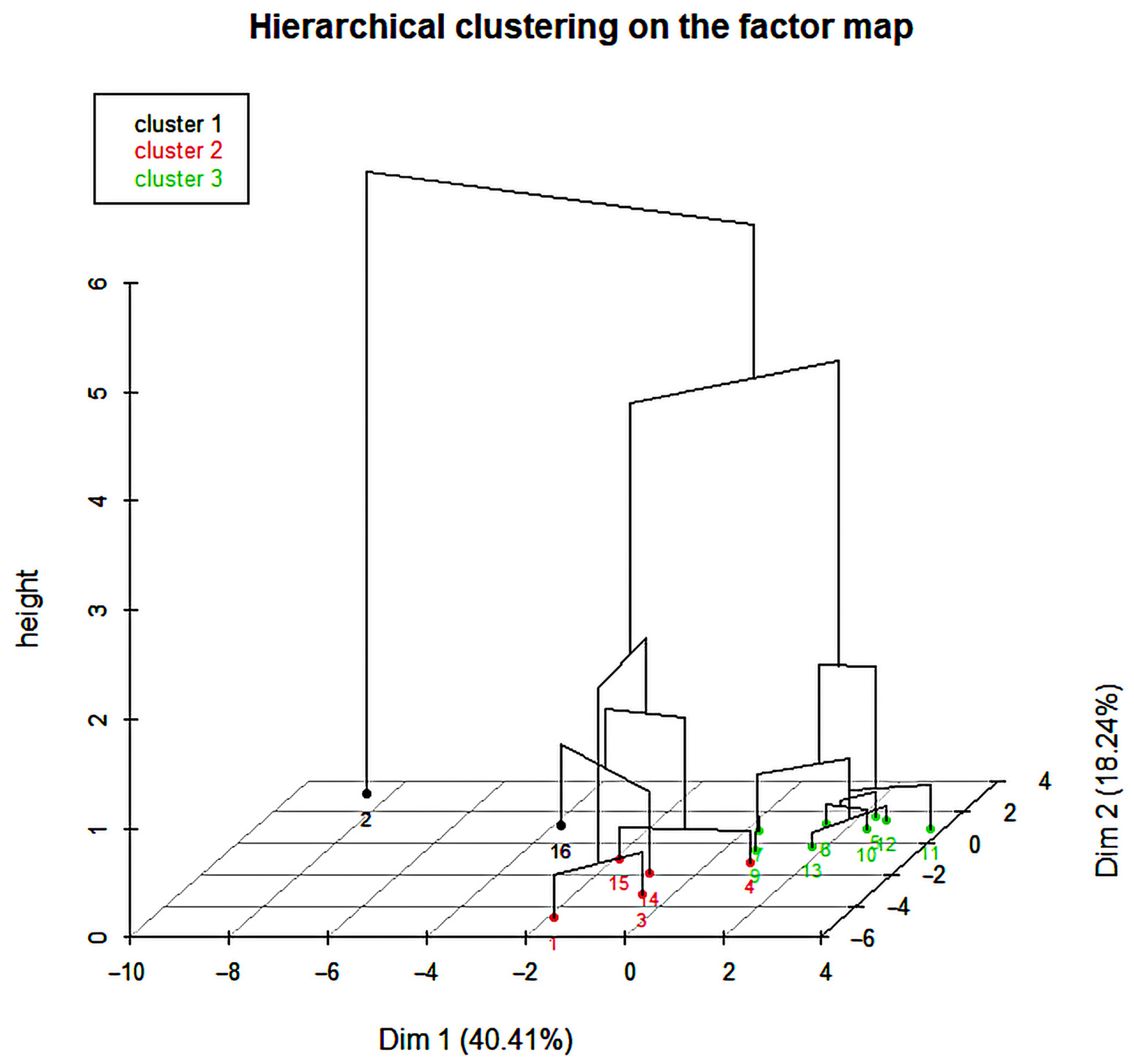
3.5. Multivariate Analysis of PTE Contamination Patterns

Multivariate analyses elucidated contamination dynamics, refining spatial clusters while reconciling discrepancies between geochemical indices and source apportionment. PCA (Figure 7 and Figure 8) resolved two dominant sources: PC1 (53.1% variance) grouped Fe, Ti, Ce, Be, U, and Sn, strongly associating with industrial emissions, particularly at L07–L13; Elevated Mn at L12/L13, aligning with PMF’s industrial factor and spatial clusters. However, Ti’s inclusion in PC1 conflicted with PMF’s crustal attribution, where CF/EF metrics (CF = 14.9; EF = 13.1) confirmed “severe” anthropogenic enrichment, suggesting PCA mixed natural dust resuspension (constructions) with industrial emissions. PC2 (18.9% variance) linked Mg, Ca, K, and S to crustal/construction activities, consistent with PMF’s F1 but contrasting with spatial analyses that tied these elements to traffic-linked resuspension in the City Center. HCPC (Figure 8) further refined the spatial patterns by grouping the sampling locations based on their overall PTE profiles. Figure 8 visualizes this clustering, displaying a dendrogram where branch heights indicate dissimilarity, and distinct colored groups represent the identified clusters based on their principal component scores. A combined analysis of PCA and HCPC results identified three distinct clusters described below.

Cluster 1 (Red) (L01, L03, L04, L05, L15, L16) exhibited mixed traffic-industrial influences, with L01/L03 reflecting motorway emissions (Tl, Ce) and L15/L16 airport abrasion, mirroring Motorway/Airport Area. L05′s transitional role (high Sn/Mo) bridged PMF’s hybrid traffic-industrial sources, though its dual classification (City Center vs. transitional) underscored methodological divergences between spatial zoning and statistical linkages.

Cluster 2 (Green) (L06–L13, L05) confirmed industrial dominance, with L12/L13′s Mn/Fe peaks and L11′s Ag hotspot (CF = 36.0), reinforcing PMF’s industrial factor.

Cluster 3 (Black) (L02) remained a low PTE outlier due to physical barriers, validated across all analyses. While PCA and PMF resolved broad source categories, CF/EF’s element-specific severity metrics exposed limitations in statistical models, particularly for Ti dual attribution and Ag diffuse emissions. Integrating multivariate methods with PMF and contamination indices highlighted the necessity of empirical baselines to separate overlapping sources (crustal vs. anthropogenic dust), ensuring robust interpretations for targeted mitigation. These findings underscore the complementary role of multivariate techniques in refining spatial clusters while emphasizing the need for localized soil validation to resolve uncertainties in source distribution, particularly for elements like Ti, where geogenic and anthropogenic contributions remain intertwined.

3.6. Understanding the PTE Contamination Sources in Thessaloniki

The results of this study show that Thessaloniki’s PTE contamination is driven by three interconnected sources, crustal, industrial, and traffic-related (17:35:48%) with spatial and seasonal dynamics further modulated by anthropogenic and environmental factors. Industrial zones, particularly L12 and L13, exhibit pronounced F2 dominance, characterized by Fe (F2:65%) and Mn (F2:68%) enrichment linked to steel manufacturing and coal combustion [64], confirmed by CF values > 40 and mirroring contamination patterns in Belgrade’s industrial corridors [65]. Concurrently, Ag F2 association (66%) at L11, adjacent to the port, reflects waste incineration and electronic waste disposal [52], though CF/EF metrics (CF = 36.0) exposed PMF’s underestimation of this localized anthropogenic signal. Traffic emissions (F3:48%) dominate motorway–airport clusters (L01, L03, L15, L16), with Tl (F3:48%), Ce (F3:54%), and Ti (F3:71%) tied to non-exhaust vehicular abrasion [66], while Sn dual allocation (F2/F3, 69/26%) underscores secondary industrial inputs [51]. The City Center’s mixed profile blends F3-driven resuspension (Mg: 72%, S: 84%) from construction and traffic [47] with harbor-influenced Ag/Mo (F2: 66%, F3: 81%), paralleling Mediterranean port studies [67]. Seasonal PMF variations clarify temporal shifts: winter S/K peaks (F3:71/84%) align with residential biomass burning and sulfur-rich fuel use [68,69], while summer Tl elevations (F3:48%) correlate with tourism-driven traffic, a pattern aggravated by Thessaloniki’s coastal urban layout [48]. It is important that the CF/EF integration resolved the PMF uncertainties: Ti conflicting F1/F3 attribution (9/71%) versus CF = 14.9 confirmed anthropogenic dust (construction and traffic), while PLI = 3.8 prioritized City Center Sn/Ag/Pt hotspots (CF/EF > 20) despite PMF’s diffuse sourcing. The anthropogenic dust component contributing to Tl, particularly when linked to construction activities (F3-driven resuspension), may also reflect contributions from cement-related activities, such as cement production and related raw materials (like clinker) are indeed handled during transportation (e.g., port activities). Tl can be present as a trace impurity in raw materials for cement production and emitted during kiln operations or found in the final cement product [70,71]. Given the presence of cement facilities and the handling of cementitious materials at the port, fugitive dust from these sources or the resuspension of historically contaminated soil could contribute to the observed Tl signatures, particularly in areas with significant construction or soil disturbance. Moreover, the outlier status of L02 (PLI = 1.8), with its vegetation-mediated deposition reduction, highlights micro-scale mitigation potential absent in PMF’s macro-scale factors. Thus, these findings necessitate targeted strategies: stricter F2 controls on industrial Fe/Mn emissions, F3-focused adoption of low-abrasion vehicular materials to curb Tl/Sn, and enhanced port waste management to address Ag/Mo [53,72].

Beyond local and regional anthropogenic activities, the influence of long-range transported natural aerosols, particularly Saharan dust, warrants consideration as a contributor to atmospheric PTE levels in Thessaloniki, a common phenomenon in the Mediterranean [73]. In a long-term study (1984–2012), Saharan dust deposition in the Aegean Sea region near Attica was measured and varied between 61 and 199 μg/m²/day during dust events, with crustal enrichment being most pronounced in summer [74]. This gives an indication of the potential magnitude of such inputs, although specific fluxes for Thessaloniki would vary [75]. These dust events, most frequent in spring and summer, transport significant quantities of crustal material, enriching the atmosphere with elements such as Al, Si, Ca, Fe, and Ti. While our PMF model identified a ‘crustal material’ factor (F1), this likely represents a composite of locally resuspended soil and road dust, as well as these episodic inputs of Saharan dust [76]. Differentiating these within the F1 profile is challenging without specific event-based analysis or unique tracers. However, the occurrence of such dust events during or preceding our sampling campaigns could elevate the background concentrations of these geogenic elements in the Syntrichia moss, thereby influencing the interpretation of anthropogenic enrichment factors and the precise composition of the PMF crustal source profile. The presence of Saharan dust could have several implications for our findings outlined below.

• Baseline Levels: It could elevate the background concentrations of major crustal elements (Al, Fe, Ca, Mg, Ti, Si if measured) in the moss samples, particularly during or shortly after dust events. This is pertinent as our sampling campaign spanned March to July, a period when Saharan dust events can occur.
• EF Interpretation: Elevated natural background levels of these elements due to desert dust could influence the calculation and interpretation of EFs for other elements that might also have anthropogenic sources but are normalized to a crustal reference element (like Ti or Al). If the reference element’s concentration is inflated by desert dust, it could potentially mask or underestimate anthropogenic enrichment for other PTEs.
• Source Apportionment by PMF: While PMF identified a crustal factor, it may not be able to fully distinguish between local geogenic sources and long-range transported desert dust without specific chemical tracers or mineralogical markers (e.g., palygorskite), or characteristic elemental ratios like Ca/Fe as suggested by Vasilatou et al. [74] that are more uniquely associated with Saharan dust.

By synergizing PMF’s source apportionment with CF/EF’s empirical severity thresholds and PLI’s holistic risk aggregation, this multi-index framework bridges statistical rigor with actionable insights. These findings emphasize Thessaloniki’s contamination profile as a product of industrial intensity, traffic density, and maritime operations, necessitating integrated mitigation strategies that target sector-specific emissions—such as stricter industrial controls, low-abrasion vehicular materials, and enhanced port waste management—while addressing seasonal biomass burning. The interplay of spatial hotspots and temporal trends underscores the need for adaptive policies that reconcile persistent industrial sources with fluctuating anthropogenic activities, ensuring holistic air quality management in Thessaloniki’s complex urban ecosystem.

The PTE contamination patterns observed in Thessaloniki align broadly with findings from other complex urban-industrial environments. Belgrade is an example, where active moss biomonitoring identified industrial corridors as major pollution sources, particularly linked to elements like Fe and Mn [77]; our study confirms pronounced industrial hotspots dominated by these metals. Although Thessaloniki’s higher traffic contribution, 48% vs. Belgrade’s ~35%, reflects tourism-driven emissions, both cities show industrial Fe/Mn enrichment, but Thessaloniki uniquely highlights Tl spikes (3.5× summer increase). Salerno’s focus on S emissions mirrors Thessaloniki’s winter S decline. Traffic-related emissions, a ubiquitous urban issue also influencing soil contamination patterns in Salerno [43], are clearly resolved in Thessaloniki, notably through distinct tracers like Tl and Pt, yet Thessaloniki’s integration of PMF and multi-index analysis offers finer source resolution. Seasonal trends in Thessaloniki (e.g., summer Tl peaks) contrast with Belgrade’s less pronounced seasonality, underscoring Mediterranean cities’ vulnerability to tourism emissions. Methodological advancements in Thessaloniki, including high-resolution sampling (1.48 samples/km²) and CF validation, address limitations in Belgrade’s spatial resolution and Salerno’s reliance on soil analysis. These comparisons highlight region-specific drivers and the value of multi-technique approaches in urban air quality assessments.

3.7. Considerations and Limitations

The calculation of CF and EF relies on baseline elemental data from mosses cultivated in a controlled environment [21]. We acknowledge that utilizing such laboratory-derived baselines, while essential for standardization in the absence of verifiable local uncontaminated sites, represents a potential limitation. Field conditions could influence background elemental uptake differently than controlled settings. While lab-derived B baselines standardize comparisons, field conditions may introduce variability. Nevertheless, Boron’s low reactivity with pollutants [33] reduces this risk, reinforcing its safety as a reference. However, the robustness of our main conclusions regarding contamination sources and spatial patterns is strongly supported by several factors: (1) the extremely high CF and EF values observed for key anthropogenic pollutants (e.g., Sn, Ag, Tl, Fe) far exceed any plausible minor variations in baseline levels, indicating significant enrichment regardless of the exact reference point; and (2) the strong convergence of these index-based findings with independent source apportionment results from PMF modeling and multivariate statistical analysis provides cross-validation for the identified pollution hotspots and contributing sources.

While this study demonstrates the efficacy of Syntrichia moss biomonitoring for urban air quality assessment, certain limitations warrant future methodological refinements. Specifically, potential soil-derived contamination of elements like Ca, Mg, and Fe—despite rigorous field and laboratory protocols—highlights the need for advanced source discrimination tools. Isotopic tracing offers a promising avenue to disentangle geogenic vs. anthropogenic contributions. Furthermore, the study’s constrained temporal resolution from whole-season sampling necessitates continuous monitoring to capture finer meteorological variability and short-term events.

Additionally, controlled-environment baseline moss data may underestimate urban bioavailability, and city-specific emission profiles limit broader applicability, underscoring the need for multi-city, multi-species biomonitoring in future work. Despite these constraints, the study’s spatial-temporal patterns robustly identified industrial, vehicular, port, and residential heating as key PTE contributors in Thessaloniki.

4. The Effects of PTEs on Human Health

Elevated PTE levels primarily driven by anthropogenic activities, pose significant human health risks since they can lead to toxicity and adverse health outcomes, even though these elements are not listed as hazardous air pollutants [78]. Ce induces oxidative stress and lung inflammation [79]. Fe, Mn, and Ti elevate chronic obstructive pulmonary disease, neurodevelopmental impairment, and pulmonary inflammation, respectively [80,81]. Tl, which is one of the most toxic and destructive heavy metals for human and environmental health, has a higher level of chronic and acute toxicity in comparison to many harmful elements, such as Pb, Hg, Cd, while As exhibits neurotoxic potency [48,82]. Pt nanoparticles trigger anemia, nephrotoxicity, and DNA damage [83]. Thus, health risks vary by level, source proximity, and exposure duration, amplifying vulnerabilities and necessitating targeted biomonitoring to assess public health impacts.

5. Conclusions

This study successfully demonstrates that integrating Syntrichia moss biomonitoring with a suite of data analysis tools (CF, EF, PLI, PMF) provides a powerful and nuanced approach for assessing air quality and apportioning pollution sources within complex urban landscapes like Thessaloniki. The approach revealed significant anthropogenic contamination, with industrial zones (Fe, Mn, Sn) and traffic corridors (Tl, Ce, Pt) emerging as persistent hotspots. Contamination indices provided essential severity benchmarks and reinforced the PMF outputs, which identified three dominant pollution sources: crustal/geogenic (17%), industrial (35%), and traffic-related emissions (48%). Crucially, the synergy between the contamination indices providing empirical severity benchmarks and PMF offering refined source apportionment proved essential for validating hotspots and resolving ambiguities that might arise from using either approach in isolation. Seasonal trends—such as the increase in Tl and the decrease in heating-associated elements (P, K, S)—reflected the influence of changing human activities and meteorological conditions.

This multi-index-PMF framework applied to Syntrichia moss offers a high-resolution, sustainable, and cost-effective alternative to traditional monitoring networks, especially in areas with limited sensor coverage. By disentangling anthropogenic from geogenic contributions and resolving emission-sector signatures, the method informs targeted, EU-aligned air quality strategies to safeguard urban health. Its affordability, adaptability, and spatial granularity make it an especially attractive option for municipalities seeking data-driven environmental governance.

Limitations include potential soil influence on element levels (particularly Ca, Fe, Mg), which could be addressed in future studies through isotopic tracing or local soil validation. Additionally, although the study captured seasonal variability, continuous and longer-term monitoring is needed to assess short-term fluctuations and infrastructure impacts, such as those from Thessaloniki’s new metro system.

Overall, this work provides a methodological blueprint and robust baseline for integrated biomonitoring approaches in urban air quality management, with relevance for cities across the Mediterranean and similarly challenged environments. By bridging scientific evidence with actionable environmental policy, this framework empowers decision-makers to prioritize interventions that reduce exposure to hazardous pollutants and protect public health, particularly among vulnerable urban populations.

References

1. Power, A.L.; Tennant, R.K.; Stewart, A.G.; Gosden, C.; Worsley, A.T.; Jones, R.; Love, J. The evolution of atmospheric particulate matter in an urban landscape since the Industrial Revolution. Sci. Rep. 2023, 13, 8964. [Google Scholar] [CrossRef] [PubMed]
2. James, N. Urbanization and Its Impact on Environmental Sustainability. J. Appl. Geogr. Stud. 2024, 3, 54–66. [Google Scholar] [CrossRef]
3. Mistri, M.; Munari, C.; Pagnoni, A.; Chenet, T.; Pasti, L.; Cavazzini, A. Accumulation of trace metals in crayfish tissues: Is Procambarus clarkii a vector of pollutants in Po Delta inland waters? Eur. Zool. J. 2020, 87, 46–57. [Google Scholar] [CrossRef]
4. Streit, B. Bioaccumulation processes in ecosystems. Experientia 1992, 48, 955–970. [Google Scholar] [CrossRef]
5. Lu, Y.; Wang, R.; Zhang, Y.; Su, H.; Wang, P.; Jenkins, A.; Ferrier, R.C.; Bailey, M.; Squire, G. Ecosystem health towards sustainability. Ecosyst. Health Sustain. 2015, 1, 11878976. [Google Scholar] [CrossRef]
6. Rüegg, S.R.; Häsler, B.; Zinsstag, J. (Eds.) Integrated Approaches to Health: A Handbook for the Evaluation of One Health; Brill|Wageningen Academic: Wageningen, The Netherlands, 2018; ISBN 978-90-8686-324-2. [Google Scholar] [CrossRef]
7. Nieder, R.; Benbi, D.K.; Reichl, F.X. Macro- and Secondary Elements and Their Role in Human Health. In Soil Components and Human Health; Springer: Dordrecht, The Netherlands, 2018; pp. 257–315. ISBN 978-94-024-1221-5. [Google Scholar] [CrossRef]
8. Paseka, R.E.; Bratt, A.R.; MacNeill, K.L.; Burian, A.; See, C.R. Elemental Ratios Link Environmental Change and Human Health. Front. Ecol. Evol. 2019, 7, 378. [Google Scholar] [CrossRef]
9. Baishaw, S.; Edwards, J.; Daughtry, B.; Ross, K. Mercury in seafood: Mechanisms of accumulation and consequences for consumer health. Rev. Environ. Health 2007, 22, 91–114. [Google Scholar] [CrossRef]
10. Buch, A.C.; Brown, G.G.; Correia, M.E.F.; Lourençato, L.F.; Silva-Filho, E.V. Ecotoxicology of mercury in tropical forest soils: Impact on earthworms. Sci. Total Environ. 2017, 589, 222–231. [Google Scholar] [CrossRef] [PubMed]
11. Zhang, X.; Ekwealor, J.T.B.; Mishler, B.D.; Silva, A.T.; Yu, L.; Jones, A.K.; Nelson, A.D.L.; Oliver, M.J. Syntrichia ruralis: Emerging model moss genome reveals a conserved and previously unknown regulator of desiccation in flowering plants. New Phytol. 2024, 243, 981–996. [Google Scholar] [CrossRef]
12. Yang, R.; Li, X.; Yang, Q.; Zhao, M.; Bai, W.; Liang, Y.; Liu, X.; Gao, B.; Zhang, D. Transcriptional profiling analysis providing insights into desiccation tolerance mechanisms of the desert moss Syntrichia caninervis. Front. Plant Sci. 2023, 14, 1127541. [Google Scholar] [CrossRef]
13. Commission Decides to Refer GREECE to the Court of Justice. Available online: https://ec.europa.eu/commission/presscorner/detail/en/ip_20_2151 (accessed on 28 December 2024).
14. Natali, M.; Zanella, A.; Rankovic, A.; Banas, D.; Cantaluppi, C.; Abbadie, L.; Lata, J.-C. Assessment of trace metal air pollution in Paris using slurry-TXRF analysis on cemetery mosses. Environ. Sci. Pollut. Res. 2016, 23, 23496–23510. [Google Scholar] [CrossRef]
15. Donovan, G.H.; Jovan, S.E.; Gatziolis, D.; Burstyn, I.; Michael, Y.L.; Amacher, M.C.; Monleon, V.J. Using an epiphytic moss to identify previously unknown sources of atmospheric cadmium pollution. Sci. Total Environ. 2016, 559, 84–93. [Google Scholar] [CrossRef]
16. Steinnes, E.; Uggerud, H.T.; Pfaffhuber, K.A.; Berg, T. Atmospheric Deposition of Heavy Metals in Norway. National Moss Survey 2015; NILU: Kjeller, Norway, 2017; ISBN 978-82-425-2859-9. [Google Scholar]
17. Betsou, C.; Diapouli, E.; Tsakiri, E.; Papadopoulou, L.; Frontasyeva, M.; Eleftheriadis, K.; Ioannidou, A. First-Time Source Apportionment Analysis of Deposited Particulate Matter from a Moss Biomonitoring Study in Northern Greece. Atmosphere 2021, 12, 208. [Google Scholar] [CrossRef]
18. Lazo, P.; Kika, A.; Qarri, F.; Bekteshi, L.; Allajbeu, S.; Stafilov, T. Air Quality Assessment by Moss Biomonitoring and Trace Metals Atmospheric Deposition. Aerosol Air Qual. Res. 2022, 22, 220008. [Google Scholar] [CrossRef]
19. Chaligava, O.; Zinicovscaia, I.; Peshkova, A.; Yushin, N.; Frontasyeva, M.; Vergel, K.; Nurkassimova, M.; Cepoi, L. Major and Trace Airborne Elements and Ecological Risk Assessment: Georgia Moss Survey 2019–2023. Plants 2024, 13, 3298. [Google Scholar] [CrossRef]
20. Rajandu, E.; Kaljuvee, K.-L.; Kulp, M.; Kaasik, M.; Elvisto, T.; Küttim, M. Syntrichia ruralis as a suitable bioindicator for urban areas—The case study of Tallinn city. Folia Cryptogam. Est. 2024, 61, 25–34. [Google Scholar] [CrossRef]
21. Sfetsas, T.; Ghoghoberidze, S.; Karnoutsos, P.; Tziakas, V.; Karagiovanidis, M.; Katsantonis, D. Spatial and Temporal Patterns of Trace Element Deposition in Urban Thessaloniki: A Syntrichia Moss Biomonitoring Study. Atmosphere 2024, 15, 1378. [Google Scholar] [CrossRef]
22. Habibie, M.I.; Dayuf Yusuf, M.; Setyaningrum, N.; Pianto, T.A.; Nurdiansyah, N.; Aziz, M.L. Mapping and Monitoring Urban Areas Using Sentinel 1 and Sentinel 2. In Proceedings of the 2021 IEEE Asia-Pacific Conference on Geoscience, Electronics and Remote Sensing Technology (AGERS), Jakarta, Indonesia, 29–30 September 2021; pp. 125–129. [Google Scholar] [CrossRef]
23. Urošević, M.A.; Vuković, G.; Jovanović, P.; Vujičić, M.; Sabovljević, A.; Sabovljević, M.; Tomašević, M. Urban background of air pollution: Evaluation through moss bag biomonitoring of trace elements in Botanical garden. Urban For. Urban Green. 2017, 25, 1–10. [Google Scholar] [CrossRef]
24. Salo, H.; Paturi, P.; Mäkinen, J. Moss bag (Sphagnum papillosum) magnetic and elemental properties for characterising seasonal and spatial variation in urban pollution. Int. J. Environ. Sci. Technol. 2016, 13, 1515–1524. [Google Scholar] [CrossRef]
25. Nickel, S.; Schröder, W. Correlating elements content in mosses collected in 2015 across Germany with spatially associated characteristics of sampling sites and their surroundings. Environ. Sci. Eur. 2019, 31, 80. [Google Scholar] [CrossRef]
26. Lazo, P.; Stafilov, T.; Qarri, F.; Allajbeu, S.; Bekteshi, L.; Frontasyeva, M.; Harmens, H. Spatial distribution and temporal trend of airborne trace metal deposition in Albania studied by moss biomonitoring. Ecol. Indic. 2019, 101, 1007–1017. [Google Scholar] [CrossRef]
27. Hristozova, G.; Marinova, S.; Svozilík, V.; Nekhoroshkov, P.; Frontasyeva, M.V. Biomonitoring of elemental atmospheric deposition: Spatial distributions in the 2015/2016 moss survey in Bulgaria. J. Radioanal. Nucl. Chem. 2020, 323, 839–849. [Google Scholar] [CrossRef]
28. Svozilíková Krakovská, A.; Svozilík, V.; Zinicovscaia, I.; Vergel, K.; Jančík, P. Analysis of Spatial Data from Moss Biomonitoring in Czech–Polish Border. Atmosphere 2020, 11, 1237. [Google Scholar] [CrossRef]
29. Chaligava, O.; Shetekauri, S.; Badawy, W.M.; Frontasyeva, M.V.; Zinicovscaia, I.; Shetekauri, T.; Kvlividze, A.; Vergel, K.; Yushin, N. Characterization of Trace Elements in Atmospheric Deposition Studied by Moss Biomonitoring in Georgia. Arch. Environ. Contam. Toxicol. 2021, 80, 350–367. [Google Scholar] [CrossRef]
30. Šajn, R.; Bačeva Andonovska, K.; Stafilov, T.; Barandovski, L. Moss as a Biomonitor to Identify Atmospheric Deposition of Minor and Trace Elements in Macedonia. Atmosphere 2024, 15, 297. [Google Scholar] [CrossRef]
31. Fernández, J.A.; Aboal, J.R.; Carballeira, A. Identification of pollution sources by means of moss bags. Ecotoxicol. Environ. Saf. 2004, 59, 76–83. [Google Scholar] [CrossRef]
32. Sutherland, R.A. Bed sediment-associated trace metals in an urban stream, Oahu, Hawaii. Environ. Geol. 2000, 39, 611–627. [Google Scholar] [CrossRef]
33. Ejembi, J.I.; Nwigboji, I.H.; Franklin, L.; Malozovsky, Y.; Zhao, G.L.; Bagayoko, D. Ab-initio calculations of electronic, transport, and structural properties of boron phosphide. J. Appl. Phys. 2014, 116, 103711. [Google Scholar] [CrossRef]
34. Feng, B.; Zhang, J.; Zhong, Q.; Li, W.; Li, S.; Li, H.; Cheng, P.; Meng, S.; Chen, L.; Wu, K. Experimental realization of two-dimensional boron sheets. Nat. Chem. 2016, 8, 563–568. [Google Scholar] [CrossRef]
35. Tomlinson, D.L.; Wilson, J.G.; Harris, C.R.; Jeffrey, D.W. Problems in the assessment of heavy-metal levels in estuaries and the formation of a pollution index. Helgol. Meeresunters 1980, 33, 566–575. [Google Scholar] [CrossRef]
36. Norris, G.; Duvall, R.; Brown, S.; Bai, S. Positive Matrix Factorization (PMF) 5.0 Fundamentals and User Guide; United States Environmental Protection Agency: Washington, DC, USA, 2014. [Google Scholar]
37. De Beuckelaer, A. A closer examination on some parametric alternatives to the ANOVA F-test. Stat. Pap. 1996, 37, 291–305. [Google Scholar] [CrossRef]
38. Delacre, M.; Leys, C.; Mora, Y.L.; Lakens, D. Taking Parametric Assumptions Seriously: Arguments for the Use of Welch’s F-test instead of the Classical F-test in One-Way ANOVA. Int. Rev. Soc. Psychol. 2019, 32, 13. [Google Scholar] [CrossRef]
39. Wang, Y.; Dicle, C.; Sznaier, M.; Camps, O. Self Scaled Regularized Robust Regression. In Proceedings of the 2015 IEEE Conference on Computer Vision and Pattern Recognition (CVPR), Boston, MA, USA, 7–12 June 2015; IEEE: Piscataway, NJ, USA, 2015; pp. 3261–3269. [Google Scholar] [CrossRef]
40. Forero, P.A.; Giannakis, G.B. Sparsity-Exploiting Robust Multidimensional Scaling. IEEE Trans. Signal Process. 2012, 60, 4118–4134. [Google Scholar] [CrossRef]
41. Zhou, Z.-H.; Mao, J.-W.; Zhao, J.-Q.; Gao, X.; Weyer, S.; Horn, I.; Holtz, F.; Sossi, P.A.; Wang, D.-C. Tin isotopes as geochemical tracers of ore-forming processes with Sn mineralization. Am. Mineral. 2022, 107, 2111–2127. [Google Scholar] [CrossRef]
42. Merget, R.; Rosner, G. Evaluation of the health risk of platinum group metals emitted from automotive catalytic converters. Sci. Total Environ. 2001, 270, 165–173. [Google Scholar] [CrossRef] [PubMed]
43. Cicchella, D.; Zuzolo, D.; Albanese, S.; Fedele, L.; Di Tota, I.; Guagliardi, I.; Thiombane, M.; De Vivo, B.; Lima, A. Urban soil contamination in Salerno (Italy): Concentrations and patterns of major, minor, trace and ultra-trace elements in soils. J. Geochem. Explor. 2020, 213, 106519. [Google Scholar] [CrossRef]
44. Dimitriou, K.; Mihalopoulos, N. Air Quality Assessment in Six Major Greek Cities with an Emphasis on the Athens Metropolitan Region. Atmosphere 2024, 15, 1074. [Google Scholar] [CrossRef]
45. Anatolaki, C.; Tsitouridou, R. Atmospheric deposition of nitrogen, sulfur and chloride in Thessaloniki, Greece. Atmos. Res. 2007, 85, 413–428. [Google Scholar] [CrossRef]
46. Likus-Cieślik, J.; Pietrzykowski, M. Sulfur Contamination and Environmental Effects: A Case Study of Current SO2 Industrial Emission by Biomonitoring and Regional Post-Mining Hot-Spots. Open Biotechnol. J. 2021, 15, 82–96. [Google Scholar] [CrossRef]
47. Progiou, A.; Liora, N.; Sebos, I.; Chatzimichail, C.; Melas, D. Measures and Policies for Reducing PM Exceedances through the Use of Air Quality Modeling: The Case of Thessaloniki, Greece. Sustainability 2023, 15, 930. [Google Scholar] [CrossRef]
48. Canturk, U. Determining the plants to be used in monitoring the change in thallium concentrations in the air. CERNE 2023, 29, e-103282. [Google Scholar] [CrossRef]
49. Joselow, M.M.; Tobias, E.; Koehler, R.; Coleman, S.; Bogden, J.; Gause, D. Manganese pollution in the city environment and its relationship to traffic density. Am. J. Public Health 1978, 68, 557–560. [Google Scholar] [CrossRef]
50. Cheng, X.; Huang, Y.; Zhang, S.-P.; Ni, S.-J.; Long, Z.-J. Characteristics, Sources, and Health Risk Assessment of Trace Elements in PM10 at an Urban Site in Chengdu, Southwest China. Aerosol Air Qual. Res. 2018, 18, 357–370. [Google Scholar] [CrossRef]
51. Stančić, Z.; Fiket, Ž.; Vuger, A. Tin and Antimony as Soil Pollutants along Railway Lines—A Case Study from North-Western Croatia. Environments 2022, 9, 10. [Google Scholar] [CrossRef]
52. Savery, L.C.; Wise, S.S.; Falank, C.; Wise, J.; Gianios, C., Jr.; Thompson, W.D.; Perkins, C.; Mason, M.D.; Payne, R.; Kerr, I.; et al. Global Assessment of Silver Pollution using Sperm Whales (Physeter macrocephalus) as an Indicator Species. Environ. Anal. Toxicol. 2013, 3, 1000169. [Google Scholar] [CrossRef]
53. Padhye, L.P.; Jasemizad, T.; Bolan, S.; Tsyusko, O.V.; Unrine, J.M.; Biswal, B.K.; Balasubramanian, R.; Zhang, Y.; Zhang, T.; Zhao, J.; et al. Silver contamination and its toxicity and risk management in terrestrial and aquatic ecosystems. Sci. Total Environ. 2023, 871, 161926. [Google Scholar] [CrossRef]
54. Tepanosyan, G.; Yenokyan, T.; Sahakyan, L. Geospatial patterns and geochemical compositional characteristics of molybdenum in different mediums of an urban environment. Environ. Res. 2023, 239, 117340. [Google Scholar] [CrossRef]
55. Dhillon, K.S.; Dhillon, S.K.; Bijay-Singh. Chapter One—Genesis of seleniferous soils and associated animal and human health problems. In Advances in Agronomy; Sparks, D.L., Ed.; Academic Press: Cambridge, MA, USA, 2019; Volume 154, pp. 1–80. [Google Scholar] [CrossRef]
56. Diac, C.; Maxim, F.I.; Tirca, R.; Ciocanea, A.; Filip, V.; Vasile, E.; Stamatin, S.N. Electrochemical Recycling of Platinum Group Metals from Spent Catalytic Converters. Metals 2020, 10, 822. [Google Scholar] [CrossRef]
57. Ito, A.; Miyakawa, T. Aerosol Iron from Metal Production as a Secondary Source of Bioaccessible Iron. Environ. Sci. Technol. 2023, 57, 4091–4100. [Google Scholar] [CrossRef]
58. Brahney, J.; Ballantyne, A.P.; Sievers, C.; Neff, J.C. Increasing Ca2+ deposition in the western US: The role of mineral aerosols. Aeolian Res. 2013, 10, 77–87. [Google Scholar] [CrossRef]
59. Bellis, D.; Ma, R.; Bramall, N.; McLeod, C.W.; Chapman, N.; Satake, K. Airborne uranium contamination—As revealed through elemental and isotopic analysis of tree bark. Environ. Pollut. 2001, 114, 383–387. [Google Scholar] [CrossRef] [PubMed]
60. Karle, N.N.; Sakai, R.K.; Chiao, S.; Fitzgerald, R.M.; Stockwell, W.R. Reinterpreting Trends: The Impact of Methodological Changes on Reported Sea Salt Aerosol Levels. Atmosphere 2024, 15, 740. [Google Scholar] [CrossRef]
61. Birmili, W.; Allen, A.G.; Bary, F.; Harrison, R.M. Trace Metal Concentrations and Water Solubility in Size-Fractionated Atmospheric Particles and Influence of Road Traffic. Environ. Sci. Technol. 2006, 40, 1144–1153. [Google Scholar] [CrossRef]
62. Pant, P.; Harrison, R.M. Estimation of the contribution of road traffic emissions to particulate matter concentrations from field measurements: A review. Atmos. Environ. 2013, 77, 78–97. [Google Scholar] [CrossRef]
63. Haynes, H.M.; Taylor, K.G.; Rothwell, J.; Byrne, P. Characterisation of road-dust sediment in urban systems: A review of a global challenge. J. Soils Sediments 2020, 20, 4194–4217. [Google Scholar] [CrossRef]
64. Lazo, P.; Steinnes, E.; Qarri, F.; Allajbeu, S.; Kane, S.; Stafilov, T.; Frontasyeva, M.V.; Harmens, H. Origin and spatial distribution of metals in moss samples in Albania: A hotspot of heavy metal contamination in Europe. Chemosphere 2018, 190, 337–349. [Google Scholar] [CrossRef]
65. Aničić, M.; Tasić, M.; Frontasyeva, M.V.; Tomašević, M.; Rajšić, S.; Mijić, Z.; Popović, A. Active moss biomonitoring of trace elements with Sphagnum girgensohnii moss bags in relation to atmospheric bulk deposition in Belgrade, Serbia. Environ. Pollut. 2009, 157, 673–679. [Google Scholar] [CrossRef] [PubMed]
66. Grigoratos, T.; Martini, G. Brake wear particle emissions: A review. Environ. Sci. Pollut. Res. 2015, 22, 2491–2504. [Google Scholar] [CrossRef]
67. Yakasai, H.M.; Rahman, M.F.; Yasid, N.A.; Ahmad, S.A.; Halmi, M.I.E.; Shukor, M.Y. Elevated Molybdenum Concentrations in Soils Contaminated with Spent Oil Lubricant. J. Environ. Microbiol. Toxicol. 2017, 5, 1–3. [Google Scholar] [CrossRef]
68. Karageorgis, A.P.; Botsou, F.; Kaberi, H.; Iliakis, S. Geochemistry of major and trace elements in surface sediments of the Saronikos Gulf (Greece): Assessment of contamination between 1999 and 2018. Sci. Total Environ. 2020, 717, 137046. [Google Scholar] [CrossRef]
69. Saggu, G.S.; Mittal, S.K. Source apportionment of PM10 by positive matrix factorization model at a source region of biomass burning. J. Environ. Manag. 2020, 266, 110545. [Google Scholar] [CrossRef] [PubMed]
70. Huang, Y.; Liu, J.; Feng, X.; Hu, G.; Li, X.; Zhang, L.; Yang, L.; Wang, G.; Sun, G.; Li, Z. Fate of thallium during precalciner cement production and the atmospheric emissions. Process Saf. Environ. Prot. 2021, 151, 158–165. [Google Scholar] [CrossRef]
71. Vikström, A.; Sandström, K.; Wilhelmsson, B.; Broström, M.; Carlborg, M.; Eriksson, M. Volatilisation of elements during clinker formation in a carbon dioxide atmosphere. Adv. Cem. Res. 2025, 37, 289–300. [Google Scholar] [CrossRef]
72. Lin, X.; Wang, X.; Zhou, J.; Chi, Q.; Nie, L.; Zhang, B.; Xu, S.; Zhao, S.; Liu, H.; Sun, B.; et al. Concentrations, variations and distribution of molybdenum (Mo) in catchment outlet sediments of China: Conclusions from the China geochemical baselines project. Appl. Geochem. 2019, 103, 50–58. [Google Scholar] [CrossRef]
73. Kaskaoutis, D.G.; Kosmopoulos, P.G.; Nastos, P.T.; Kambezidis, H.D.; Sharma, M.; Mehdi, W. Transport pathways of Sahara dust over Athens, Greece as detected by MODIS and TOMS. Geomat. Nat. Hazards Risk 2012, 3, 35–54. [Google Scholar] [CrossRef]
74. Vasilatou, V.; Manousakas, M.; Gini, M.; Diapouli, E.; Scoullos, M.; Eleftheriadis, K. Long Term Flux of Saharan Dust to the Aegean Sea around the Attica Region, Greece. Front. Mar. Sci. 2017, 4, 42. [Google Scholar] [CrossRef]
75. Balis, D.S.; Amiridis, V.; Nickovic, S.; Papayannis, A.; Zerefos, C. Optical properties of Saharan dust layers as detected by a Raman lidar at Thessaloniki, Greece. Geophys. Res. Lett. 2004, 31, L13104. [Google Scholar] [CrossRef]
76. Remoundaki, E.; Bourliva, A.; Kokkalis, P.; Mamouri, R.E.; Papayannis, A.; Grigoratos, T.; Samara, C.; Tsezos, M. PM10 composition during an intense Saharan dust transport event over Athens (Greece). Sci. Total Environ. 2011, 409, 4361–4372. [Google Scholar] [CrossRef]
77. Aničić, M.; Tasić, M.; Frontasyeva, M.V.; Tomašević, M.; Rajšić, S.; Strelkova, L.P.; Popović, A.; Steinnes, E. Active biomonitoring with wet and dry moss: A case study in an urban area. Environ. Chem. Lett. 2009, 7, 55–60. [Google Scholar] [CrossRef]
78. Manisalidis, I.; Stavropoulou, E.; Stavropoulos, A.; Bezirtzoglou, E. Environmental and Health Impacts of Air Pollution: A Review. Front. Public Health 2020, 8, 14. [Google Scholar] [CrossRef] [PubMed]
79. Nemmar, A.; Al-Salam, S.; Beegam, S.; Yuvaraju, P.; Ali, B.H. The acute pulmonary and thrombotic effects of cerium oxide nanoparticles after intratracheal instillation in mice. Int. J. Nanomed. 2017, 12, 2913–2922. [Google Scholar] [CrossRef] [PubMed]
80. Liu, W.; Xin, Y.; Li, Q.; Shang, Y.; Ping, Z.; Min, J.; Cahill, C.M.; Rogers, J.T.; Wang, F. Biomarkers of environmental manganese exposure and associations with childhood neurodevelopment: A systematic review and meta-analysis. Environ. Health 2020, 19, 104. [Google Scholar] [CrossRef] [PubMed]
81. Markiv, B.; Expósito, A.; Ruiz-Azcona, L.; Santibáñez, M.; Fernández-Olmo, I. Environmental exposure to manganese and health risk assessment from personal sampling near an industrial source of airborne manganese. Environ. Res. 2023, 224, 115478. [Google Scholar] [CrossRef] [PubMed]
82. Campanella, B.; Colombaioni, L.; Benedetti, E.; Di Ciaula, A.; Ghezzi, L.; Onor, M.; D’Orazio, M.; Giannecchini, R.; Petrini, R.; Bramanti, E. Toxicity of Thallium at Low Doses: A Review. Int. J. Environ. Res. Public Health 2019, 16, 4732. [Google Scholar] [CrossRef]
83. Czubacka, E.; Czerczak, S. Are platinum nanoparticles safe to human health? Med. Pr. 2019, 70, 487–495. [Google Scholar] [CrossRef]
Figure 1. Spatial layout of locations selected for Syntrichia moss collection within Thessaloniki. “Lxx” presents the sampling locations, and “Mxx” the meteorological station locations. The red line indicates the first operational “Line 1” of Thessaloniki’s new metro system. “Image © 2024 Planet Labs PBC”. The green line highlights the estimated urban area of Thessaloniki.
Environments 12 00188 g001
Figure 2. Proportional contribution of March, May, and July 2024 to the total concentration of each of the PTEs measured in Syntrichia moss samples from Thessaloniki, Greece. The stacked bar chart shows the relative distribution, not absolute concentrations. Variations in color proportions indicate different temporal deposition patterns for each element.
Environments 12 00188 g002
Figure 3. PMF analysis factor fingerprint showing the percentage contribution of three identified factors to the concentration of various PTEs measured in Syntrichia moss samples from Thessaloniki. Factor 1 primarily represents crustal material; Factor 2 predominantly represents industrial emissions; and Factor 3 captures traffic-related sources.
Environments 12 00188 g003
Figure 4. Contamination factors (CF) for potentially toxic elements accessed in Syntrichia across 16 locations in Thessaloniki. Boxplots show the distribution of CF values for each element (a) and each location (b). CF classification: ‘No’ (CF < 1); ‘Suspected’ (1 ≤ CF< 2); ‘Slight’ (2 ≤ CF < 3.5); ‘Moderate’ (3.5 ≤ CF < 8); ‘Severe’ (8 ≤ CF< 27); ‘Extreme’ (27≤).
Environments 12 00188 g004
Figure 5. Heatmap of the enrichment factor for PTEs across 16 locations in Thessaloniki. EF classification: (1) ‘depletion to minimal enrichment, no or minimal pollution‘ (EF< 2); (2) ‘moderate enrichment, moderate pollution’(EF = 2–5); (3) ‘significant enrichment, significant pollution signal’ (EF = 5–20); (4) ‘very high enriched, very strong pollution signal’ (EF = 20–40); (5) ‘extremely enriched, extreme pollution signal’ (EF > 40).
Environments 12 00188 g005
Figure 6. Spatial and elemental distribution of the pollution load index (PLI) in Thessaloniki: (a) PLI values at each sampling location; (b) PLI values for each analyzed element showing the contribution of each individual element to the overall PLI. PLI < 1: Baseline or unpolluted, 1 ≤ PLI < 2: Slight pollution, 2 ≤ PLI < 3: Moderate pollution, 3 ≤ PLI < 4: Strong pollution, PLI ≥ 5: Very strong to extremely strong pollution.
Environments 12 00188 g006
Figure 7. Principal Component Analysis (PCA) biplot depicting the distribution of PTE concentrations, based on log-transformed data (PC = principal component).
Environments 12 00188 g007
Figure 8. Hierarchical clustering based on principal components derived from PTE concentrations, utilizing Ward’s linkage and Euclidean distance metrics. The Y-axis illustrates inter-cluster dissimilarity. Three distinct clusters (1–3) are highlighted with colored boxes. Bar charts at the terminal branches indicate the relative abundance of selected MTEs per site. (Dim: dimension).
Environments 12 00188 g008