Use of Fly Ash Layer as a Barrier to Prevent Contamination of Rainwater by Contact with Hg-Contaminated Debris

Abstract

Highly contaminated waste from an old mercury mine facility was covered with fly ash from a coal-burning power plant that was analyzing the rainwater infiltration in a full-scale test in which the influencing variables were monitored for a year. A sufficiently low hydraulic conductivity and sufficiently high porosity of the ash, and the relationship between evapotranspiration and precipitation were the most important factors controlling rainwater infiltration through the fly ash layer to produce contaminated leachate. A fly ash layer with a thickness between 10 and 50 cm, depending on climatic conditions, works as a barrier to partially or totally prevent, depending on the scenario considered, rainwater contamination. Overall, the solution proposed in this study results in economic savings in all the cases considered, because treatments for eliminating PTEs from waste are usually expensive. On the other hand, the effect is permanent over time, as it is based on a physical barrier effect, while the contamination reduction is independent of the initial concentration and the contamination reduction is for any PTE (Hg, Pb, Zn, etc.).

1. Introduction

Industrial processes can generate significant quantities of waste, some of which pose long-term environmental risks [1]. Among these byproducts, fly ash—a residue from coal combustion in thermal power plants—represents a major challenge due to its volume and chemical composition. Globally, coal-fired power plants produce enormous quantities of coal combustion residues annually [2], with fly ash constituting a significant proportion [3]. While a portion of this material is utilized in applications such as raw materials for the construction and industrial sectors [4,5,6,7], substantial amounts are disposed of in landfills due to a low economic value or limited market demand [8,9], creating risks of water and soil contamination [10]. Some of the current applications include the usage of fly ash for concrete production [11], waste stabilization [12], road basement material [13], cement clinkers [14], and geopolymer concrete applications [15]. However, there is still a lack of new uses to match the current surplus.

On the other hand, potentially toxic elements (PTEs) such as mercury and arsenic can be found in abandoned industrial and mining sites. Many of these sites, which ceased operation before the advent of stringent environmental regulations, became persistent sources of contamination [16,17]. Heavy metals like mercury, due to their toxicological significance and bio-accumulative nature [18], are of particular concern. Mercury contamination affects water bodies, entering aquatic ecosystems and, ultimately, the food chain, posing severe risks to human health and biodiversity [19,20].

Traditional remediation strategies for mercury and other heavy metals include soil washing, stabilization, and chemical immobilization [21]. However, these methods are often associated with high costs, complex logistics, and additional environmental disruptions. Fly ash has emerged as a promising cost-effective approach with adequate physicochemical properties and low hydraulic conductivity [22,23,24]. Its use as a barrier material in capping and encapsulation systems has shown potential for mitigating leachate generation, preventing contamination of groundwater and surface water, and helping in the physical and chemical stabilization of the contaminated area [25]. The application of fly ash in environmental remediation aligns with the principles of sustainability and circular economy [26]. Utilizing fly ash not only addresses waste management challenges but also reduces the demand for virgin materials [27,28].

This study builds on earlier work by Rodríguez et al. [29], which investigated the use of fly ash to avoid gaseous mercury emission. The current research focuses on evaluating the potential of fly ash as a surface capping material to prevent rainwater contamination in debris. First, the site in which the study was carried out is briefly described. Then, laboratory and field-scale tests are described. A model to explain the infiltration of the rainwater through the ash is developed and parameters influencing the process (porosity and permeability of ashes and evapotranspiration to precipitation rate) are identified. Then, different environmental scenarios are explored to determine the long-term performance of the solution proposed.

2. Site Description and Rainwater Contamination

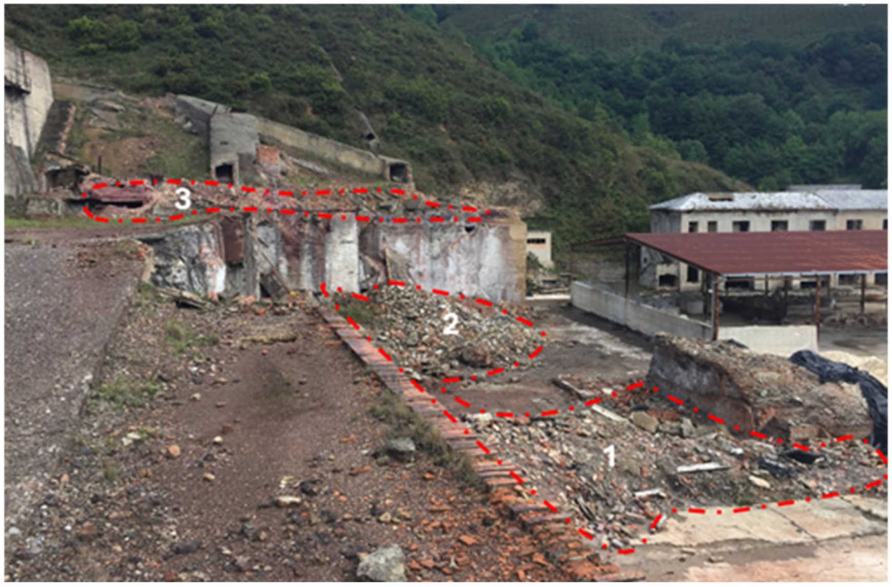
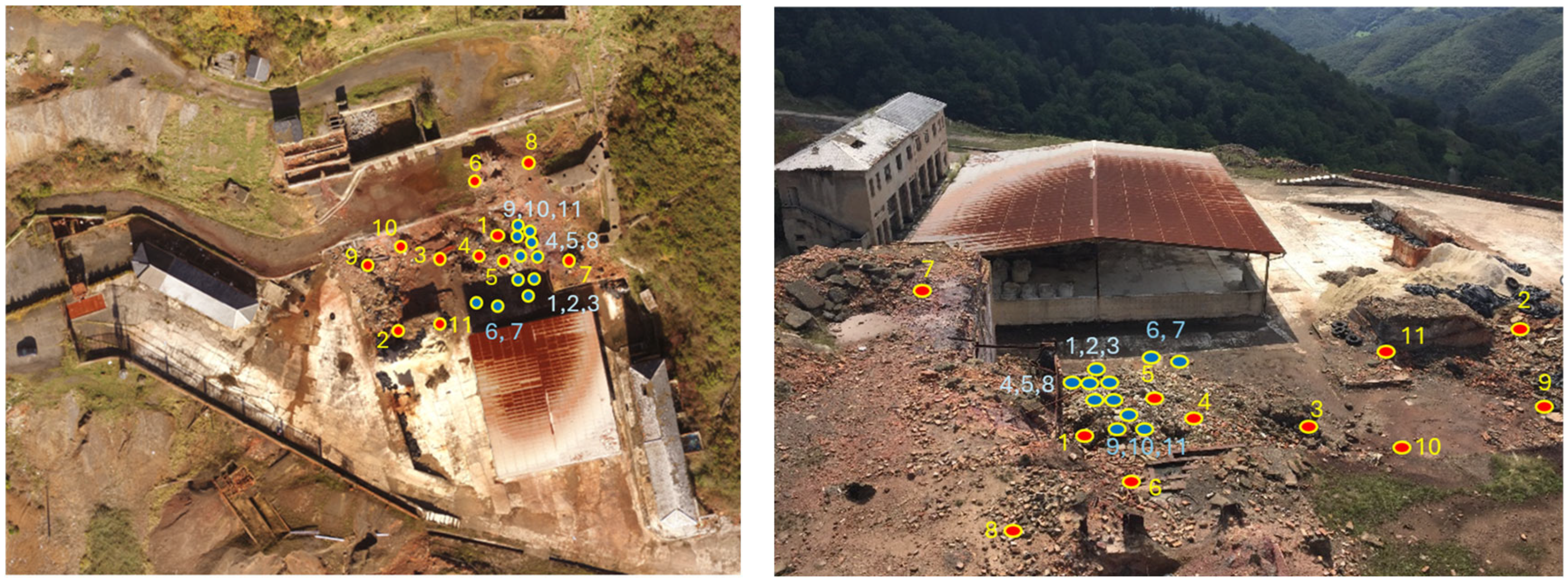
2.1. Abandoned Mercury Mining Facilities

This study was performed at the La Soterraña mining site composed of an underground mine and a smelting facility (Figure 1). The mineralization exploited in the La Soterraña mine is an epigenetic-type ore deposit that originated from low-temperature hydrothermal solutions. The paragenesis of the ore deposit is constituted by cinnabar, orpiment, realgar, pyrite (usually with high concentrations of As), arsenopyrite, marcasite, and pararealgar, in a gangue of quartz and calcite. Native Hg has been observed to be associated with organic matter-rich limestones [24]. Mercury ore was extracted using a room and pillar method and, subsequently, processed and recovered at the surface installations from the 19th century up to the 1970s. Afterward, the complex was abandoned without morphological restoration or any preventive measure to avoid mercury contamination. The metallurgical plant buildings were demolished in 1989 and debris from the demolition, which has a high mercury content [29], remained on site (Figure 1). It is a heterogeneous waste, a mixture of demolition debris from the buildings and concrete structures that supported the roasting furnaces, while the other waste is found in chimneys and ducts (dust, soot, etc.).

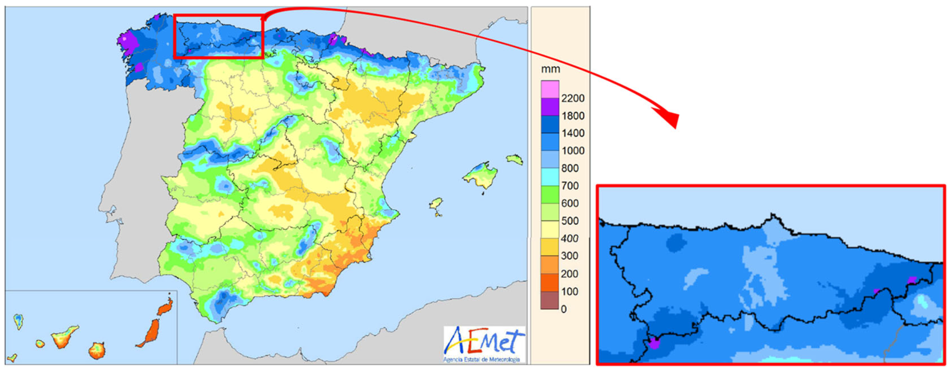
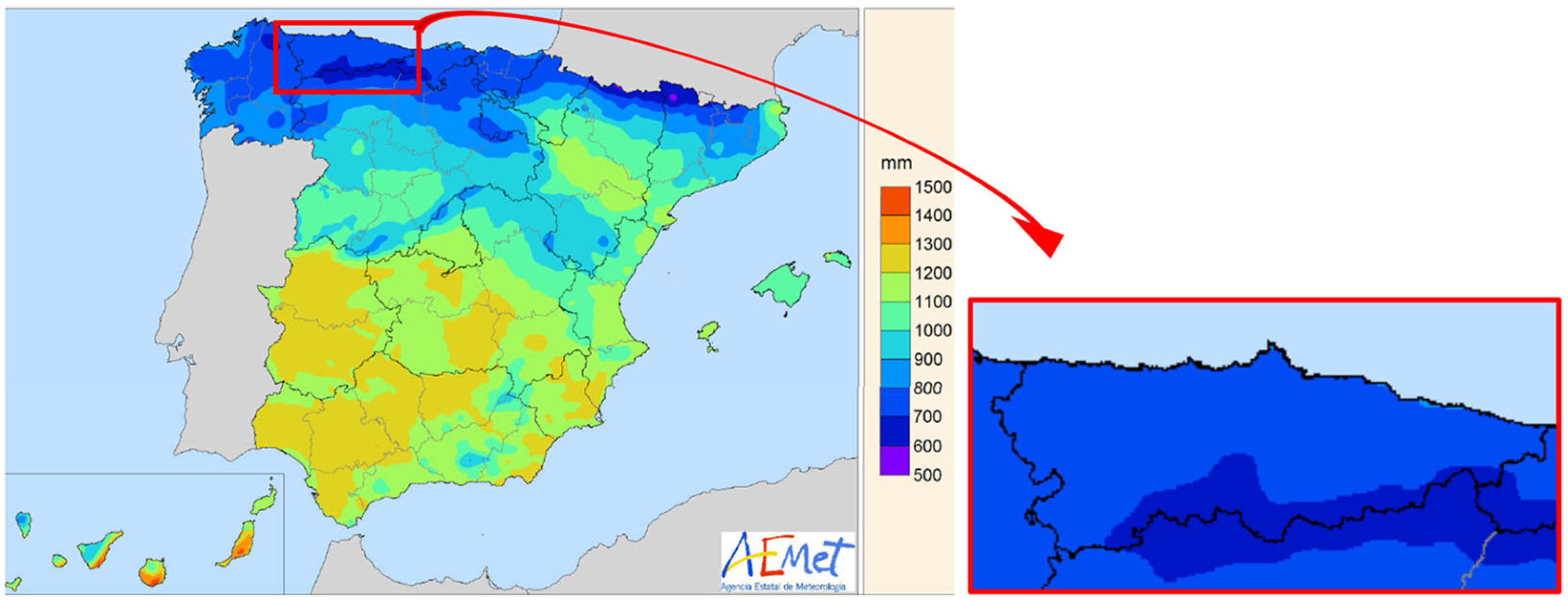
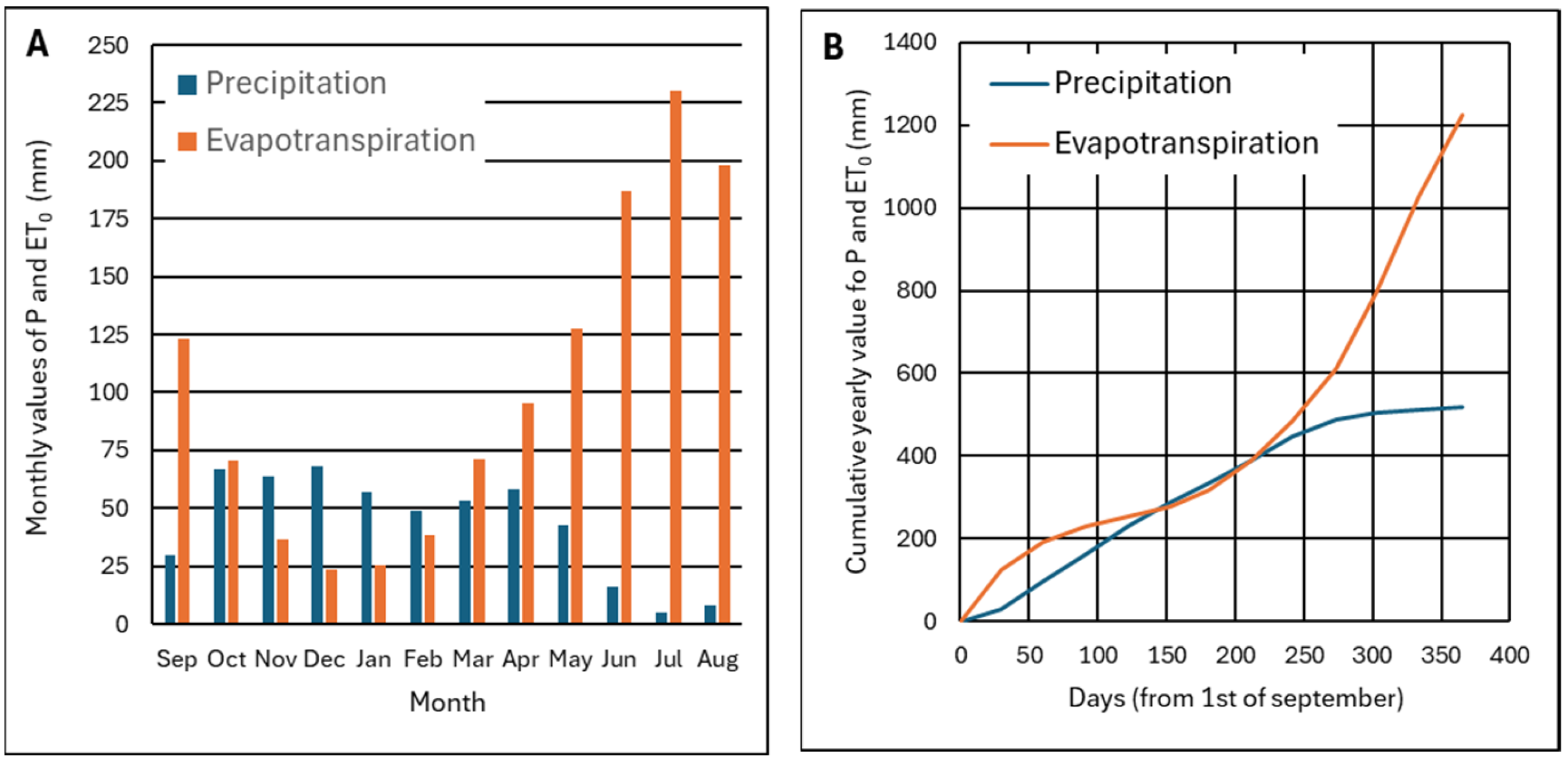
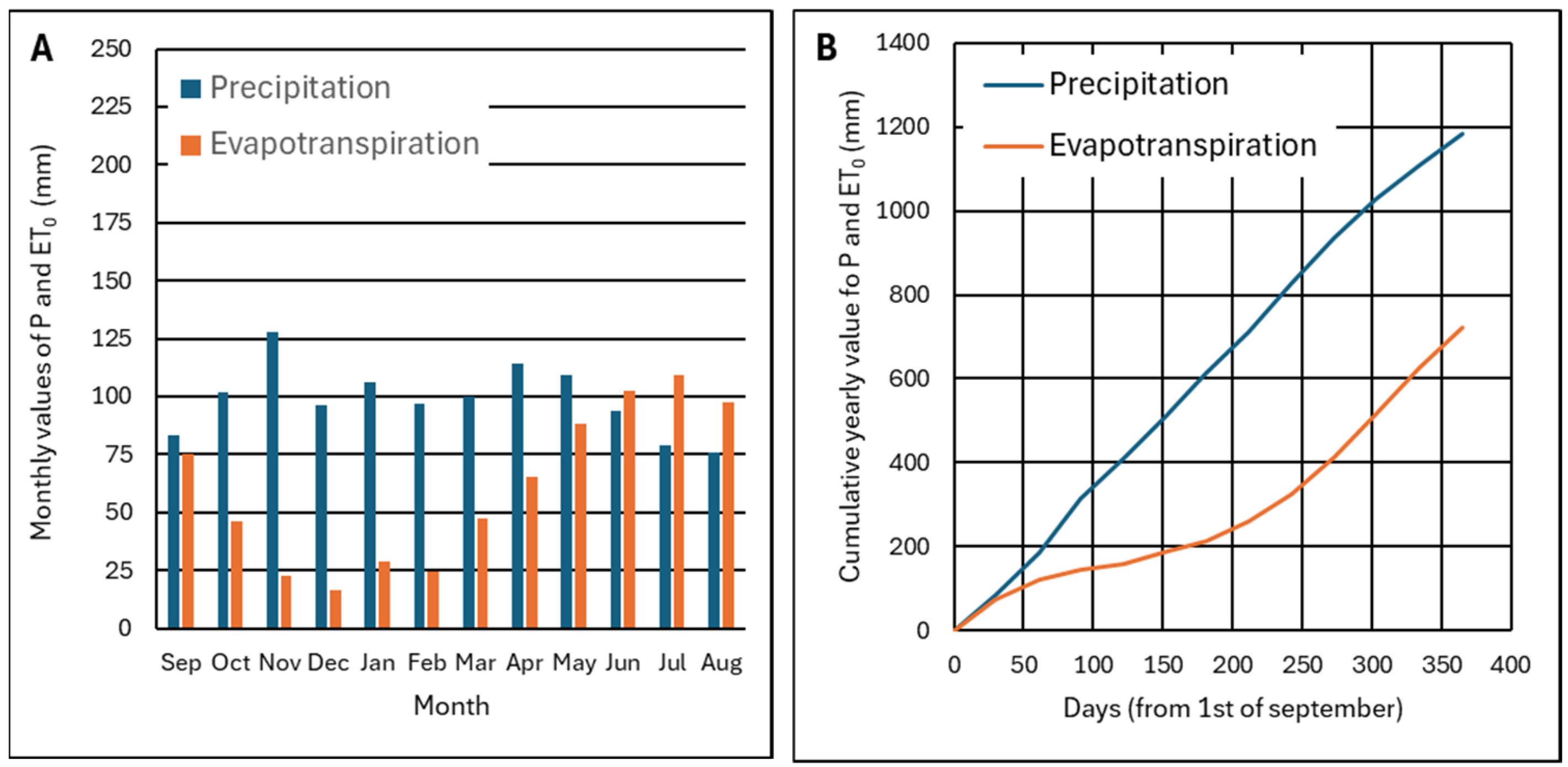
2.2. Precipitation and Evapotranspiration in the Study Area

Figure 2 shows a map of Spain with the location of Asturias. The average annual rainfall in Asturias is about 1200 mm/year [30]. In the central area, where the particular case study is located, the average annual rainfall is somewhat lower, 800–1000 mm/year, while it reaches 1400–1800 mm/year in some mountainous areas of the Cantabrian Mountains (Figure 2). Consequently, evapotranspiration is low compared to other regions, with an annual average of about 700 mm/year [31]. In the central area is slightly higher, 700–800 mm/year, while, further south towards the Cantabrian Mountains, it decreases to 600–700 mm/year (Figure 3). As can be seen, the precipitation P and evapotranspiration ET₀ are quite balanced in the area studied, with the ET₀/P ratio being close to unity.

2.3. Rainwater Contamination

One of the more serious problems in sites highly contaminated with mercury and arsenic is the contamination of rainwater producing leachates with a high concentration of mercury and arsenic. As has been said before, in the studied area, there was heterogeneous waste formed on one side by the waste produced in the demolition of structures, and on the other side, by the waste remaining in roasting furnaces, chimneys, and ducts like dust, soot, etc. In the following, we will use waste or debris indistinctly to denominate this mixture. Before building the treatment cell, this waste occupied three different zones of about 200 m² each, as it is shown in Figure 4. In zones 1 and 2, both on the lower platform, there was waste related to structures that supported the roaster, while in zone 3, on the upper platform, there was waste related to several ducts to the chimneys.

A total of 11 solid samples were taken: 4 in zone 1, 4 in zone 2, and 3 in zone 3. The distribution was approximately uniform, and sampling was carried out by taking samples of every type of waste. To build the treatment cell, the waste of zone 1 and, partially, the waste of zone 3 were moved to zone 2. This mixture of waste was later put in the treatment cell and covered with ashes. Consequently, the 11 solid samples could be considered representative of the heterogeneous waste of zone 2, which was finally treated.

On the other hand, 11 leachate samples were taken in zone 2 during a rainy period after collapsing the wall and mixing the debris.

Figure 5 shows the location of the 11 solid (red) and 11 leachate (blue) sampling points. It must be considered that solid and leachate samples were not taken at the same time. Nevertheless, the time elapsed between solid sampling and leachate sampling was only a few months, and no significant changes in the solid materials occurred.

The sampling procedure was the same as followed in previous studies, including from Ayala and Fernández [32]. Samples of waste of about 0.5 kg were taken in the study area. The waste was dried at room temperature in order to minimize the loss of volatile contaminants. Then, it was crushed using a jaw crusher and subsequently sieved through a 2 mm aperture screen before use. A fraction of the solids was milled to a particle size of <100 μm to determine the chemical composition and pH.

Liquid samples of 10 cm³ were taken from runoff water or water accumulated in puddles within the debris area. The water samples were introduced in tubes adding Hg-free acid and stored in a refrigerator until the analysis.

X-ray fluorescence (Phillips PW2404) was used to determine the major elements, while the quantification of the trace elements was performed by mass spectrometry with inductively coupled plasma (ICP-MS Agilent 7700, Agilent Technologies, Santa Clara, CA, USA) prior to dissolution with aqua regia using an Anton Paar 3000 microwave system, Ostfildern-Scharnhausen, Germany.

The pH value of the samples was measured using an Eutech pH 2700 m, Euthec, Syngapore) in a 1:2.5 (w/v) sample/water mixture after equilibrating for 30 min. In addition, the content of dissolved Ca, Mg, and Fe in the supernatant liquid from the byproducts was determined by atomic absorption spectroscopy (Perkin Elmer AAnalyst 200, Shelton, CT, USA).

The mineral composition was analyzed by X-ray diffraction (PANalytical X′Pert Pro MPD with CuKα radiation, Malvern Panalytical, Malvern, UK). The diffractometer was operated at 45 kV and 40 mA, over the range of 2θ from 5° to 90°, with a detector speed of 1°/min.

The total arsenic present in the waste can be found in different forms: some are soluble in water (arsenate and weakly adsorbed species), soluble in Na₂HPO₄ (strongly adsorbed onto mineral surfaces), soluble in NH₄F (associated with Al oxyhydroxides), soluble in Na₄P₂O₇ (As bound to organic matter), soluble in ammonium oxalate/oxalic acid (As associated with amorphous Fe oxyhydroxides), soluble in bicarbonate and ascorbic acid (associated with poorly crystalline Fe hydroxide), and acid digestion in a microwave oven with HCl and HNO₃ (As coprecipitates with refractory minerals) [32].

Table 1. Concentration of As and Hg in solid materials and leachates.

Solid Sample	As (g/kg)	Hg (g/kg)	Leachate Sample	As (mg/L)	Hg (μg/L)
1	84.28	14.64	1	94.44	40.69
2	254.07	41.50	2	83.87	31.49
3	46.18	6.35	3	203.33	14.94
4	54.80	34.69	4	160.98	14.34
5	44.42	7.49	5	137.82	10.14
6	44.12	22.19	6	188.63	8.47
7	29.64	19.05	7	246.11	8.03
8	603.34	25.29	8	820.38	12.88
9	210.00	16.00	9	732.89	12.24
10	48.00	0.53	10	571.92	16.05
11	98.59	1.45	11	332.06	12.51
N	11	11	N	11	11
Min	29.64	0.53	Min	83.87	8.03
Max	603.34	41.50	Max	820.38	40.69
Average	136.13	17.20	Average	324.77	16.53
SD	172.07	13.17	SD	261.85	10.20

provides the analysis results of the 11 samples and the representative statistical values for the concentration of arsenic and mercury in the soil and in the leachate produced. Extremely high concentrations of As and Hg are related to stupp and soot from roasting furnaces and flue dust in chimneys. The biggest As concentration in sample 8 could be considered unrealistic due to an error during sampling or laboratory analysis. Nevertheless, even if sample 8 is not considered in the calculation, the average concentration of As and Hg are 89.41 and 16.39 g/kg, which can also be considered extremely high.

An analysis of a representative sample of this waste was carried out in [32] in which the physical–chemical characteristics were determined (

Table 2. Chemical composition of waste after Ayala and Fernández [32].

SiO2 (wt%)	61.7	Hg (mg/kg)	34,691
Fe2O3 (wt%)	7.1	As (mg/kg)	54,801
MgO (wt%)	-	Zn (mg/kg)	0.03
K2O (wt%)	0.8	Cu (mg/kg)	420
Al2O3 (wt%)	7.1	Cr (mg/kg)	920
CaO (wt%)	3.9	Pb (mg/kg)	3400
SO3 (wt%)	7.2	Ni (mg/kg)	0.02
TiO2 (wt%)	0.55	Cd (mg/kg)	0.01
MnO (wt%)	0.02	pH	5.1

). In the present study, we focused only on mercury and arsenic.

A characteristic of this debris is its ability to produce contaminated leachate. When a water flow comes into contact with them, some of that arsenic and mercury passes into the water, producing the leachate. This has been observed during rainy periods. For example, after 2 weeks of heavy rain where 115.4 mm accumulated over 14 days, with an average temperature of 8.4 °C during the period, a water sample was taken from a rain puddle formed on the debris. The arsenic and mercury concentrations in the water reached 203.33 mg/L and 14.94 µg/L, respectively. Subsequently, the rainfall decreased, and a week later (with a more moderate precipitation of only 15.0 mm), the arsenic and mercury concentrations in the puddle varied inversely. While arsenic concentration increased to 246.11 mg/L (possibly due to water evaporation), the mercury concentration decreased to 8.03 µg/L (for example, due to precipitation), from which is inferred that the rainy/dry periods influence.

This contamination is practically instantaneous; the water does not need to be in contact with the debris for a long time, and it can reach much higher contamination levels after periods without rain. Due to drought conditions, a test was conducted in July, where the debris had to be watered with simulated rainwater. At that time, the debris was completely dry. Over the last two weeks, the average temperature had been 20.3 °C, and the accumulated rainfall had only reached 3.8 mm, with the peculiarity that it did not rain on the previous 5 days. The water was in contact with the debris for only a few minutes, yet the arsenic concentration in the water reached 94,436 and 83,867 µg/L, and the mercury concentration reached 40.69 and 31.49 µg/L. These values are in accordance with some tests carried out in the laboratory [32] in which the leachate obtained according to standard test [33] has a pH of 5.24, 196.8 mV redox potential, and 2.2 mS/cm conductivity. The analysis performed by mass spectrometry with ICP-MS shows a high content in As (59,056 μg/L) and much smaller amounts of Hg (0.98 μg/L), or other PTEs such as Ni, Zn, Cu, Cd, and Pb. About 1% of the arsenic present in the waste was solubilized during the test. Although the residue from mercury production has high concentrations of As and Hg, 54.80 g/Kg and 34.69 g/Kg, respectively, their mobility is small.

The average values of Hg concentration in both soils and leachates are in agreement with the results found by Vaselli et al. [34] for a large Hg mine site in central Italy.

3. Materials and Methods

3.1. Water Balance

The solution proposed, capping waste with ashes, is based on the hydraulic properties of fly ashes. It can be analyzed through the water balance in the soil represented by the following formula:

$$\mathrm{P}=\mathrm{E}+\mathrm{E}\mathrm{T}\mathrm{R}+\mathrm{R}+\mathrm{I}$$

(1)

P is the precipitation, the rainwater for a given period. A part of this rainwater does not penetrate in soil and becomes in the runoff E. Another part penetrates the soil, but it returns to the atmosphere as vapor through the actual evapotranspiration ETR. The remaining water is stored in the upper zone of the soil as recharge R. When this zone is saturated, the water begins to infiltrate I.

If the ashes have sufficiently high recharge capacity and sufficiently low permeability to facilitate evapotranspiration, then the water infiltration will be reduced and, consequently, it will not be contaminated. To analyze this process, a water balance model, which is described in detail in Appendix A, has been developed.

3.2. Tests’ Description

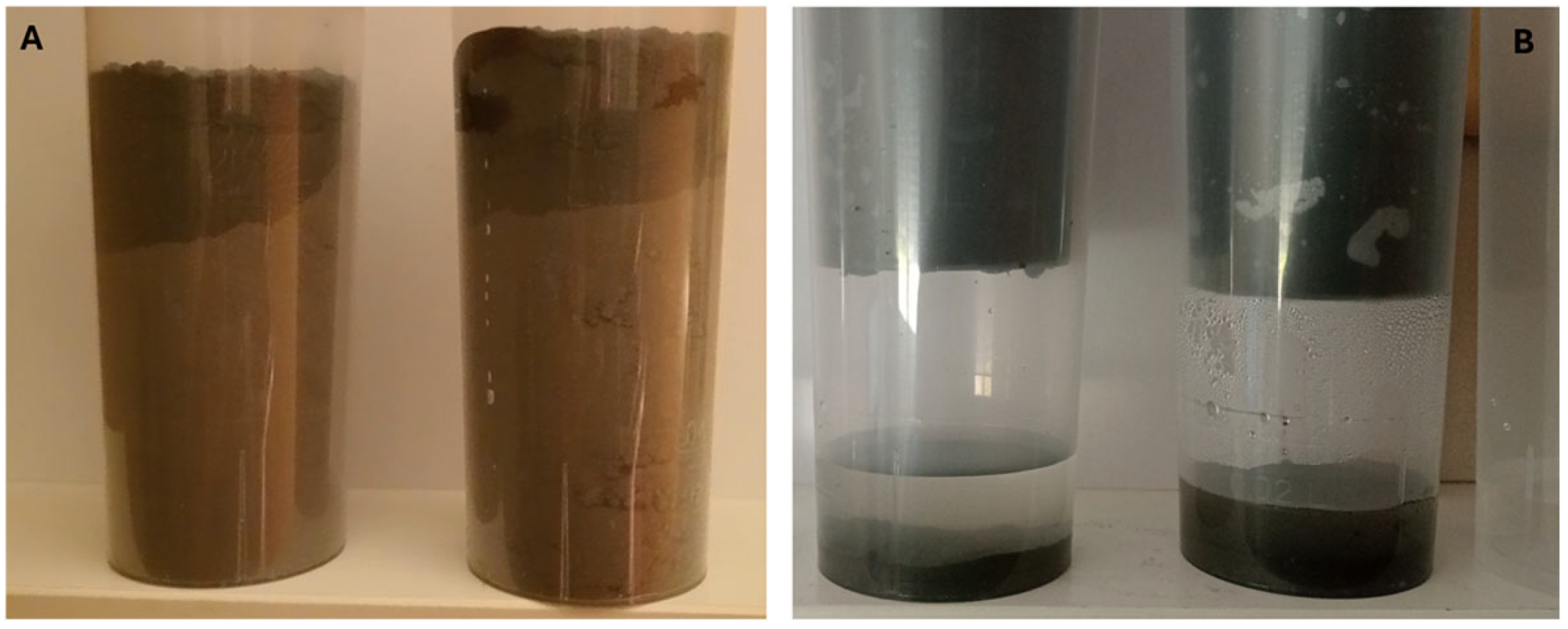
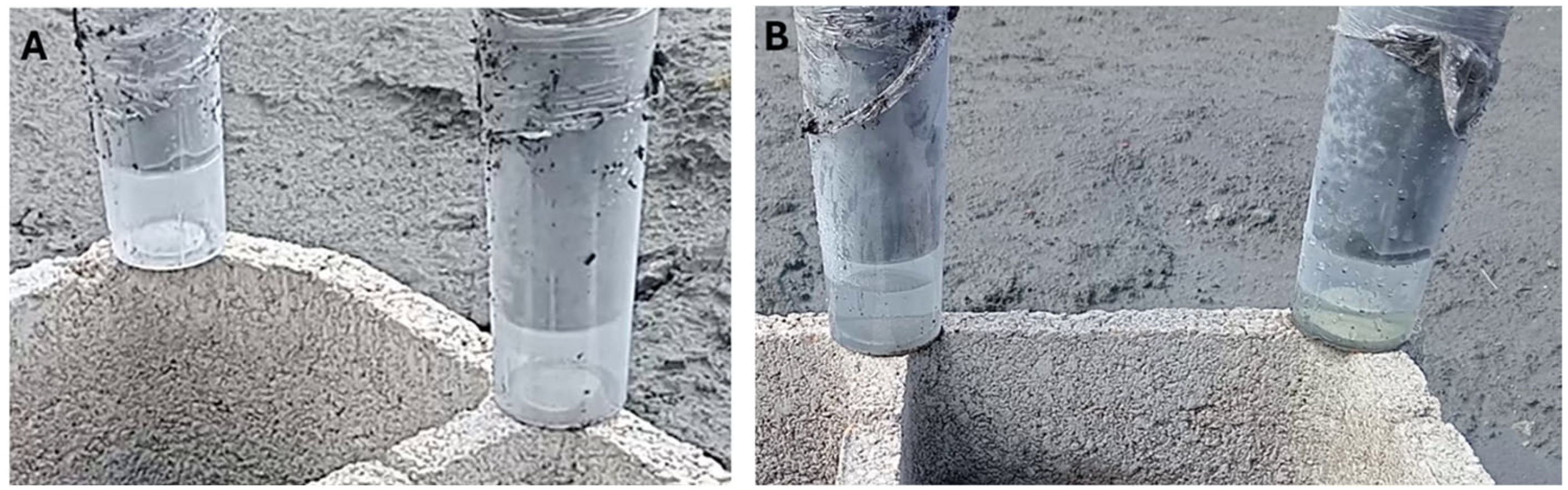
3.2.1. Laboratory Tests

The ashes used in this study come from a conventional coal-burning power plant, which uses hard coal, more concretely, subbituminous coal. Physical and chemical properties were determined from laboratory tests. The chemical composition of ashes was determined and presented in another work previously [33].

Table 3. Chemical composition of fly ash used in the study after Ayala and Fernández [32].

SiO2 (wt%)	56.5	Hg (mg/kg)	2
Fe2O3 (wt%)	9.5	As (mg/kg)	59
MgO (wt%)	0.9	Zn (mg/kg)	90
K2O (wt%)	2.61	Cu (mg/kg)	57
Al2O3 (wt%)	23.9	Cr (mg/kg)	83.6
CaO (wt%)	3.4	Pb (mg/kg)	16
SO3 (wt%)	2.04	Ni (mg/kg)	65.4
TiO2 (wt%)	0.85	Cd (mg/kg)	1.84
MnO (wt%)	-	pH	10.9

summarizes the results.

However, in this case, the ashes are studied as soil capable of retaining moisture from rainfall, a use that is different from the other uses given above. Laboratory tests have been carried out to determine those characteristics that influence the ashes’ capacity to absorb water and store it up to a limit (porosity recharge) and to transmit water at a constant flow rate (hydraulic conductivity).

Table 4. Physical properties of the ashes used in the study.

Parameter	Value	Standard
Bulk density (g/cm3)	0.96	[35]
Actual particle density (g/cm3)	2.38	[36]
Moisture content of the ash in stockpile (% by weight)	1.24	[37]
Porosity (% by volume)	58.8	[35]
Hydraulic conductivity (m/s)	2.83 × 10−6	[38]

shows the results.

It should be noted that the determination of the porosity is made by raising the temperature to 106 °C. However, under normal conditions of ash deposition as supplied by the thermal power plant, the ash has a very low moisture content, in the order of 1.24% (by weight). Therefore, assuming normal conditions in which the stockpiled ashes are protected from rain, the humidity will always be very low, and we can take this value as a reference. An amount of 1.24% by weight is approximately equivalent to 3.0% by volume. That means that the maximum value of porosity to be considered under normal conditions will not be 58.8% (by volume), but approximately 55.8% (by volume), since there is 3% moisture that is always present in the ash.

The value of both the physical and chemical properties is within the range for this type of coal according to previous studies that compared ashes from different power plants in Spain [39,40].

Given the ease of determining the properties of interest, scale experiments were also carried out, which were very useful and provided great information since they could be carried out both in the laboratory and in the field.

In the laboratory experiments, transparent plastic test tubes with a diameter of 5 cm were used. Depositing 200 g of dry ash in it (with 1–2% humidity, as supplied by the thermal power plant). This amount of ash reaches a height of about 10 cm, which, as will be justified later, is the height taken as a reference. Water was then added, observing how it penetrated the ash and slowly descended, as shown in Figure 6A. The process was repeated until it was saturated with water. At this point, water began to flow from the bottom and the constant flow rate through the test tube was measured, as in Figure 6B.

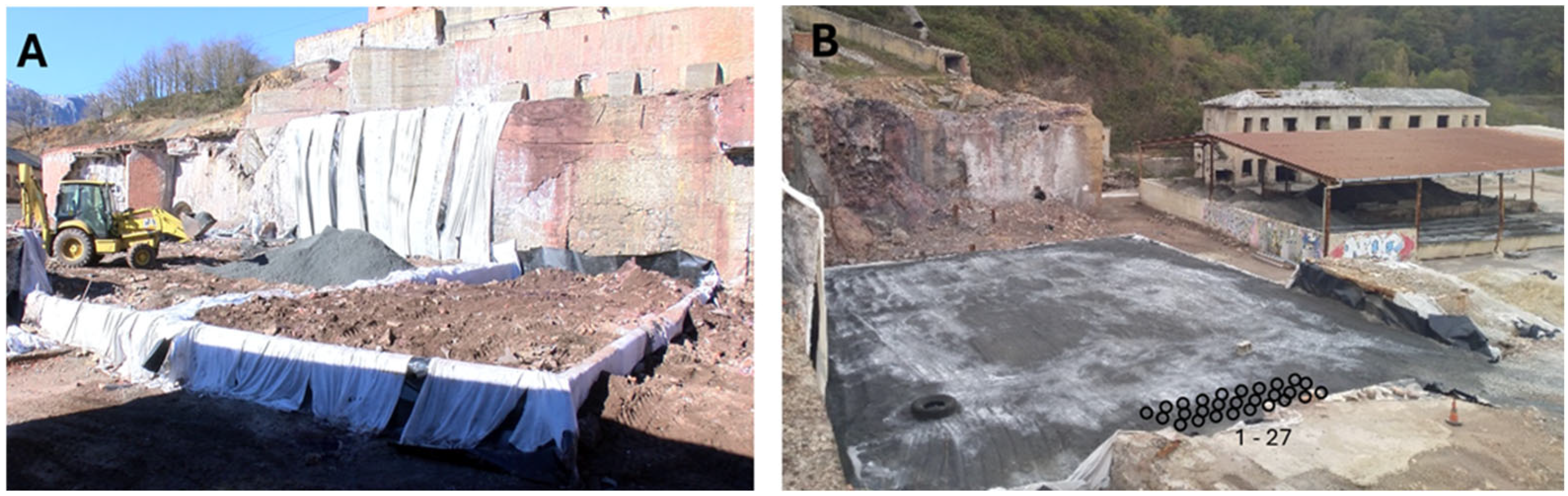
3.2.2. Full-Scale Tests in the Abandoned Mine Facilities

In addition to the laboratory tests, it was necessary to carry out a full-scale test to check the behavior of fly ash in the real conditions in which it is applied.

The rubble was removed to build the impermeable cell and then relocated inside it (Figure 7A). The cell was a pool of 600 m² limited by the high walls that previously existed and new small concrete walls of 1.20 m high (Figure 7B). The work was carried out under very risky conditions, because the Hg concentration in the air was very high, and a safety protocol for working in this area had to be developed by Rodríguez et al. [29].

Fly ashes are considered not to be dangerous waste and slags are considered an inert material, following Spanish legislation, and their use is common in civil works for road filling or road slopes. Both by-products were characterized to avoid the introduction of a new concern for the local environment: the concentration of Hg and As in these by-products was negligible in comparison with the demolition waste [32]. On the other hand, companies that supply by-products have experience in managing large landfills in which these by-products are deposited; consequently, their potential effects on the environment, of very low intensity, are well known.

As described by Rodríguez et al. [29], the ash coating was effective in stopping mercury emissions into the air. Even in the same work, it was reported that it prevented water contamination. Nevertheless, the factors that influence water infiltration (ash permeability and porosity and some climatic conditions) are studied in depth in the present work.

Field data collection was conducted for three months, from 4 April 2024 to 4 July 2024, which can be considered a normal rainfall regime (95% of the average of the last ten years, after AEMET). Several variables were measured directly in the field (Figure 8). Precipitation was measured by direct reading in a rain gauge. Solar radiation was deduced from ultraviolet radiation directly measured with a portable Photo-radiometer HD2102.1 with a sensor LP 471-PA from DeltaOhm manufacturer, Casselle di Selvazzano, Italy. Ambient temperature was measured with a conventional thermometer or by temperature sensors Sensit TG8 Pt 1000/3850, Ostrava, Czech Republic, coupled to a Comet datalogger, Comet Systems, Roznov pod Radhostem, Czech Republic. With these variables, evapotranspiration can be empirically determined (using Turc’s law or similar), and, together with the precipitation, the theoretical water balance in the ashes can be empirically established.

On the other hand, samples of the ash coating were periodically taken for moisture determination (Figure 9). In this case, it was important for the ashes to become saturated in water with the normal level of precipitation during these months. Therefore, a small area was prepared by reducing its thickness to only 100 mm thick (Figure 7B). A total of 27 ash samples were taken. Samples consisted of 33 mL of ash and between 3 and 5 samples were taken at different depths between 0 and 100 mm. Ash samples were dried at room temperature and then the wetness was determined as described above.

The ash wetness allows us to establish the actual water balance that took place in that soil and can be compared with the prediction made from other variables.

The mechanism by which the actual infiltration occurs, once the ashes are saturated in water, is related to the hydraulic conductivity of the ashes. To study this process in more detail and to be able to compare it with what was observed in the laboratory, several specimens equal to the one in the laboratory were buried in the ashes (Figure 10). Half of the specimens were filled with completely dry ashes while the other half were filled with wet ashes from the site itself.

Since the issue of water balance is very important for agriculture, all countries have their meteorological agencies that provide very reliable data on the variables of interest. For this reason, to take all the information available from these agencies is recommended. In this case, day by day, AEMET provides the following variables registered in the station of Rozón (Lena), a few kilometers away from the study area:

• Summary of precipitation, temperature, etc., hour by hour.
• Summary of precipitations, temperatures, etc., of the previous days.

In addition to this, every ten days, it issues a bulletin on the water balance that already gives a value of the accumulated evapotranspiration during those ten days. The aim is to adjust with the data collected in situ a prediction model that, using the AEMET data, allows us to establish the water balance in the ashes that cover the debris.

In this way, this well-known methodology can be used at any site. It can be used directly where data from a meteorological agency are available, whereas the procedure previously explained should be followed if there are no in situ measurements.

4. Results

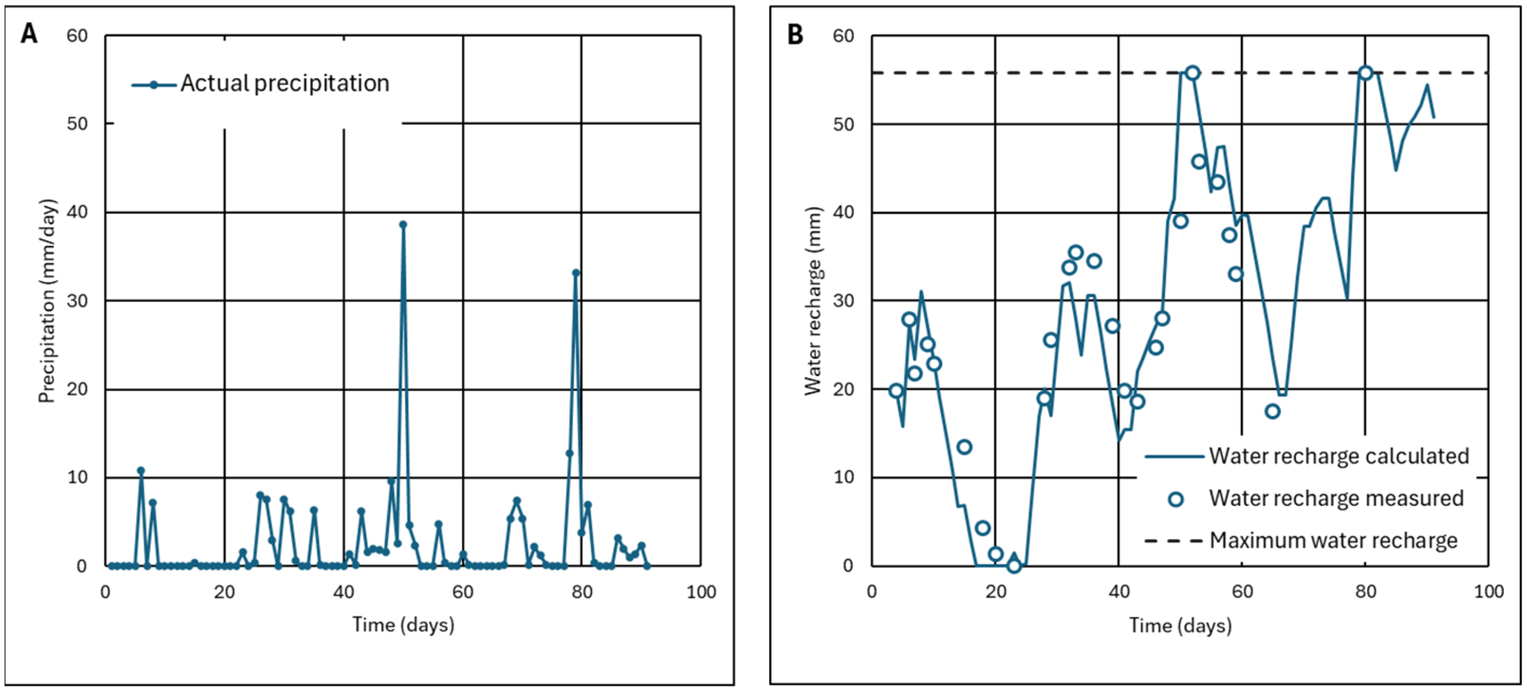
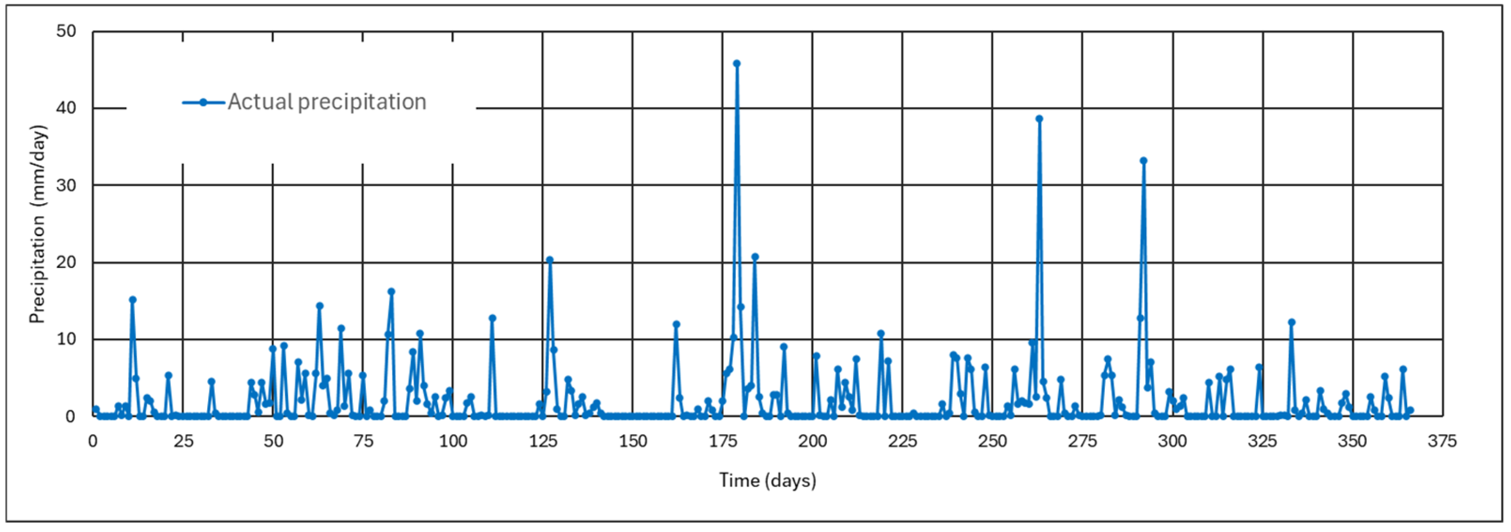
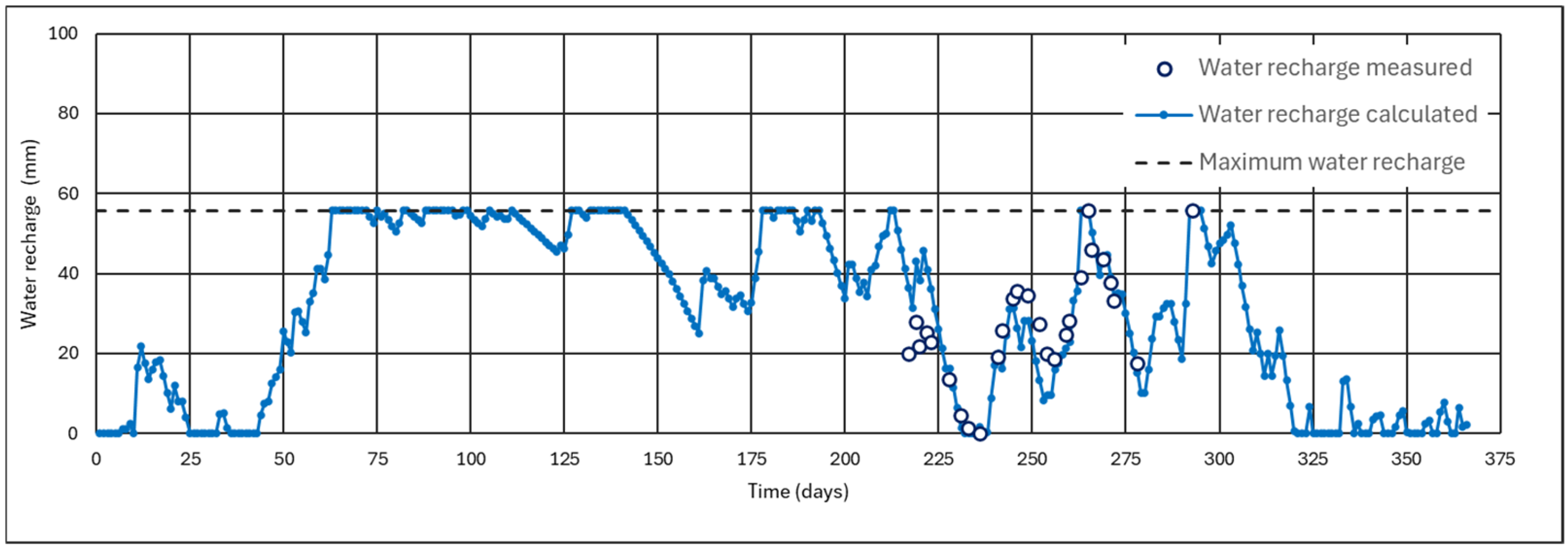
4.1. Results of the Tests in the Contaminated Debris Treatment Cell

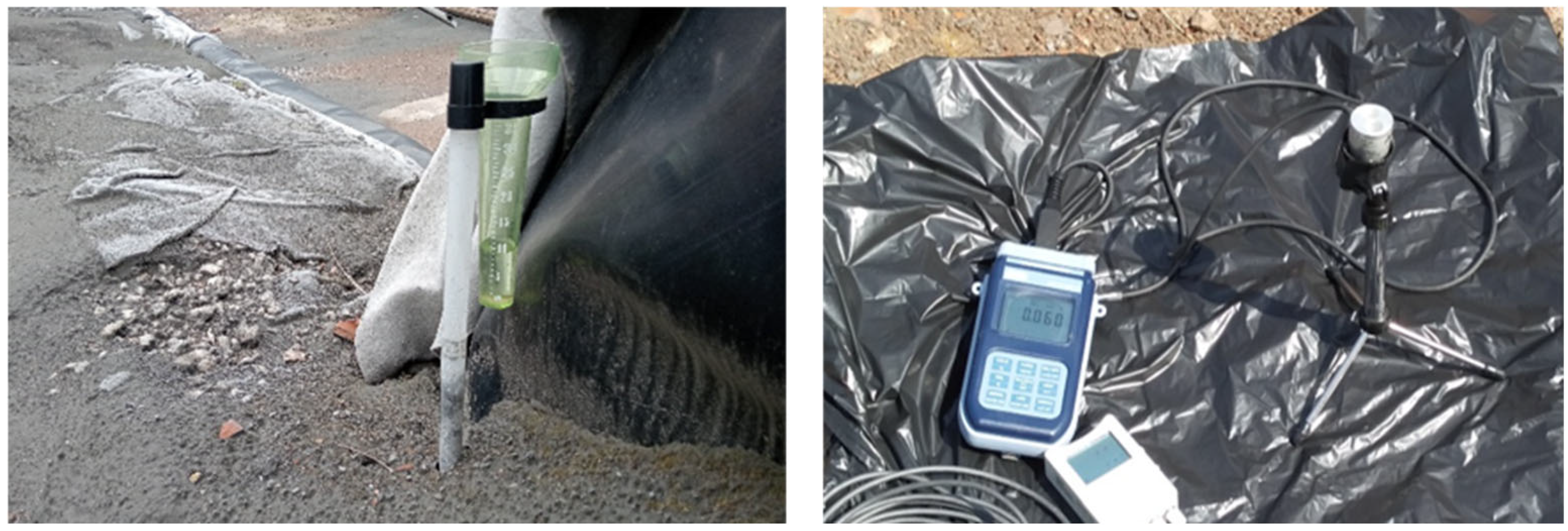
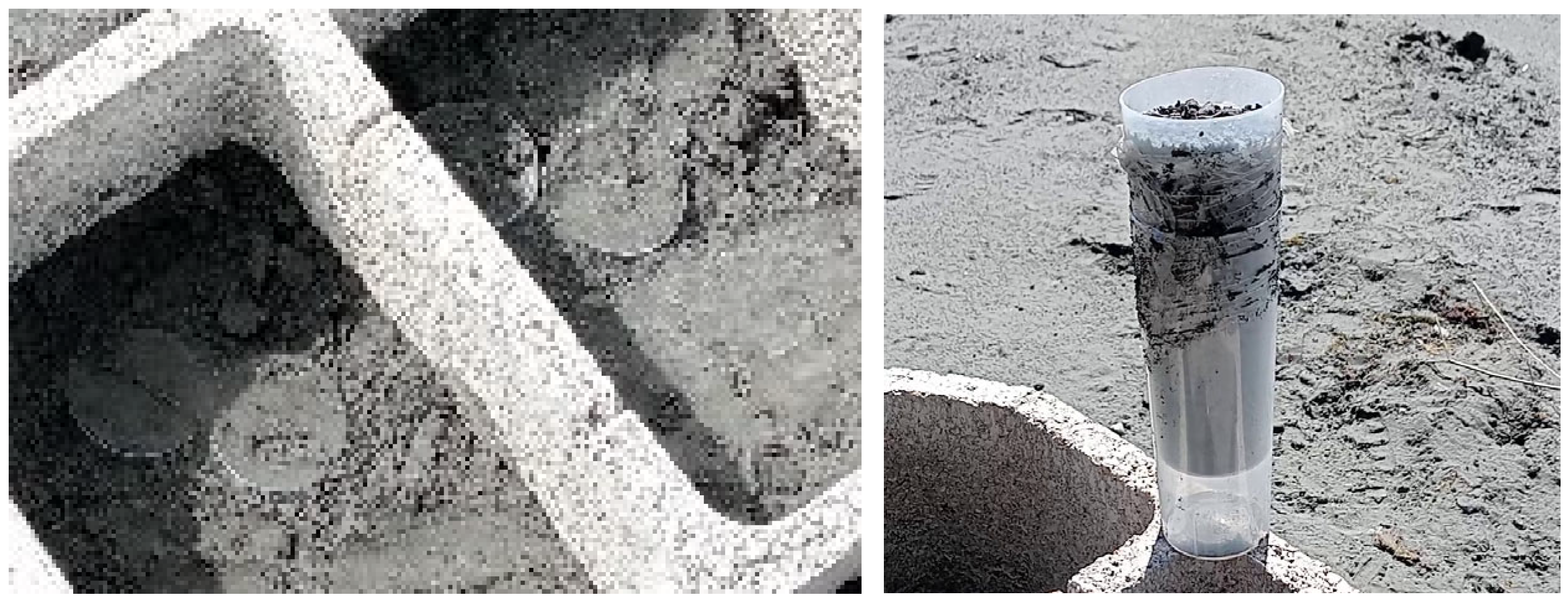
4.1.1. Results of the Monitoring of Ash Wetness for Three Months

The rainfall evolution is shown in Figure 11A. The data correspond to the Ronzón station, located about 10 km from the study area, which was tested with the direct reading in a rain gauge. In total, the precipitation recorded was 228 mm with an irregular distribution. It rained with an average of 3.5 mm/day approximately half of the days and there were two episodes of more intense rainfall, one with 38.6 mm/day and the other with 33.2 mm/day.

Figure 11B shows the evolution of water recharge in the ashes, which, as can be seen, is consistent with the rainfall distribution. The first measurement, taken after a week without rain, resulted in a recharge of 20 mm, slightly less than half of the maximum recharge. Thereafter, there is an increase in moisture in the ash due to several days of rain. Then, during two weeks without rain, the ash loses moisture until the recharge becomes zero. Subsequently, a new rain–no rain cycle causes the recharge to increase to 35 mm and decrease to 20 mm. The next is a rainy period in which recharge increases, reaching the maximum recharge (58.8 mm) on the day of maximum rainfall. This is followed by a period of low rainfall in which the recharge is again at 20 mm.

In the last month, only one control measurement was made after the second episode of heavy rainfall to verify that the ash has indeed been saturated again in water and has reached the maximum recharge. Figure 11B also shows the good fit obtained with the model (see Appendix A), which is able to predict the water recharge in the ashes on any given day.

On the day of the rainfall peak, 38.2 mm, the ash reached its maximum recharge and water began to pass through the ash, as demonstrated by the test specimens placed for this purpose. Until that day, no water had infiltrated (Figure 12A) while, from that day on, the ash became saturated and water started to pass through and was collected at the bottom, below the ash (Figure 12B). The volume of water collected was fully consistent with the calculations and the laboratory tests.

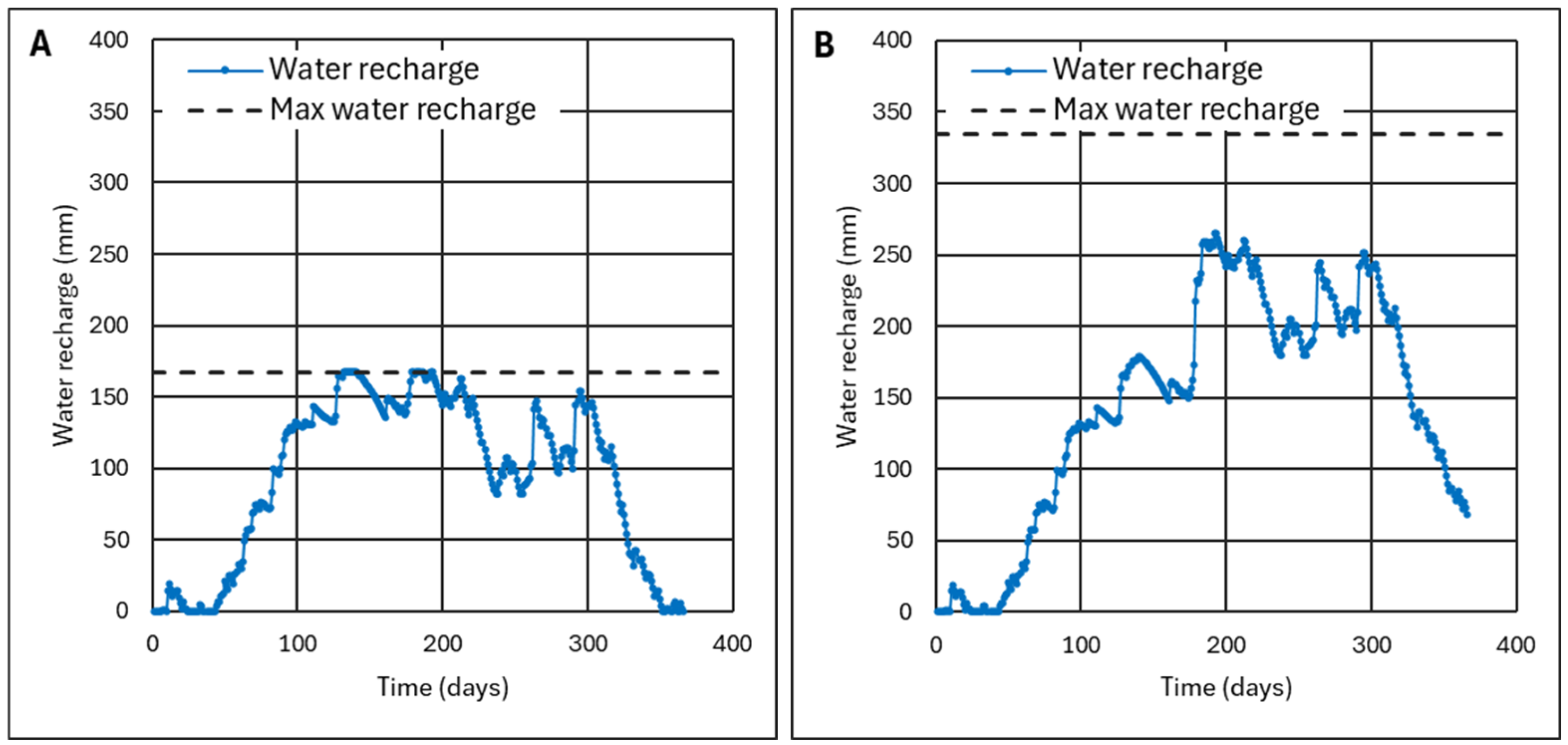
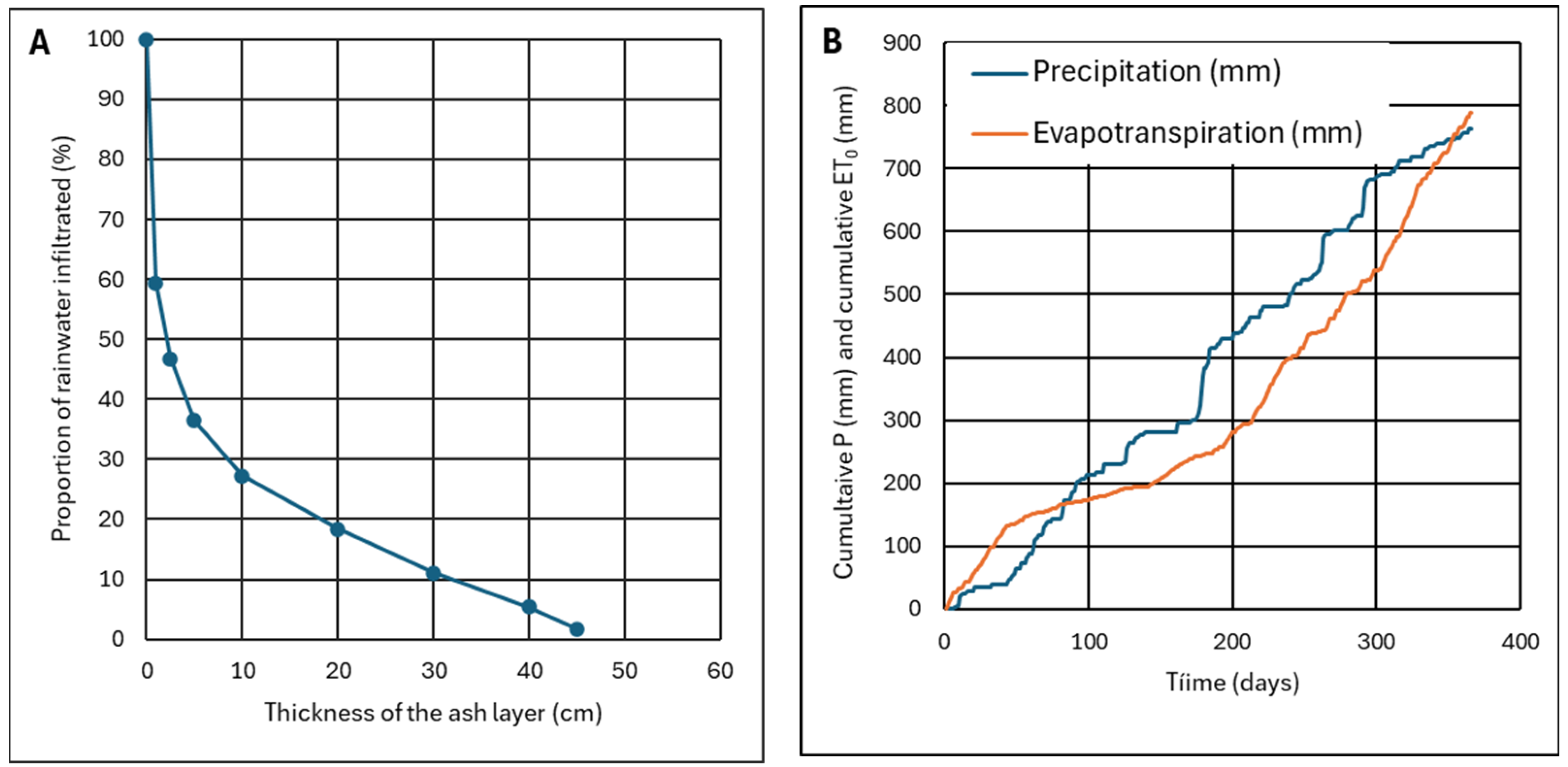
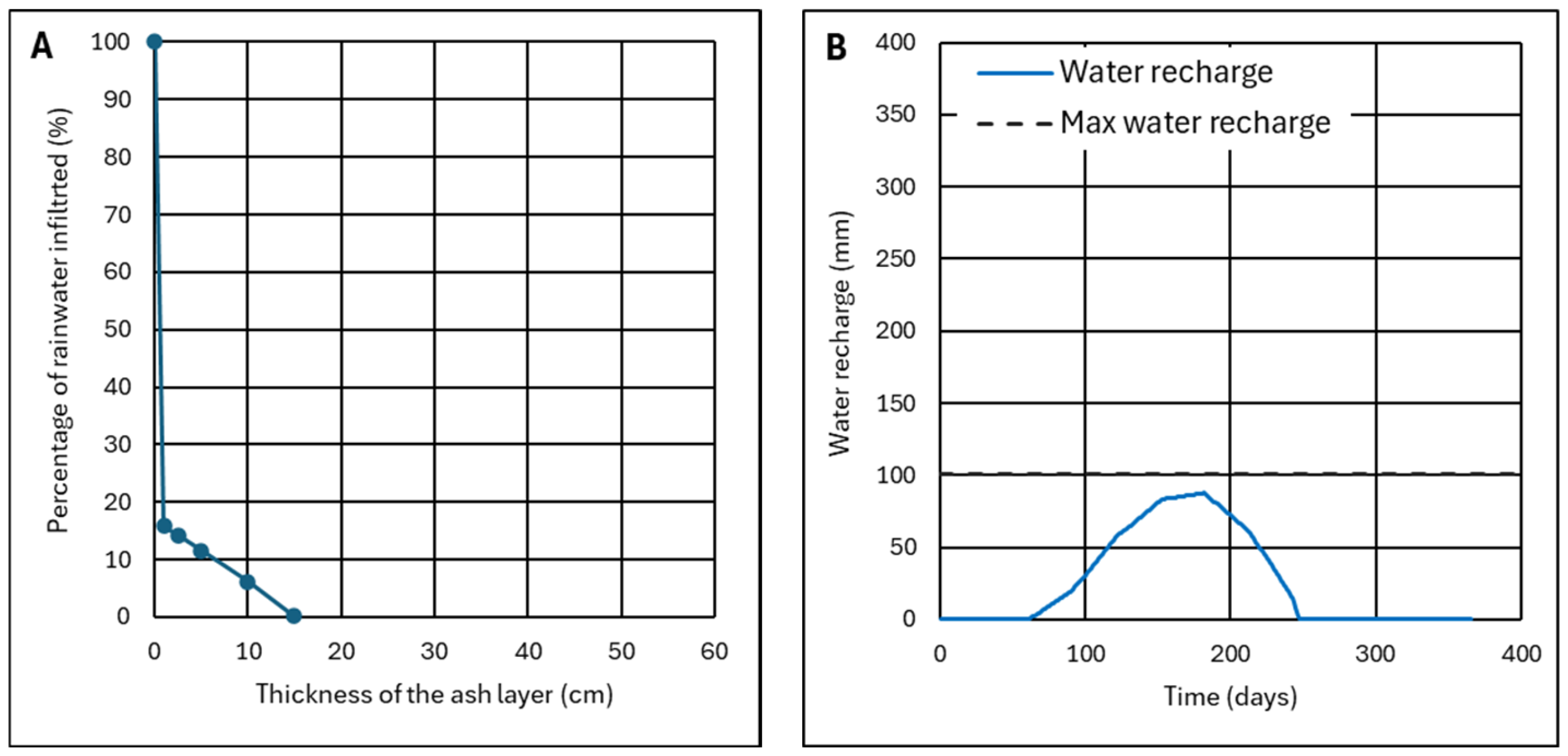
4.1.2. Effect of the Thickness of the Ash Layer

The thickness of the ash layer is crucial, since it will determine the proportion of rainwater that infiltrates and, therefore, becomes contaminated. The model developed can be used for this purpose. Having adjusted the model to predict the evolution of water recharge in the monitoring period, it is now of interest to predict the evolution of water recharge during a water year. The water year, which runs from September 1 to August 31 of the following year, is the complete natural cycle of rainfall at Spain’s latitude.

For this purpose, the model has been used with the temperature and precipitation data provided daily and the evapotranspiration data provided every ten days by AEMET, from 1 September 2023 to 31 August 2024.

Figure 13 shows the daily precipitation P (mm/day) throughout the year and Figure 14 displays the evolution of the water recharge in the monitored part 10 cm thick of the ash layer. It has been considered that on September 1, the beginning of the water year, the recharge was zero. This was contrasted with experience since August and September 2023 were dry months.

From November 15, it begins to rain regularly, and the ash becomes saturated with moisture, reaching the maximum possible recharge value of 55.8 mm. From then on, the rain contributes to maintaining the humidity until, as seen in the previous section, in April 2024 the recharge drops to zero because two weeks pass without rain. As seen in Figure 14, the model effectively reproduces the evolution of the water recharge.

In order to know if it is possible to find a layer thickness for which infiltration is zero, the model will be used with the data from the last hydrological year. By varying the thickness of the ash layer, the infiltration in each case is determined and an attempt is made to find a relationship. Given the infiltration process, two conditions must be met for the ash layer to not allow water to infiltrate:

• The ash layer must be thick enough so that the recharge does not reach the maximum recharge, which is the limit for start infiltration.
• The recharge, at the end of a hydrological year, must be zero or have the same value as at the beginning of this year.

Figure 15 shows two examples where one of the two conditions is not met. Figure 15A shows the evolution of water recharge when the thickness of the ash layer is h = 30 cm and the maximum recharge is 167 mm. Infiltration cannot be avoided because, at a given moment, the recharge reaches the maximum possible value, and water begins to pass through.

The thickness of the ash layer can be increased up to a point. Figure 15B shows how the variation in recharge never reaches the maximum recharge with an ash layer of h = 60 cm (maximum recharge of 334 mm). However, the recharge would be greater than 50 mm at the end of the water year, so it is not expected to be reduced to zero in the following months. A difference between evapotranspiration and precipitation of 50 mm would be required, which would be an anomaly in those months. On the other hand, both conditions are met for a layer thickness of approximately 40–50 cm.

The relationship between layer thickness and infiltration can be found by varying the layer thickness. As shown in Figure 16A, under the test conditions, a layer thickness as small as 10 cm (h = 10 cm) only lets through approximately 25% of the rainwater, preventing 75% of the rainwater falling on the treatment cell from becoming contaminated. In the optimum operation of the cell, a 40 cm layer would let through, at most, 5% of the water, and stop at 95%. It should be noted that, although the humidity control was carried out in an area with 10 cm of ash, the final average layer thickness in the cell was about 50 cm.

The fact that water does not infiltrate does not depend only on the characteristics of the ash, its permeability, and porosity, but also on the weather. Indeed, there must be a balance between evaporation and precipitation, seeking to at least balance them, as is the case study’s actual conditions. The explanation lies in the shapes of the precipitation and evapotranspiration curves accumulated over the year (Figure 16B). The ash layer only needs to have enough recharge to retain the excess rain if evapotranspiration is enough.

4.2. Analysis of Other Areas with Different Climatology

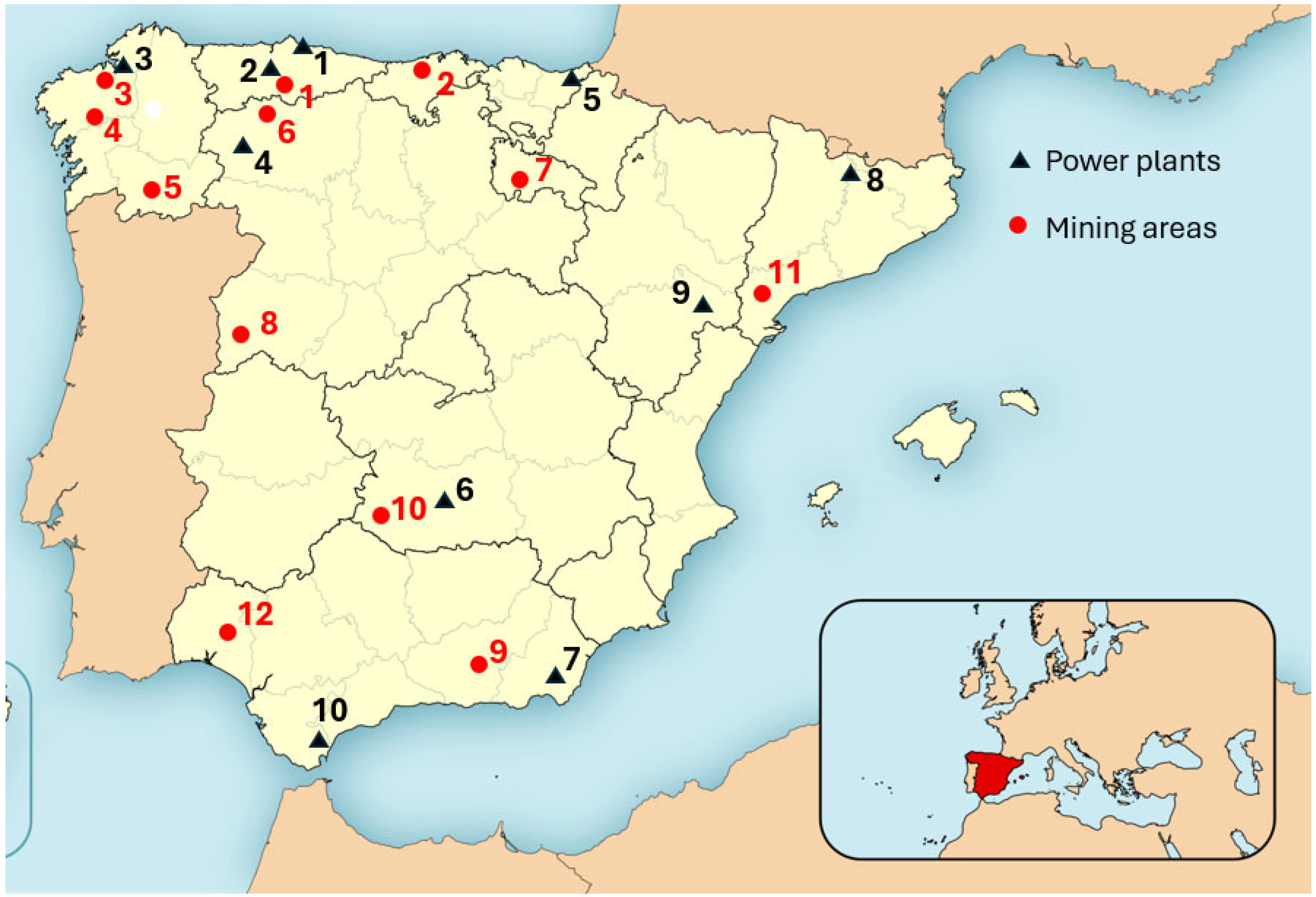
4.2.1. Selection of the Mining Areas

As seen in previous sections, the effectiveness of the solution of using thermal fly ash to cover contaminated soil or mining debris depends not only on the intrinsic characteristics of the ash but also on the weather. On the other hand, this solution has the advantage that it is independent of the contaminating elements, such as other metal mining sites, because it avoids direct contact with water.

Since meteorological agencies provide average annual data from different places in the country, an analysis of the effectiveness of the solution can be made based on the weather. Several areas in Spain have been chosen that meet the following requirements:

• There has been metal mining in the past and there may be abandoned waste dumps that need to be restored.
• There could be future mining projects driven by the existence of strategic raw materials.
• They are less than 500 km from a thermal power plant (in operation or closed) with an ash dump.
• They have different climatic conditions from each other, with the evapotranspiration to precipitation ratio ET₀/P varying between 0.5 and 3.0.

Table 5. Basic data on mining areas.

Zone	Mineral	Location	Province	Power Plant	Distance
1	Mercury	Mieres	Asturias	Soto de Ribera (2)	15 km
2	Zinc	Torrelavega	Cantabria	Aboño (1)	162 km
3	Wolframio	Santa Comba	La Coruña	Meirama (3)	40 km
4	Copper	Santiago de Compostela	La Coruña	Meirama (3)	55 km
5	Tin, Wolframio	Beariz	Orense	Compostilla (4)	157 km
6	Iron	Villablino	León	Compostilla (4)	62 km
7	Lead	Santa Engracia	La Rioja	Pasajes (5)	190 km
8	Uranium	Ciudad Rodrigo	Salamanca	Puertollano (6)	481 km
9	Iron	Alquife	Granada	Carboneras (7)	149 km
10	Mercury	Almadén	Ciudad Real	Puertollano (6)	91 km
11	Arsenic	Bellmunt del Priorat	Tarragona	Cercs (8) Escatrón (9)	211 km 123 km
12	Copper, Silver	Riotinto	Huelva	Los Barrios (10)	258 km

gives the basic data and the location of the 12 mining areas, together with the 10 selected thermal power plants, is displayed in Figure 17. Since a general analysis is being carried out, annual mean data are used, which are, in turn, the average of several years [30]. The mean temperature and precipitation data correspond to the period of 1981–2010 and evapotranspiration corresponds to the period of 1996–2016. Evapotranspiration can also be estimated from solar radiation data [31] using Turc’s formula.

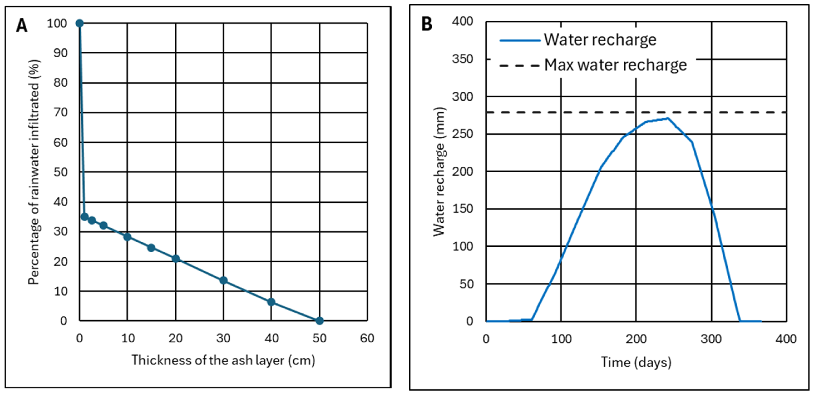
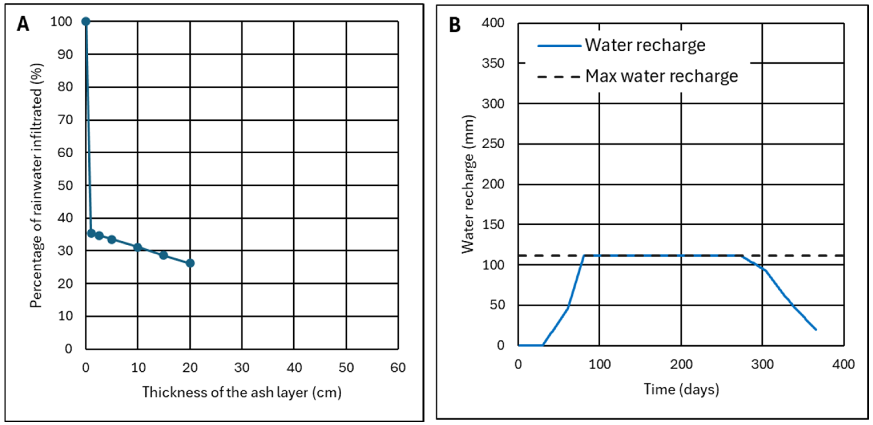
4.2.2. Analysis of Three Representative Cases

Based on the previous results, three cases have been selected that represent the main climatic scenarios that condition the behavior of the ashes and their waterproofing capacity. First, the Almadén mining district (zone 10) is analyzed, where the largest mercury mines in the world were exploited in the past. The predominant climate would be between the typical temperate climate, with dry and warm summers, and the corresponding cold steppe climate (Csa and BSk climates according to the Köppen classification). As can be seen in Figure 18A, rainfall is very moderate and there is a long period, more than half the year, in which evapotranspiration far exceeds precipitation. This means that while the accumulated precipitation, P, in a year, is just over 500 mm, the accumulated evapotranspiration ET₀ in the year reaches 1200 m (Figure 18B). The ET₀/P ratio is of the order of 2.4.

As can be seen in Figure 19A, 90% of rainwater infiltration is prevented with minimum layer thicknesses. From a layer of 15 cm onwards, water infiltration is zero because the ash retains all the water, and meteorological conditions cause its rapid evaporation (Figure 19B). Other areas similar to zone 10 are zones 9, 11, and 12 and, in them, the ET₀/P ratio is of the order of 2.0–3.0.

Another typical case is the mining area of Villablino (zone 6), where there was intense coal mining and also iron mining in the past. The climate is temperate, with dry and temperate summers (Csb according to Köppen). While in winter and spring precipitation exceeds evapotranspiration, in the summer–autumn period, the opposite occurs (Figure 20A). The result is a balance throughout the year that makes the accumulated precipitation in the year very similar to evapotranspiration, 800 mm, in both cases (Figure 20B). Consequently, the ET₀/P ratio is close to 1.

The characteristic of this zone is that 100% of infiltration is avoided, but a greater layer thickness is required (Figure 21A). Figure 21B shows the evolution of recharge with a 50 cm thick layer. Other zones similar to zone 6 are zones 5, 7, and 8. In them, the ET₀/P ratio is of the order of 0.8–1.2.

Finally, the last typical case is zone 2, where intensive lead and zinc mining took place. The climate is typical of humid Spain, temperate, without a truly dry season and with a mild summer (Cfb according to Köppen classification). Precipitation exceeds evapotranspiration practically all year (Figure 22A). Accumulated precipitation during the year, around 1200 mm, is much higher than evapotranspiration, around 700 mm, and evapotranspiration in the dry period is not enough to compensate for the humidity due to rainfall (Figure 22B). Under these conditions, the ash layer must be rather thin so that it can exhaust its recharge by the action of evapotranspiration. Figure 23A represents this fact by making the curve not cut the horizontal axis. However, it must be said that in the conditions of zone 2, a layer of only 20 cm (Figure 23B) allows less than 30% of the rainwater to infiltrate, preventing 70% of it from becoming contaminated. Zones 1, 2, 3, and 4 are similar, with the ET₀/P ratio < 0.8.

4.2.3. Criterion to Determine the Ash Layer Thickness for Minimum Infiltration

The previous analysis allows the establishment of a criterion that can be used as a first approximation to evaluate the suitability and limits of using an ash layer to cover an area contaminated with PTEs to prevent the contamination of rainwater.

The intrinsic properties of ash, permeability and porosity, do not fully determine the result, requiring the climatological variable to be considered. As can be seen in Figure 24, the ET₀/P ratio can be used as a representative variable of the climate, where ET₀ is the evapotranspiration and P is the precipitation accumulated in the year. Figure 24A can be used to determine, approximately, the thickness of the ash layer h_u (cm) necessary to reach minimum infiltration. Additionally, Figure 24B gives the value of the minimum infiltration expected I (%).

Based on these results, the following can be stated:

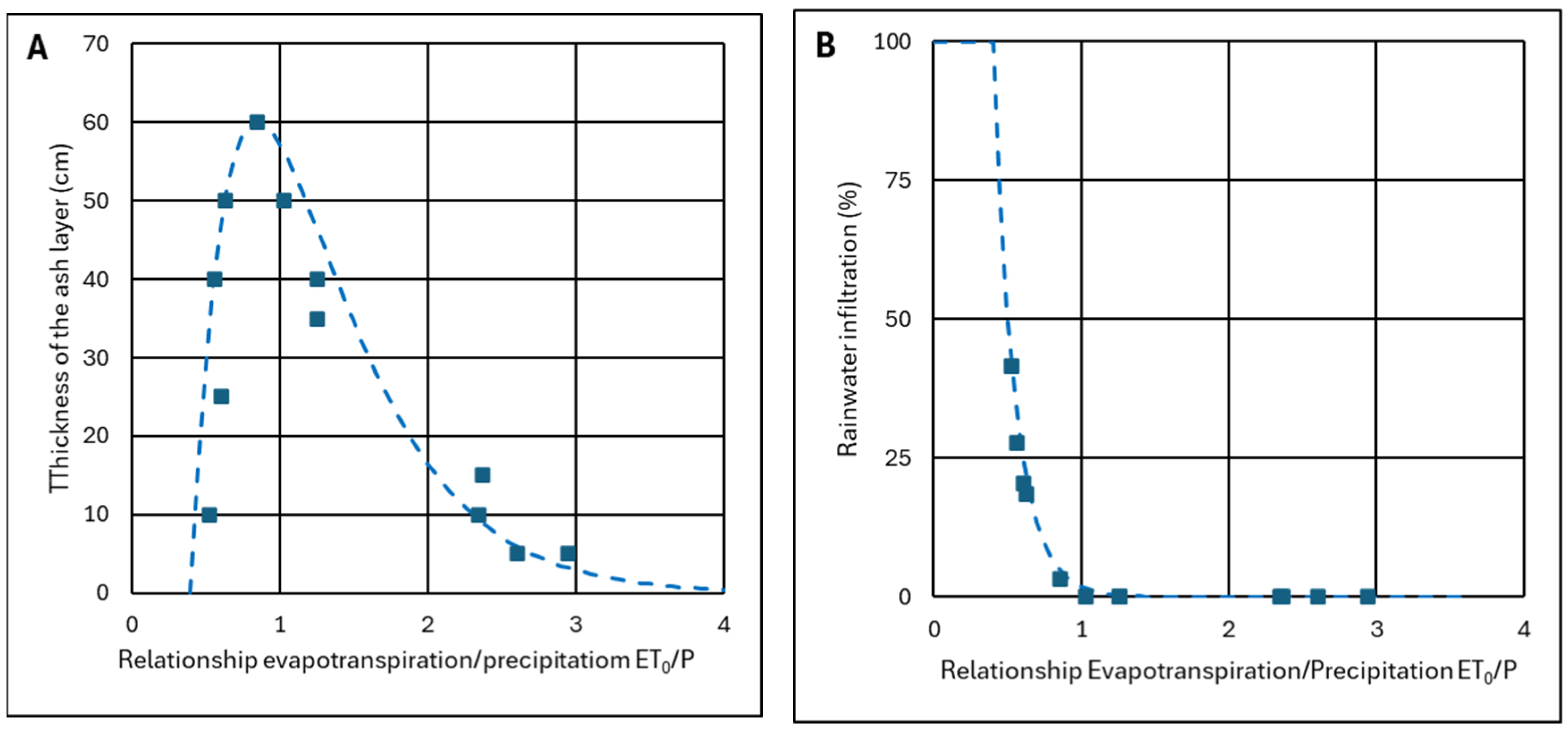
• For ET₀/P ≥ 1, ash can be used as a barrier layer, achieving zero infiltration or waterproofing if the ash layer is thick enough; for values of ET₀/P ≈ 1, thicknesses of h = 50–60 cm will be necessary, which are drastically reduced to h = 10–15 cm when ET₀/P ≥ 2. This ensures that water will not pass through the ash layer because it has sufficient maximum recharge to absorb excess water during rainy seasons. Theoretically, the ash layer could replace a layer of clay or a layer of clay plus a HDPE sheet.
• For ET₀/P < 1, the ash layer can no longer be considered impermeable. With values of ET₀/P ≈ 0.7, a layer of 40–50 cm can be used to stop more than 80% of rainwater. However, a HDPE waterproofing sheet may be required. With ET₀/P ≈ 0.5 values, the worst conditions, it does not make sense for the ash layer to be very thick because it becomes totally saturated and does not have time to dry; however, the ash layer can still be useful since a thickness of only 10–15 cm allows less than 50% of the rainwater to pass through.

The first curve can be represented by a Weibull function:

$$h_u=h_{umax} {\displaystyle \frac{X-X_{min}}{X^{\prime }-X_{min}}} exp\left[1-\left({\displaystyle \frac{X-X_{min}}{X^{\prime }-X_{min}}}\right)\right]$$

(2)

where h_u is the ash layer thickness for minimum infiltration and X = ET₀/P.

X_min = (ET₀/P)_min is the value and the value for the h_u is null; for X < X_min, the ash is not useful and it should not be used. X′ = (ET₀/P)’ is the abscise of the maximum useful thickness h_umax. In our case X_min = 0.4, X′ = 0.85, and h_umax = 60 cm.

On the other hand, the second curve is a negative exponential function:

$$I=I_{max} exp\left[-ln\left({\displaystyle \frac{I^{\prime }}{I_{max}}}\right) {\displaystyle \frac{X-X_{min}}{X^{\prime }-X_{min}}}\right]$$

(3)

where I (%) is the minimum infiltration when h_u is used and X, X′, and X_min have the same meaning. I_max is the maximum infiltration for X = X_min and I′ is the infiltration for X = X′. The maximum possible infiltration is I_max = 100%, and, empirically, we see that a low enough value for the infiltration for X′ = 0.85 is I′ = 5%.

Although the efficiency is lower for low ET₀/P, it is only in relative terms; the volume of water that does not have to be treated is bigger in wet climates. In the studied areas, P and ET₀/P are not completely independent and there is a relationship (Figure 25A):

$$P=P_{min}+\left(P_{max}-P_{min}\right) \mathrm{e}\mathrm{x}\mathrm{p}\left[-k \left(X-X_{min}\right)\right]$$

(4)

where P_max is the maximum yearly precipitation in mm/year; P_min is the minimum yearly precipitation in mm/year and k is an empirical coefficient. According to the data, X_min = 0.4, P_max = 1400 mm/year, P_min = 400 mm/year, and k = 1.5.

The volume of rainwater that is not contaminated, in m³ per m² of covering and year, will be as follows:

$$V={\displaystyle \frac{P}{1000}} \left(1-{\displaystyle \frac{I}{100}}\right)$$

(5)

By substituting Equations (3) and (4) in (5), a new curve can be drawn (Figure 25B). It is evident now that in absolute terms, it is better to avoid the contamination of rainwater in wet regions than in arid ones (70% of 1200 mm/year is bigger than 100% of 500 mm/year).

5. Discussion and Conclusions

Capping contaminated waste to diminish the quantity of leachate produced is a technique with the following advantages:

• The effect is permanent over time as it is based on a physical barrier effect.
• The contamination reduction is independent of the initial concentration.
• The contamination reduction is for any PTE (Hg, Pb, Zn, etc.).

These advantages should inspire a paradigm shift because, in many cases, this could be a solution to help remediate contaminated areas. The standards accepted up to now sought to eliminate the possibility of water infiltration by using totally impermeable barrier elements, either HDPE sheeting and/or clay layers, basing this impermeability on hydraulic conductivities as low as 10⁻¹¹ m/s. However, this requires the use of materials with a significant carbon footprint (the sheet and/or clay) or the exploitation of a valuable natural resource (clay that meets the standards) with the corresponding environmental impact. On the other hand, the materials are expensive, and, because of the extent of the dumps, the economic cost is a major deterrent to undertaking this type of project. Thus, the new paradigm can be summarized in the following points:

• Not trying to achieve absolute waterproofing based only on a very low hydraulic conductivity.
• Using by-products such as fly ash, with sufficiently low hydraulic conductivity and sufficiently high porosity, with sufficient recharge capacity to facilitate evapotranspiration and reduce water infiltration as far as possible.
• Prevent the rainwater from being contaminated is always a good result and, even if 100% waterproofing is not achieved, it can be a successful result in many cases.
• Reducing the volume of contaminated water results in economic savings because treatments for eliminating PTEs of the contaminated water are usually expensive.
• The leachate contamination reduction, due to the dilution in the water of the rivers, greatly reduces the extent of contamination so that the maximum concentration levels are closer to the source of contamination.

The proposed solution is complementary to the existing ones and can be very useful in cases such as leachates with concentrations slightly higher than the legal limits. In this sense, it is necessary to look for an ash thickness that complies with the following:

• The recharge is sufficiently large to absorb the maximum difference between precipitation and evapotranspiration.
• Infiltration is theoretically null or as little as possible.
• The recharge balances evapotranspiration in the dry season, ensuring that the planted species always have moisture.

Given the permeability and porosity characteristics of the ashes and the balanced relationship ET₀/P, in the case study from the north of Spain, this is achieved with a thickness of the ash layer of about 45 cm, which provides a recharge of about 250 mm.

References

1. Giusti, L. A Review of Waste Management Practices and Their Impact on Human Health. Waste Manag. 2009, 29, 2227–2239. [Google Scholar] [CrossRef] [PubMed]
2. Asokan, P.; Saxena, M.; Asolekar, S.R. Coal Combustion Residues—Environmental Implications and Recycling Potentials. Resour. Conserv. Recycl. 2005, 43, 239–262. [Google Scholar] [CrossRef]
3. Babbitt, C.W.; Lindner, A.S. A life cycle comparison of disposal and beneficial use of coal combustion products in Florida. Part 1: Methodology and input and emissions inventory. Int. J. Life Cycle Assess. 2008, 13, 555–563. [Google Scholar] [CrossRef]
4. Demir, I.; Hughes, R.E.; DeMaris, P.J. Formation and Use of Coal Combustion Residues from Three Types of Power Plants Burning Illinois Coals. Fuel 2001, 80, 1659–1673. [Google Scholar] [CrossRef]
5. Rodella, N.; Pasquali, M.; Zacco, A.; Bilo, F.; Borgese, L.; Bontempi, N.; Tomasoni, G.; Depero, L.E.; Bontempi, E. Beyond waste: New sustainable fillers from fly ashes stabilization, obtained by low cost raw materials. Heliyon 2016, 2, e00163. [Google Scholar] [CrossRef]
6. Adamczyk, Z.; Komorek, J.; Białecka, B.; Nowak, J.; Klupa, A. Assessment of the potential of polish fly ashes as a source of rare earth elements. Ore Geol. Rev. 2020, 124, 103638. [Google Scholar] [CrossRef]
7. Ahmaruzzaman, M. A review on the utilization of fly ash. Prog. Energy Combust. Sci. 2010, 36, 327–363. [Google Scholar] [CrossRef]
8. Babbitt, C.W.; Lindner, A.S. A Life Cycle Inventory of Coal Used for Electricity Production in Florida. J. Clean. Prod. 2005, 13, 903–912. [Google Scholar] [CrossRef]
9. Woodward-Clyde Consultants Report on Combustion By-Products in Florida; Provided courtesy of the Florida Electric Utility Coordinating Group: Tallahassee, FL, USA, 1994.
10. Zhao, Y.P.; Zhao, L.; Feng, L.; Yang, Y. Hazardous Contaminants in the Environment and Their Laccase-Assisted Degradation—A Review. J. Environ. Manag. 2019, 234, 253–264. [Google Scholar] [CrossRef]
11. Malhotra, V.M. Durability of concrete incorporating high-volume of lowcalcium (ASTM Class F) fly ash. Cem. Concr. Compos. 1990, 12, 271–277. [Google Scholar] [CrossRef]
12. Pereira, C.F.; Luna, Y.; Querol, X.; Antenucci, D.; Vale, J. Waste stabilization/solidification of an electric arc furnace dust using fly ash-based geopolymers. Fuel 2009, 88, 1185–1193. [Google Scholar] [CrossRef]
13. Sobolev, K.; Vivian, I.F.; Saha, R.; Wasiuddin, N.M.; Saltibus, N.E. The effect of fly ash on the rheological properties of bituminous materials. Fuel 2014, 116, 471–477. [Google Scholar] [CrossRef]
14. Teixeira, E.R.; Mateus, R.; Cames, A.F.; Bragana, L.; Branco, F.G. Comparative environmental life-cycle analysis of concretes using biomass and coal fly ashes as partial cement replacement material. J. Clean. Prod. 2016, 112, 2221–2230. [Google Scholar] [CrossRef]
15. Embong, R.; Kusbiantoro, A.; Shafiq, N.; Nuruddin, M.F. Strength and microstructural properties of fly ash based geopolymer concrete containing highcalcium and water-absorptive aggregate. J. Clean. Prod. 2016, 112, 816–822. [Google Scholar] [CrossRef]
16. Hu, G.; Liu, H.; Chen, C.; Li, J.; Hou, H.; Hewage, K.; Sadiq, R. An integrated geospatial correlation analysis and human health risk assessment approach for investigating abandoned industrial sites. J. Environ. Manag. 2021, 293, 112891. [Google Scholar] [CrossRef]
17. Mhlongo, S.E. Physical hazards of abandoned mines: A review of cases from South Africa. Extr. Ind. Soc. 2023, 15, 101285. [Google Scholar] [CrossRef]
18. Méndez-Fernández, L.; Rodríguez, P.; Martínez-Madrid, M. Sediment Toxicity and Bioaccumulation Assessment in Abandoned Copper and Mercury Mining Areas of the Nalón River Basin (Spain). Arch. Environ. Contam. Toxicol. 2015, 68, 107–123. [Google Scholar] [CrossRef]
19. Teunen, L.; Belpaire, C.; De Boeck, G.; Blust, R.; Bervoets, L. Mercury Accumulation in Muscle and Liver Tissue and Human Health Risk Assessment of Two Resident Freshwater Fish Species in Flanders (Belgium): A Multilocation Approach. Environ. Sci. Pollut. Res. 2022, 29, 7853–7865. [Google Scholar] [CrossRef]
20. Castilhos, Z.C.; Rodrigues-Filho, S.; Rodrigues, A.P.; Villas-Bôas, R.C.; Siegel, S.; Veiga, M.M.; Beinhoff, C. Mercury Contamination in Fish from Gold Mining Areas in Indonesia and Human Health Risk Assessment. Sci. Total Environ. 2006, 368, 320–325. [Google Scholar] [CrossRef]
21. He, F.; Gao, J.; Pierce, E.; Strong, P.J.; Wang, H.; Liang, L. In Situ Remediation Technologies for Mercury-Contaminated Soil. Environ. Sci. Pollut. Res. 2015, 22, 8124–8147. [Google Scholar] [CrossRef]
22. Hylander, L.D.; Meili, M. 500 Years of Mercury Production: Global Annual Inventory by Region until 2000 and Associated Emissions. Sci. Total Environ. 2003, 304, 13–27. [Google Scholar] [CrossRef] [PubMed]
23. Lin, Y.; Larssen, T.; Vogt, R.D.; Feng, X. Identification of Fractions of Mercury in Water, Soil and Sediment from a Typical Hg Mining Area in Wanshan, Guizhou Province, China. Appl. Geochem. 2010, 25, 60–68. [Google Scholar] [CrossRef]
24. Ordóñez, A.; Álvarez, R.; Charlesworth, S.; Miguel, E.D.; Loredo, J. Risk Assessment of Soils Contaminated by Mercury Mining, Northern Spain. J. Environ. Monit. 2011, 13, 128–136. [Google Scholar] [CrossRef] [PubMed]
25. Sánchez-Castro, I.; Molina, L.; Prieto-Fernández, M.A.; Segura, A. Past, present and future trends in the remediation of heavy metal contaminated soil—Remediation techniques applied in real soil-contamination events. Heliyon 2023, 9, 16692. [Google Scholar] [CrossRef]
26. Wang, L.; Hou, D.; Cao, Y.; Ok, Y.S.; Tack, F.M.G.; Rinklebe, J.; O’Connor, D. Remediation of Mercury Contaminated Soil, Water, and Air: A Review of Emerging Materials and Innovative Technologies. Environ. Int. 2020, 134, 105281. [Google Scholar] [CrossRef]
27. Parameswaran, K. Sustainability considerations in innovative process development. In Innovative Process Development in Metallurgical Industry; Springer: Berlin/Heidelberg, Germany, 2016; pp. 257–280. [Google Scholar]
28. Santibánez, C.; Verdugo, C.; Ginocchio, R. Phytostabilization of copper mine tailings with biosolids: Implications for metal uptake and productivity of Lolium perenne. Sci. Total Environ. 2008, 395, 1–10. [Google Scholar] [CrossRef]
29. Rodríguez, R.; Hernández, Z.; Fernández, B.; Bascompta, M. A Novel Solution to Avoid Mercury Emissions Produced by Highly Contaminated Demolition Debris in Mining Site. Environments 2023, 10, 187. [Google Scholar] [CrossRef]
30. Chazarra, A.; Flórez, E.; Peraza, B.; Tohá, T.; Lorenzo, B.; Criado, E.; Moreno, J.V.; Romero, R.; Bote, R. Mapas Climáticos de España (1981–2010) y ETo (1996–2016); Ministerio para la Transición Ecológica, Agencia Estatal de Meteorología: Madrid, Spain, 2018; p. 75. [Google Scholar]
31. Sancho, J.M.; Riesgo, J.; Jiménez, C.; Sánchez, M.C.; Montero, J.; López, M. Atlas de Radiación Solar en España Utilizando Datos del SAF de Clima de EUMETSAT; Agencia Estatal de Meteorología (AEMET): Madrid, Spain, 2012; p. 162. [Google Scholar]
32. Ayala, J.; Fernández, B. Industrial waste materials as adsorbents for the removal of As and other toxic elements from an abandoned mine spoil heap leachate: A case study in Asturias. J. Hazard. Mater. 2020, 384, 121446. [Google Scholar] [CrossRef]
33. European Standards UNE EN 12457-4:2003; Characterisation of Waste: Leaching: Compliance Test for Leaching of Granular Waste Materials and Sludges—Part 4: One Stage Batch Test at a Liquid to Solid Ratio of 10 L/kg for Materials with Particle Size Below 10 mm (without or with Size Reduction). Asociación Española de Normalización: Madrid, Spain, 2003.
34. Vaselli, O.; Nisi, B.; Rappuoli, D.; Cabassi, J.; Tassi, F. Gaseous Elemental Mercury and Total and Leached Mercury in Building Materials from the Former Hg-Mining Area of Abbadia San Salvatore (Central Italy). Int. J. Environ. Res. Public Health 2017, 14, 425. [Google Scholar] [CrossRef]
35. European Standards UNE-EN 1097-3:1999; Tests for Mechanical and Physical Properties of Aggregates—Part 3: Determination of Loose Bulk Density and Voids. Asociación Española de Normalización: Madrid, Spain, 1999.
36. European Standards UNE-EN 1097-6:2014; Tests for Mechanical and Physical Properties of Aggregates—Part 6: Determination of Particle Density and Water Absorption. Asociación Española de Normalización: Madrid, Spain, 2014.
37. European Standards UNE-EN 450-1:2013; Fly Ash for Concrete—Part 1: Definition, Specifications and Conformity Criteria. Asociación Española de Normalización: Madrid, Spain, 2013.
38. European Standards UNE-EN ISO 17892-11:2020; Geotechnical Investigation and Testing - Laboratory Testing of Soil—Part 11: Permeability Tests (ISO 17892-11:2019). Asociación Española de Normalización: Madrid, Spain, 2020.
39. CEDEX; Centro de Experimentación y Estudios de Obras Públicas. Ficha Técnica: Cenizas Volantes de Carbón y Cenizas de Hogar o Escorias; Ministerio de Fomento y Ministerio de Medio Ambiente: Madrid, Spain, 2011. [Google Scholar]
40. García-Fraile, J. Caracterización de Cenizas de Centrales Térmicas del Norte de España para su Aplicación en Usos Alternativos. Master’s Thesis, Universidad de Oviedo, Oviedo, Spain, 2015. [Google Scholar]
41. Yu, Z.; Lue, H.; Zhu, Y.; Drake, S.; Liang, C. Long-term effects of revegetation on soil hydrological processes in vegetation-stabilized desert ecosystems. Hydrol. Process 2010, 24, 87–95. [Google Scholar] [CrossRef]
42. Jiao, J.Y.; Zhang, Y.; Zhu, J.T. Direct hydraulic parameter and function estimation for diverse soil types under infiltration and evaporation. Transp. Porous Media 2017, 116, 797–823. [Google Scholar] [CrossRef]
43. Niu, W.Q.; Zou, X.Y.; Liu, J.J.; Zhang, M.Z.; Lü, W.; Gu, J. Effects of residual plastic film mixed in soil on water infiltration, evaporation and its uncertainty analysis. Trans. Chin. Soc. Agric. Eng. 2016, 32, 110–119. [Google Scholar] [CrossRef]
44. Wang, Z.C.; Li, X.Y.; Shi, H.B.; Zhang, D.L.; Xu, P.C. Effects of residual plastic film on infiltration and evaporation for sandy loam and sandy soil. Trans. Chin. Soc. Agric. Eng. 2017, 48, 198–205. [Google Scholar] [CrossRef]
45. Fan, C.; Guo, J.; Li, X.; Zhang, C.; Wang, T. Effects of enclosure measures on soil water infiltration and evaporation in arid and semi-arid grassland in northern China. Front. Environ. Sci. 2024, 12, 1410037. [Google Scholar] [CrossRef]
46. Ghiat, I.; Mackey, H.R.; Al-Ansari, T. A Review of Evapotranspiration Measurement Models, Techniques and Methods for Open and Closed Agricultural Field Applications. Water 2021, 13, 2523. [Google Scholar] [CrossRef]
47. Allen, R.G.; Pereira, L.S.; Raes, D.; Smith, M. Crop Evapotranspiration: Guidelines for Computing Crop Water Requirements—FAO Irrigation and Drainage; Food and Agriculture Organization of the United Nations, FAO: Rome, Italy, 1998; Available online: https://www.fao.org/4/x0490e/x0490e00.htm (accessed on 15 July 2024).
48. Neukum, C.; Morales-Santos, A.; Ronelngar, M.; Bala, A.; Vassolo, S. Modelling groundwater recharge, actual evaporation, and transpiration in semi-arid sites of the Lake Chad basin: The role of soil and vegetation in groundwater recharge Hydrol. Earth Syst. Sci. 2023, 27, 3601–3619. [Google Scholar] [CrossRef]
49. Thornthwaite, C.W. An approach toward a rational classification of climate. Geogr. Rev. 1948, 38, 55–94. [Google Scholar] [CrossRef]
50. Turc, L. Estimation of irrigation water requirements, potential evapotranspiration: A simple climatic formula evolved up to date. Ann. Agron. 1961, 12, 13–49. [Google Scholar]
51. Hargreaves, G.H.; Samani, Z.A. Reference crop evapotranspiration from temperature. Appl. Eng. Agric. 1985, 1, 96–99. [Google Scholar] [CrossRef]
52. Coly, O.; Weihermüller, L.; Ba, K.; Faye, S.C.; Faye, S.; Vereckeen, H. Estimation of Turc reference evapotranspiration with limited data against the Penman-Monteith Formula in Senegal. J. Agric. Environ. Int. Dev. 2016, 110, 117–137. [Google Scholar] [CrossRef]
53. Bernard, M.M. Formulas for rainfall intensities of long durations. Trans. ASCE 1932, 96, 592–624. [Google Scholar]
54. Chow, V.T. Hydrologic Determination of Waterway Areas for Drainage Structures in Small Drainage Basins; Bulletin No. 462, Engineering. Experimental Station; University of Illinois Urbana-Champaign: Champaign, IL, USA, 1962. [Google Scholar]
55. Pizarro, R.; Abarza, A.; Farías, C.; Jordán, C. Construcción de Curvas IDF (Intensidad-Duración-Frecuencia) en zonas semiáridas de Chile Central. In Proceedings of the Actas del XII Congreso Forestal Mundial, Quebec, QC, Canada, 21–28 September 2003. [Google Scholar]
56. Moncho, R.; Belda, F.; Caselles, V. Climatic study of the exponent n of the IDF curves of the Iberian Peninsula. J. Weather Clim. West. Mediterr. 2009, 6, 3–14. [Google Scholar] [CrossRef]
Figure 1. Facilities in early 1970s and demolished structures with in situ debris in 2017.
Environments 12 00107 g001
Figure 2. Average annual precipitation in Spain and Asturias modified from Chazarra et al. [30].
Environments 12 00107 g002
Figure 3. Average annual evapotranspiration in Spain and Asturias, modified from Sancho et al. [31].
Environments 12 00107 g003
Figure 4. Different types of waste and debris of metallurgical plant demolition in the study area.
Environments 12 00107 g004
Figure 5. Location of the 11 solid sampling points (red) and leachate sampling points (blue).
Environments 12 00107 g005
Figure 6. Water penetrating before saturation (A) and water infiltration after saturation (B).
Environments 12 00107 g006
Figure 7. Covering demolition debris (A) and location of sampling points in the ash capping (B).
Environments 12 00107 g007
Figure 8. Monitoring rainwater, temperature, and ultraviolet radiation.
Environments 12 00107 g008
Figure 9. Ash sampling for ash wetness determination.
Environments 12 00107 g009
Figure 10. Test tubes with ashes to determine the infiltration.
Environments 12 00107 g010
Figure 11. Precipitation (A) and water recharge in the ash (B) during the 3 monitoring months.
Environments 12 00107 g011
Figure 12. Maximum recharge before saturation (A) and water infiltration after ash saturation (B).
Environments 12 00107 g012
Figure 13. Precipitation during the water year.
Environments 12 00107 g013
Figure 14. Variation in water recharge in the ashes during the water year.
Environments 12 00107 g014
Figure 15. Variation in water recharge with ash thicknesses of 30 cm (A) and 60 cm (B).
Environments 12 00107 g015
Figure 16. Relationship between layer thickness–infiltration (A) and evapotranspiration–precipitation (B).
Environments 12 00107 g016
Figure 17. Location of the selected mining areas and thermal power plants in Spain.
Environments 12 00107 g017
Figure 18. Climatological data in zone 10: monthly average (A) and cumulative values (B).
Environments 12 00107 g018
Figure 19. Water infiltration (A) and water recharge (B) in zone 10.
Environments 12 00107 g019
Figure 20. Climatological data in zone 6: monthly average (A) and cumulative values (B).
Environments 12 00107 g020
Figure 21. Water infiltration (A) and water recharge (B) in zone 6.
Environments 12 00107 g021
Figure 22. Climatological data in zone 2: monthly average (A) and cumulative values (B).
Environments 12 00107 g022
Figure 23. Water infiltration (A) and water recharge (B) in zone 2.
Environments 12 00107 g023
Figure 24. Estimation of the necessary layer thickness (A) and infiltration (B) based on ET0/P.
Environments 12 00107 g024
Figure 25. Yearly precipitation (A) and contaminated rainwater volume (B) as a function of ET0/P.
Environments 12 00107 g025