Fishponds Are Hotspots of Algal Biodiversity—Organic Carp Farming Reveals Unexpected High Taxa Richness

Abstract

Fishponds are regarded as hypertrophic systems accompanied by low biodiversity. We focused on the phytoplankton diversity of 15 fishponds located in Austria. Of the 15 fishponds, 12 waterbodies are aquaculture ponds stocked with common carp, which converted to organic farming some years ago with grain as supplementary feed, and 3 ponds are used for recreational fishing. The trophic state index increased from 59 to 71 in spring to 80 to 93 in autumn and classified the ponds as mid-eutrophic to hypertrophic. The taxa number was surprisingly high (taxa richness up to 100 taxa per pond). The phytoplankton resource use efficiency was in the upper range of eutrophicated waters and did not show seasonal differences (median Chlorophyll-a/total phosphorus = 1.94, Chlorophyll-a/total nitrogen = 0.12). Linking environmental data with the algal community resulted in a distinct temporal community pattern with a significant seasonal shift from the cooler season dominated by Ochrophyta taxa to green algae as the most abundant group in summer and autumn. Our findings challenge general assumptions regarding low phytoplankton diversity with long-lasting Cyanobacteria blooms and conform to the algal dynamics described in the plankton ecology group (PEG) model for temperate shallow lakes. These man-made systems are an ecological asset, highly connected to terrestrial habitats in their vicinity and significantly contributing to the ecological health and long-term sustainability of the region.

1. Introduction

Pond aquaculture has a long tradition in Austria and neighboring countries [1] with the most stocked fish common carp being Cyprinus carpio L. Although the primary focus of pond aquaculture is on fish yield, the biocoenosis of ponds is tightly interconnected, therefore fish farming must be seen in a broader context. Aside from providing economic benefits—around 500 t of carp are produced annually in the Waldviertel [2]—ponds and their surroundings play a crucial ecological role in providing refuges and breeding habitats to endangered and protected wildlife, including water birds such as black-headed gull (Chroicocephalus ridibundus L.) and black stork (Ciconia nigra L.) [3,4]. Ponds are also interlinked with land ecosystems. One prime example is amphibiotic insects, which transport high-quality metabolic products from the ponds into the terrestrial environment [5,6]. Furthermore, pond management practices such as winter draining of ponds facilitate the formation of short-lived pioneer habitats, which are crucial for maintaining the integrity of wetland ecosystems [7,8].

Pond aquaculture was first documented in Austria during the late 13th century [9]. Due to population growth and food shortages in the late 18th century, aquaculture gradually declined after centuries of development. Following the Second World War, fish farming returned to prominence [7]. Currently, more than 1800 ponds with an overall area of approximately 1700 ha exist in the Waldviertel region, Lower Austria [2]. Commercial fish farming is the primary purpose of most of the ponds in this area, but some ponds are also visited for sport fishing and recreation. Waldviertel ponds are classified as part of Ramsar wetlands in Austria and are included in the “Natura 2000—Europaschutzgebiete Waldviertler Teich-, Heide- and Moorlandschaft und Waldviertel” as well. Most recent research mentioning microalgae taxa in Waldviertel water bodies dates back more than half a century ago, but the studies focused on different ponds, and only part of them have been used for pond farming [10,11,12]. For the nearby Czech Republic, a few recent studies dealing with phytoplankton do exist [13,14,15,16].

Phytoplankton is an indispensable component for the sustainable operation of outdoor fish farming systems [17,18]. It is highly involved in nutrient cycling, oxygen supply during the day, and oxygen consumption during the night. High phytoplankton biomass, which is a common feature of fishponds, may cause critical diurnal oscillations of dissolved oxygen, which are detrimental to the whole pond community [19]. Microalgae provide proteins and carotenoids and are also one primary source for polyunsaturated fatty acids (PUFAs) [20,21]. In the trophic cascade, they are either directly consumed by phytoplanktivorous fish [22] or indirectly via zooplankton and -benthos [23,24]. Strangely, studies focusing on the phytoplankton community are largely neglected in pond farming research compared to other components of the food web. Since the transition of fishponds in Waldviertel into organic farming, microalgae communities have not been studied.

Fishponds are characterized by high nutrient load due to fish feed as well as inputs from the atmosphere, adjacent agriculture, and catchment areas, which result in eutrophic to hypertrophic conditions [25,26]. In addition, benthivorous fish like carp cause sediment resuspension, resulting in an increase in turbidity and phosphorus content in the water column [27,28,29,30]. Moreover, especially given a shortage of essential amino acids lysine and methionine, carps might excrete soluble reactive phosphorus (SRP) into the environment [31]. Excessive nitrogen levels may also occur as a result of fish excretion, feeding on natural food [32,33], and the degradation of organic matter, including leftover fish feed and dead organisms [34,35]. Consequently, this surplus of nutrients and an increase in turbidity lead to eutrophication, often recognized as long-lasting blooms of Cyanobacteria of low diversity [14,16,36]. Cyanobacteria blooms are not restricted to fishponds, they occur in both inland waters and the sea and have become more frequent globally due to eutrophication, rising atmospheric CO₂ levels, and global warming [37,38,39]. Eutrophicated shallow lakes—fishponds have some comparable features—are prone to such blooms as they offer environmental conditions favored by cyanobacteria [40,41,42]. Increased turbidity promotes the development of certain Cyanobacteria taxa due to their ability to rise to the surface of the water column with the aid of gas vesicles [43]. Moreover, an increase in fish farming intensity may induce a transition from large colonial forms to filaments or single-celled forms [44]. For such patterns, a low N/P ratio is a possible explanation because it has negative effects on the buoyancy of colonial Cyanobacteria such as Microcystis [45]. The drop in N/P may be caused by denitrification, which is pronounced in shallow lakes [46] and further boosted by turbulences at the water–sediment interface [47].

Certain Cyanobacteria are a serious problem and may cause massive fish mortality [36,48,49]. This group is of minor quality as a feed for zooplankton and is often inedible [42,50]. Most cyanobacterial taxa found in eu- to hypertrophic water bodies are colonial and filamentous pelagic forms, which may clog the filtering apparatus of zooplankton, which is an important component of fish diets [51,52,53,54]. In addition, certain Cyanobacteria taxa synthesize toxic substances. Exposure to cyanotoxins can result in decreased survival and growth rates of fish [55,56,57]. Moreover, accumulating in fish tissues, these substances pose a health hazard to fish as well as to humans through consumption [55,58]. Some Cyanobacteria synthesize geosmin, which contributes to the sometimes muddy–earthy taste of common carp [59]. Due to its ability to accumulate in fish flesh through dietary and environmental exposure, it can have a detrimental impact on consumer acceptance and lead to financial losses for fish farmers [60]. In particular, common genera such as Oscillatoria, Dolichospermum, and Nostoc have been identified as producers of geosmin [61,62].

For Czech fishponds, it was demonstrated that excessive fish feeding impairs both water and sediment quality: mass development of phytoplankton, accompanied by great fluctuations in oxygen content and pH, are a threat to most organisms inhabiting the ponds [42,63]. High respiration and decomposition processes may moreover lead to anoxic conditions in bottom-near zones [19] (especially during night), thus promoting internal phosphorus loading, perpetuating a feedback loop [64,65]. Pronounced pH fluctuations mainly occur in bedrocks with low buffer capacity, such as silicate bedrock found in the region. This is of special importance, as changes in pH also cause a shift of pH-dependent chemical equilibria such as ammonium to toxic ammonia [66]. High nutrient load has also a negative impact on the trophic structure of fishponds with a decoupling of microbial food web components and herbivorous crustaceans [67]. All these challenges are mostly related to conventional fish farming, high density fish stock, and overfeeding of fish coupled with improper diet composition. The way out is organic farming with both balanced fish diets [32] and demand-oriented feeding [54,68]. Worldwide, only around 0.5% of aquacultures are operated on organic guidelines [69]; in Austria, approximately 20% have been converted to organic farming [7]. In these systems, added organic fish feed is combined with available natural food sources, which reduces nutrient load [54].

With the current study, we intend to add detailed environmental and biological data for fishponds, which have been converted to organic farming. The data provide new insights into species distribution and community patterns. Gained information will be beneficial for future pond management and the local community, who rely on fishponds as a source of income and recreational activities. We explored phytoplankton biodiversity along environmental gradients in a set of fishponds. Overall, 3 ponds are mainly visited for recreational activities, and 12 more waterbodies are used for pond farming. We compared these two groups for differences in the community structure and expected significant differences in their community composition. We focused on three seasons, spring, summer, and fall, during which the stocked ponds are run, and assumed that algae composition will vary between seasons and between sites due to differences in both biotic and abiotic factors. Diversity was anticipated to be generally low in fishponds because of eutrophication, which should also be reflected in low phytoplankton resource use efficiency (RUE) [70]. RUE is interpreted as a measure to compare the actual productivity with the potential one. Low biodiversity is assumed to be less efficient in use of available resources [71], which will be reflected in low RUE. We expected the dominance of colonial and filamentous Cyanobacteria during summer, with some of them developing gas vesicles, which facilitate buoyancy, because this group is promoted by elevated water temperature and pH, increased nutrient load, and higher fish activity, contributing to high turbidity.

2. Material and Methods

2.1. Study Site Description

The Waldviertel plateau, covering an area of around 4.615 km² and ranging from 400 m to 900 m above sea level [4], is located in the southern part of the Bohemian Massif, which constitutes one of the mid-range mountains of Europe. The bedrock is granite and gneiss [72], which affects the hydrochemistry of the ponds. The climate is continental, with the mean annual air temperature ranging between 4 and 7 °C. The precipitation reduces from the forested west, with an average yearly rainfall of about 800 mm to 500 mm toward the drier east [73]. Most fishponds are so-called “sky ponds”, mainly fed by rainwater runoff from neighboring fields. Details are available from Bundesministerium für Land- und Forstwirtschaft [74].

We studied 15 fishponds located in three municipal districts Heidenreichstein (1 Steinbruckteich, 2 Winkelauer Teich, 3 Edelwehrteich, 4 Streitteich, 5 Neuteich, 6 Brüneiteich, 7 Brandteich), Schrems (8 Haslauer Teich, 9 Gebhartsteich, 10 Moorbad, 11 Höfentöckteich), and Pürbach (12 Pürbacher Teich, 13 Althöllteich, 14 Frauenteich, 15 Edlauerteich; number are used in the following sections). Sizes vary greatly between 2.7 and 57.0 ha, and maximum depths are between 2.5 and 3.5 m. Most of the ponds are currently managed for 1 to 2 years, except for the ponds used for sport fishing and swimming (3, 10, 11), which have been in permanent operation for an estimated 20 years. For the managed ponds, water drains through the monk, which pools the fish toward a small area called the fish dump. Immediately after fish harvest, refilling starts again, which takes several weeks. Neither are the ponds dried out completely nor are they cleaned. Fish harvest ranges from 260 to 700 kg ha⁻¹, with carp being the main fish in all ponds but with other species occurring (e.g., vendace and white fish). In 2021, supplemental grain feeding was carried out in the 12 managed ponds (because of trade secret, no detailed data are available). Liming is performed in certain ponds in the area of the fish dump while wind turbines are utilized only in pond 11 for surface ventilation to avoid oxygen deficits. For more details on the individual fishponds, refer to

Table 1. General information of investigated ponds. (HD: Heidenreichstein, SCH: Schrems, PÜR: Pürbach, H: Sky pond, S: Stream pond, C: Carp farming, F: Fishing, B: Bathing).

Labelling	District	Pond	Area (ha)	Age (y)	Sea Level (m)	Type	Stocking Amount (Indivudual ha−1)	Usage	Liming	GPS
1	HD	Steinbruckteich	8.73	250	605	H	3000	C	No	48.8591, 15.1464
2	HD	Winkelauerteich	49.27	250	597	H/S	650	C	Yes	48.8455, 15.1457
3	HD	Edelwehrteich	3.13	210	561	S		F	No	48.8728, 15.1333
4	HD	Streitteich	2.76	250	574	H	3000	C	No	48.8792, 15.1270
5	HD	Neuteich	4.36	250	564	H	3000	C	No	48.8713, 15.1235
6	HD	Gr. Brünaiteich	30.00	250	550	H	550	C	Yes	48.8720, 15.0647
7	HD	Brandteich	15.22	250	524	H	3000	C	Yes	48.8592, 15.0308
8	SCH	Haslauerteich	50.00	50	560	S	650	C	No	48.8230, 15.1331
9	SCH	Gebhartsteich	57.00	250	547	S	650	C	Yes	48.80214, 15.1385
10	SCH	Moorbad	3.00	250	532	H		F/B	Yes	48.8000, 15.0793
11	SCH	Höfentöckteich	15.00	250	517	H		F	Yes	48.7893, 15.0380
12	PÜR	Pürbacher Teich	21.20	250	526	H/S	650	C	No	48.7704, 15.0752
13	PÜR	Althöllteich	19.00	250	572	H/S	650	C	No	48.7660, 15.0724
14	PÜR	Frauenteich	26.58	250	536	H/S	650	C	No	48.7540, 15.0875
15	PÜR	Edlauteich	20.96	250	534	H/S	650	C	No	48.7542, 15.0691

.

2.2. Field Sampling and In Situ Measurements

Sampling was conducted in 3 seasons on 7 April, 6 July, and 16 September of 2021. Phytoplankton and water samples were collected at the deepest part of the pond called monk, through which the pond water can be drained (maximum depths of the investigated ponds were between 2.5 and 3.5 m). A plankton net with a mesh size of 30 µm was used to collect larger forms. After being transferred into Greiner tubes, part of the sample was fixed with one drop of paraformaldehyde. In parallel, raw water samples for membrane filtration of small plankton forms and hydrochemistry were taken using a Schindler sampler from the uppermost 0.5 m and near the bottom, they were mixed in canisters for depth-integrated samples and transported to the laboratory in an ice box at 4 °C for further analysis. For quantitative Zooplankton sampling, a Schindler sampler was used to collect 20 L water from the surface and near the bottom (integrated sample). The water was then filtered through a 100 µm sieve, and the concentrated zooplankton were transferred into flasks and fixed with ethanol for preservation.

Temperature, pH value, dissolved oxygen, and conductivity were measured on site with portable meters (multiparametric analyzer WTW Multi 3630 IDS Xylem, Washington, DC, USA) equipped with sensors FDO^® 925 for dissolved oxygen and temperature, TetraCon^® 925 for conductivity, and SensoLyt 900^® for pH). Water transparency was estimated via Secchi-disc readings. The total alkalinity was determined on site using acidimetric titration of the raw water (MQuant Kompaktlabor Test kit, Merck KGaA, Darmstadt, Germany).

2.3. Dry Mass, Ash Mass, and Pigments

To determine the dry mass (DM), a defined volume of pond water was filtered using pre-combusted and pre-weighed glass fiber filters with vacuum filtration (Whatman GF/C; particle retention: 1.2 µm). Filters were then dried in a drying cabinet at 90 °C for a minimum of 24 h. Subsequently, the filters were reweighed, and the DM was calculated using the following formula: DM (mgL⁻¹) = ((Filter incl. material (mg)-empty filter (mg))/)/(filtered volume (L)) ⁻¹. DM filters were then combusted at 500 °C for 2 h in a muffle furnace. To determine the ash mass (AM), the filters were reweighed after cooling. Ash-free dry mass (AFDM or POM, the organic component of the sample) was calculated by subtracting AM from DM.

For photosynthetic pigments analysis, a defined volume of the raw water sample was filtered on a glass fiber filter (Whatman GF/C; particle retention: 1.2 µm, Cytiva, Marlborough, MA, USA), which then became wrapped up in aluminum foil and stored at −20 °C until further processing. The frozen filters were subsequently cut and homogenized using ultrasonication (Branson Sonifier 250, Danbury, CT, USA) after being resuspended in 6 mL of 90% acetone. The extraction process was carried out in the dark at 4 °C for 12 h. The extract was then centrifuged, and the resulting supernatant was analyzed using a spectrophotometer (Hitachi U-2000, Tokyo, Japan) at a wavelength of 663 nm. Calculation of chlorophyll-a (Chl-a) was performed as follows [75]: Chl-a (µgL⁻¹) = (11.40 × E663 × v(mL))/(V(L) × d(cm)) with E663 = absorbance at 663 nm; v = volume of the extract; V = sample volume; d = cuvette path length. In addition, the extract was also analyzed by means of high-performance liquid chromatography (HPLC) with peak detection at 440 nm (Merck-Hitachi LaChrom Elite HPLC System, Tokyo, Japan, equipped with a L-2455 diode array detector and L-2485 FL-detector, gradient program Van Heukelem and Thomas [76]) for delimiting algal groups by their specific pigments [77]. For the group separation of Cyanoprokaryotes, Dino- and Euglenophyta, Bacillario- and Chrysophyceae, and green algae, chlorophyll c, peridin, fucoxanthin, neoxanthin, violaxanthin, diadinoxanthin, lutein, chlorophyll-b, and echinenone based on Chl-a were taken. A mixed standard containing 28 pigments (DHI Lab Products, Hørsholm, Denmark) was used for peak identification. Group contributions were calculated with the routine CHEMTAX 1.9.5 [78].

2.4. Water Chemistry

Cations (OENORM DIN EN ISO 14911) and anions (DIN EN ISO 10304-1) were analyzed using a Metrohm 761 Compact ion chromatography (Cation column: Metrohm Metrosep C2; Anion column: Metrohm Metrosep A Supp 5) of filtrated samples (0.45 μm filters, Whatman Puradisc, UK). The total phosphorus (TP) was evaluated after wet combustion of unfiltered samples (OENORM DIN EN ISO 6878) using a spectrophotometer at 890 nm (Hach-Lange DR 2800). The contents of soluble reactive phosphorus (SRP), nitrite-N (NO₂-N), ammonium-N (NH₄-N), and silicate (SiO₄-Si) were measured in filtrates obtained by filtering the samples through 0.45 μm filters (Whatman Puradisc, UK) using photometric methods: SRP with α-phosphomolybdenum blue at 890 nm (OENORM DIN EN ISO 6878) and NO₂-N via diazotization as a violet-red azo dye at 542 nm (DIN EN ISO 26777). NH₄-N was determined photometrically using the indophenol-blue (IPB) method at 655 nm (DIN 38406-5, OENORM ISO 7150-1). SiO₄-Si was measured using the photometric unreduced silicomolybdic acid method as yellow β-silicomolybdic acid at 400 nm (DIN 38405-21). To analyze the total particulate carbon (TC) (DIN EN 10694) and total particulate nitrogen (TN) (DIN EN 16168), the filtration method used for DM was employed. The filters were subsequently dried at 60 °C, wrapped in tin foil, and analyzed through high-temperature combustion using the micro elemental analyzer (vario MICRO cube Elementar, Langenselbold, Germany) according to the Pregl/Dumas method. For dissolved non-purgable organic carbon (NPOC), dissolved inorganic carbon (DIC), and dissolved nitrogen (DN), water samples were filtered through 0.45 μm filters (Whatman Puradisc, Cytiva, Marlborough, MA, USA). Filtrates were analyzed using a total organic carbon analyzer (TOC-L, Shimadzu, Kyoto, Japan). Standard solutions for DOC (TOC standard solution, Supelco, Bellefonte, PA, USA) and DIC (TIC Standard, 1000 ppm, Supelco) were provided by Sigma-Aldrich. The analyzer uses the combustion catalytic oxidation technique to incinerate organic compounds present in the samples. In this process, the oven temperature containing a platinum catalyst is adjusted to 720 °C. Carbon dioxide produced by oxidation is detected using infrared gas analyzers (NDIR).

The trophic state index (TSI) was calculated according to Paulic et al. [79]. First, TSI_(chl-a) = 16.8 + [14.4 × ln(chl a)], TSI_(TP) = 18.6 × [ln(TP × 1000)] − 18.4, and TSI_(TN) = 56 + 19.8 × ln(TN) were calculated individually, followed by the overall TSI = (TSI_(chl-a) + (TSI_(TN) + TSI_(TP)/2))/2.

2.5. Algae Identification, Diversity, and Resource Use Efficiency

Phytoplankton samples collected with plankton net hauls were taken to identify large forms; small specimens were concentrated by filtering through membrane filters (Sartorius 0.5 µm). A light microscope (Zeiss Axio Imager M1) at magnifications of 40×, 60×, and 100× was used for identification to the lowest possible taxonomic level [80,81,82,83,84,85,86,87,88,89]. Identified taxa were cross-checked with valid species names with www.algaebase.com (accessed on 6 March 2025) [90].

For the preparation of permanent diatom slides, the organic matter in the samples was removed through the heat combustion method [91]. Briefly, samples were placed on coverslips, dried, and then combusted on a Ceran heating plate. To ensure high resolution, the coverslips were then gently washed with 5% HCl to eliminate carbonate, followed by rinsing in reverse osmosis (RO) water (Milli-Q^®). After drying, the frustules were embedded in the synthetic resin Naphrax™ (Brunel Microscopes Ltd., Chippenham Wiltshire, UK) and mounted on glass slides [92]. The slides were subsequently gently heated until the toluene evaporated and the bubbling subsided. The relative abundance of phytoplankton was classified on a semiquantitative scale ranging from 1 (very rare/sporadic) to 5 (very high abundance) [93].

We assessed community diversity using n^3-transformed relative abundance data to reflect true proportions. The Shannon Diversity Index (H′) and Evenness (E) were used to compare phytoplankton diversity and evenness between sites x season using formula as follows: H′ = ∑(pi ⋆ln(pi)), with pi = proportion of the entire community made up of species (i) and E = H/(ln(S)) with S = species richness [94,95].

RUE for TP (RUE_TP) was calculated as Chl-a TP⁻¹ [70] and RUE for TN (RUE_TN) was calculated as Chl-a TN⁻¹ [96]. For comparison with existing studies, which used phytoplankton biomass, or carbon for RUE calculations, we transformed phytoplankton biomass and carbon content from Chl-a multiplying with a conversion factor of 200 for biomass [97] and 30 for carbon [98].

2.6. Zooplankton

Cladocera, Copepoda, and large rotifers were counted in counting chambers and petri dishes and absolute abundances were calculated (Ind L⁻¹). Only fully intact female adult specimens were included in the count to ensure correct identification. To take grazing pressure into account, total Ind L⁻¹ were transformed to a relative scale: <5 = 1, 5 < 25 = 2, 25 < 100 = 3, 100 < 500 = 4, ≥500 = 5.

2.7. Statistics

Primer V7.024 software was used to explain patterns of environmental data [99]. After standardizing the data to zero mean and unit variance, an Euclidean distance matrix was computed, followed by the BEST-BIOENV permutation test (999 permutations) to identify the primary environmental factors that contribute most to differentiate between fishponds. This test enabled us to apply an ANOSIM routine (9999 permutations) to examine whether significant group differences were present among ponds across three seasons. For identifying distinct groups, we conducted a cluster analysis using the group average method and then applied the SIMPROF test (999 permutations, significance level p = 0.05) to assess the significant differences. The LINKTREE routine was used for identifying key variables to prune clusters. Finally, we visualized the level of (dis-)similarities of ponds and seasons using distance-based non-metric multidimensional scaling (NMDS).

Chl-a was used as a proxy for algal biomass. Prior to analysis, raw data were ln-transformed to ensure normal distribution and variance homogeneity (Shapiro–Wilk P = 0.132; Constant Variance Test p = 0.827). To predict Chl-a, a backward stepwise multiple regression was performed to determine a linear combination of independent variables with a significance level of p < 0.05. For calculations, we used Sigmaplot 14.5 (Syststat Software Inc., Düsseldorf, Germany).

For group comparisons between managed ponds (1,2, 4–9, 12–15) and ponds used for recreation (3, 10, 11) and for seasons, a permutational analysis of variance (PERMANOVA) based on abundances estimations and the Bray–Curtis similarity matrix was conducted (PERMANOVA+ package for Primer 7). We applied a two-way crossed design with use x seasons as factors. For the main test between groups, we used permutation of residuals under a reduced model with 9999 permutations and sums of squares Type III (partial). Pairwise comparisons were also performed with the aforementioned specifications. For identifying characteristic taxa within respective groups, an indicator species analysis [100] was calculated with PC-ORD V7.10 [101]. A taxon is regarded as highly indicative of a particular group when it is found in only this group and is present in a large number of its sample units (maximum indicator value = 100%). Significant differences between groups, seasons, and indicator values were assumed at p < 0.05.

The relationship between the environment and the algal community was examined using direct gradient analysis with Canoco 5.15 [102] based on data of n^3-transformed relative abundances to reflect their true proportions. Considering that the gradient length was 2.5 standard deviation units, a redundancy analysis (RDA) was conducted. Multicollinearity was detected using variance inflation factors (VIFs). After manual forward selection (9999 unrestricted permutations) with a VIF value less than 5, significant explanatory variables were selected to calculate the final model.

3. Results

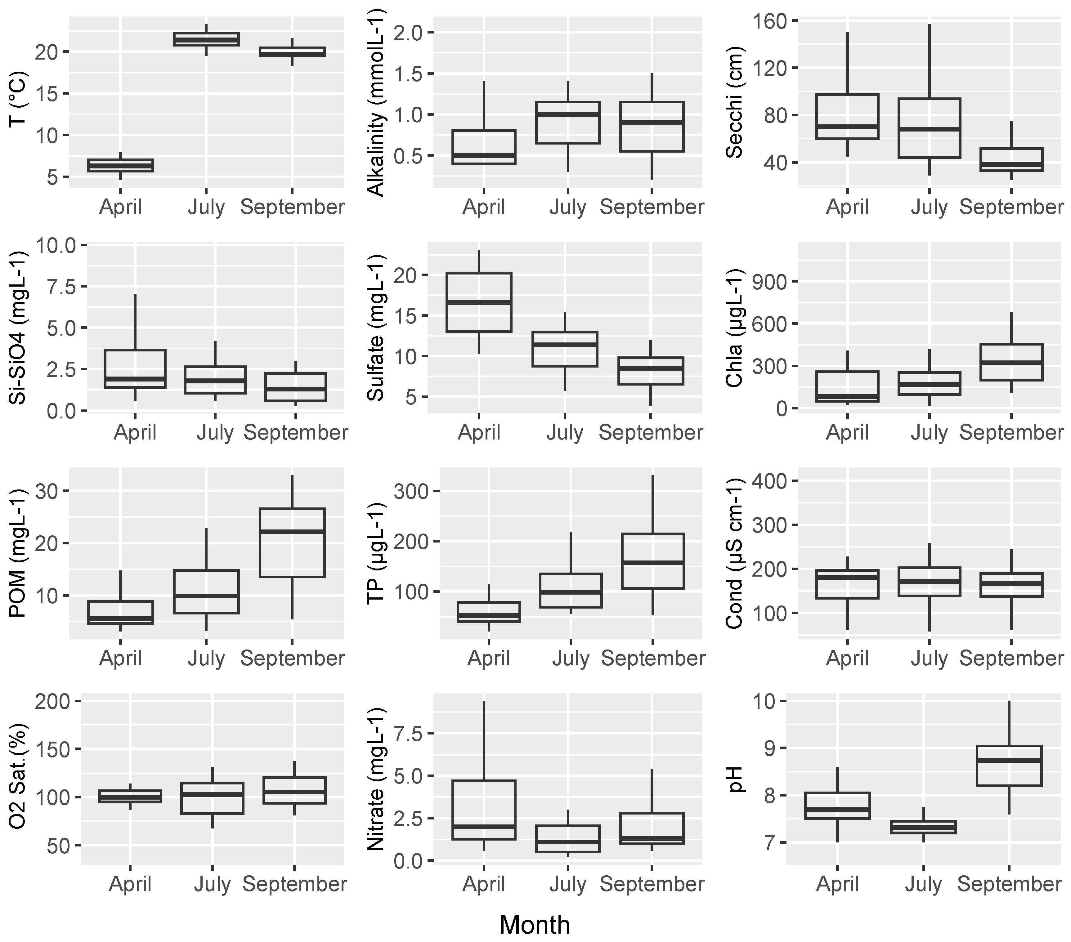
3.1. Environment and Overall Biomass

A summary of characteristic limnological parameters is shown in Figure 1. For attaining insight into habitat differences, we first pre-selected 17 environmental variables out of the 26 analyzed ones based on diurnal stability and to minimize multicollinearity (see also Figure S1). Out of these, Mg²⁺, Cl⁻, total alkalinity, NO₃⁻-N, NPOC, and Secchi-depth accounted most for significant differences between ponds (r = 0.909, BEST permutation routine). We found significant differences between sites (ANOSIM, 9999 permutations, sample statistics R = 0.557, p < 0.001) but not between seasons (R = 0.133, p = 0.320).

Figure 2 combines the cluster analysis based on the BEST-parameters with seven groups identified by the SIMPROF permutation test with the result of NMDS (see also Figure S2). In agreement with ANOSIM, the cluster analysis revealed the main differences between sites rather than between seasons with seven groups classified. Pond 5 (cluster A) and 10 (cluster B) were most dissimilar to the remaining ponds. Pond 2 was grouped in cluster C, and the spring sample of pond 3 was separated from all other samples (F). The autumn sample of three, along with the summer and autumn samples of pond 6 and all samples of 7, were grouped together in cluster D. Another cluster G was pruned by the spring and summer samples of pond 4, and the spring samples of pond 1 and 12. The remaining ponds were grouped together in the large cluster H. Key variables for pruning clusters were identified by LINKTREE analysis (Figure S3). It is evident that cluster A is distinguished from other ponds based on the high amounts of Cl⁻ between 50 and 65 mgL⁻¹. Besides pond 1 (about 40 mgL⁻¹), the other ponds had concentrations < 25 mgL⁻¹. The separation of cluster B from all other ponds was attributed to high NPOC contents, which ranged from 38 to 61 mgL⁻¹; others were mostly <20 mgL⁻¹. Cluster D is defined by its low Mg²⁺ values (1.6 to 3.0 mgL⁻¹) and Cl⁻ amounts < 4.1 mgL⁻¹. The high concentration of NO₃⁻-N (2.1 mgL⁻¹) was responsible for the separation of cluster F from the other ponds, which had amounts < 1.3 mgL⁻¹. Cluster G was defined by Secchi-depth readings between 1.2 and 1.6 m, with the Secchi disc in pond 4 reaching the bottom.

Chl-a, as a proxy for algal biomass, indicated significant differences among seasons (Kruskal–Wallis test, p < 0.001), with an increase from spring to autumn (Dunn-test, p = 0.018) (Figure 5). Chl-a maxima were recorded in 4 out of 15 fishponds in spring, the other peaked in September (Figure S4), with a maximum recorded in pond 2 with 1125 µgL⁻¹. Other Chl-a values ranged between 17 and 803 µgL⁻¹. The results indicate eutrophicated conditions (Figure 3). In agreement, TSI increased from 59 to 71 in spring to 80 to 93 in autumn and classified the ponds as mid-eutrophic to hypertrophic. To identify the parameters coinciding with Chl-a, we performed a regression analysis. First, a group of 11 independent variables that are typically acknowledged to affect microalgae growth was chosen. TP showed the highest and positive relation to algal biomass, while NH₄⁺, conductivity and grazing had negative loadings, with conductivity showing the least effect (Figure 4). NO₃⁻-N, SiO₄, NPOC, IC, temperature, Secchi-depth, and pond area did not contribute significantly to the model and thus were not considered for the final model.

Figure 3. A log–log transformed trophic diagram showing the trophic levels of fishponds with trophic status thresholds according to Forsberg and Ryding.

Figure 3. A log–log transformed trophic diagram showing the trophic levels of fishponds with trophic status thresholds according to Forsberg and Ryding.

Figure 4. Correlation diagram of measured Chlorophyll-a versus predicted Chlorophyll-a computed by backward stepwise regression (r = 0.76, n = 45).

Figure 4. Correlation diagram of measured Chlorophyll-a versus predicted Chlorophyll-a computed by backward stepwise regression (r = 0.76, n = 45).

Figure 5. Mean group contribution to overall algal biomass (n = 15 for each group/season).

Figure 5. Mean group contribution to overall algal biomass (n = 15 for each group/season).

The median of RUE_TP was 1.94 (n = 45) and that of RUE_TN 0.12, with no significant differences between seasons (Kruskal–Wallis test, RUE_TP p = 0.433; RUE_TN p = 0.231). TN/TP ratios were mostly in the range between 10 and 30 with higher ratios during spring compared to summer and autumn (Kruskal–Wallis test p = 0.005).

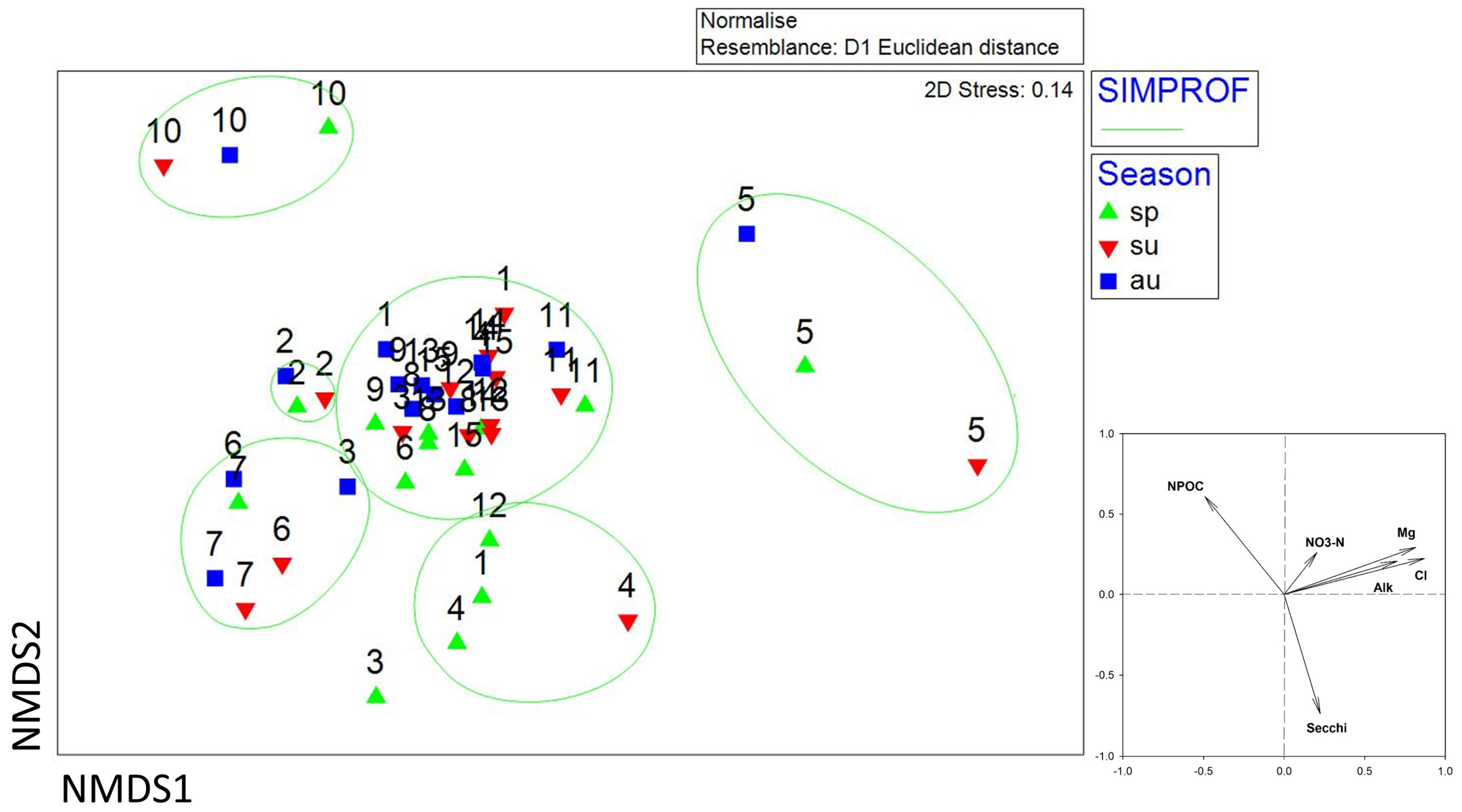
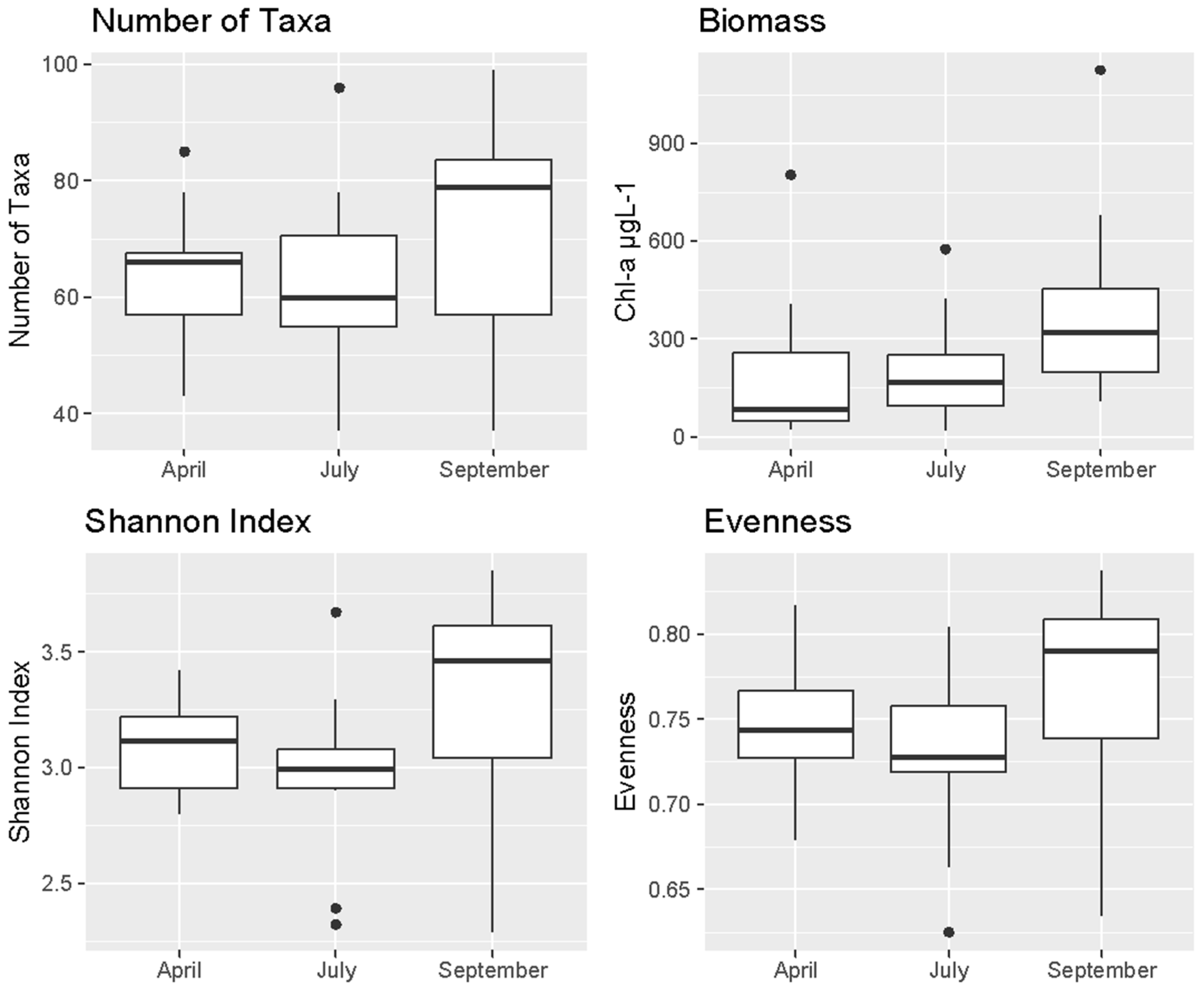
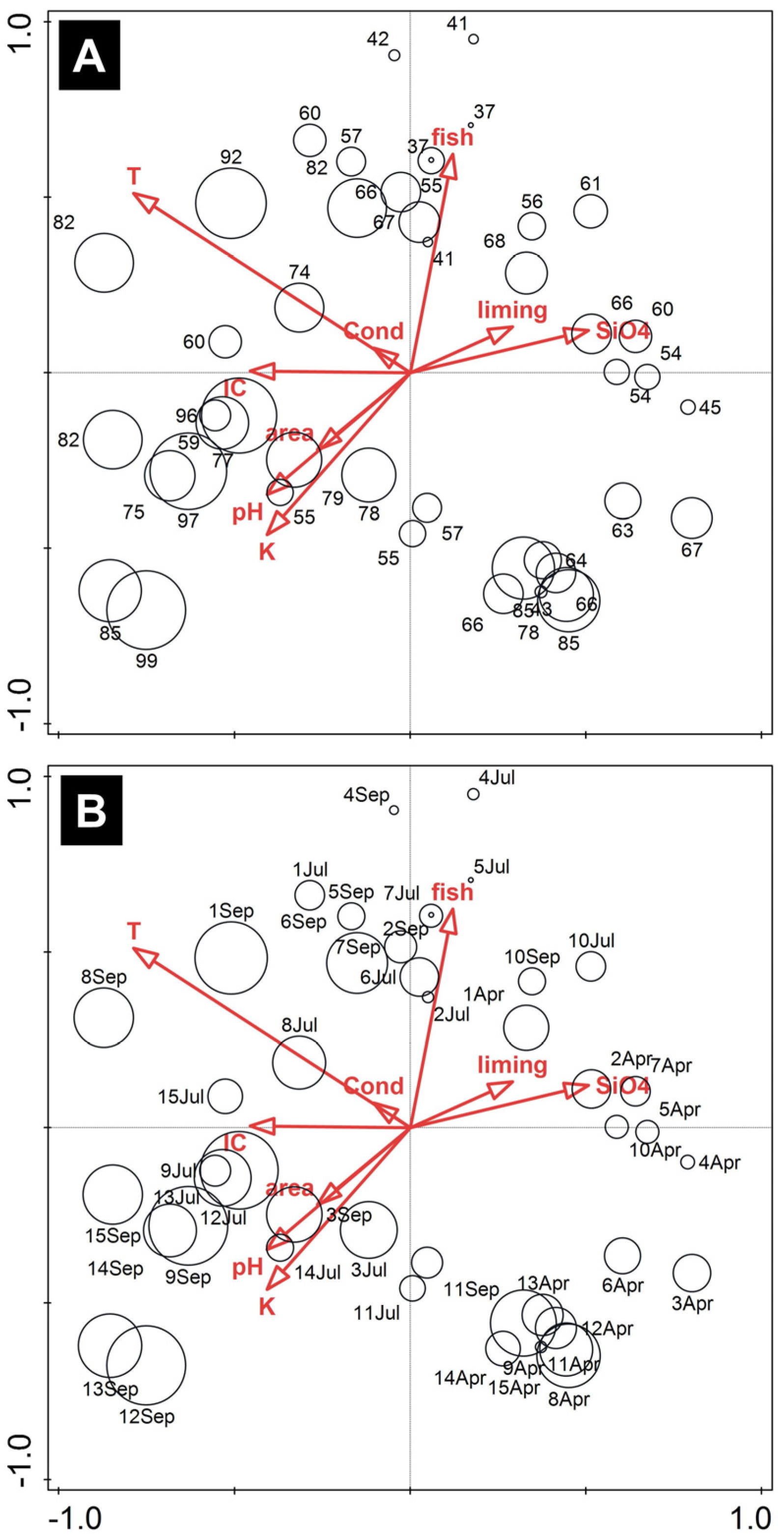
3.2. Algal Community

In terms of biomass, Chrysophyceae and green algae were co-dominant in the colder season, followed by Bacillariophyceae. During the warmer seasons, Chrysophyceae lost in importance for the expense of green algae (Figure 5). A comparable pattern was found with relative abundance estimations with diatoms and green algae co-dominant in spring, followed by Chrysophyceae. Cyanobacteria abundance increased in summer and autumn, but this group was never dominating the biomass. Other groups were less present.

Overall, 462 phytoplankton taxa could be identified. Bacillariophyceae had the highest taxa number with 207 in total, followed by green algae (Chloro- and Streptophyta; 157), Euglenophyta (39), Cyanobacteria (36), Chrysophyceae (16), Xanthophyceae (4), and Dinophyta (2). The Raphidophyceae was represented by only one species (Figure S5). For diversity, the mean H′ and E were high in spring (Average: H′ = 3.10; E = 0.75), with a tendency to decrease during summer (Average: H′ = 2.98; E = 0.72). This was followed by a significant increase in autumn (Average: H′ = 3.29; E = 0.77; posthoc TukeyHSD p = 0.046; Figure 6). The highest H′ and E were observed in pond 12 in autumn (99 taxa, H = 3.85, E = 0.84) and lowest in pond 2 in autumn (37 taxa, H = 2.29, E = 0.63) and pond 4 during summer (41 taxa, H = 2.32, E = 0.63; Table S1).

The main use of the ponds (groups recreation versus aquaculture) revealed significant differences in the algae community (PERMANOVA, p = 0.0001,

Table 2. Summary table of the PERMANOVA results based on relative taxa. Two groups were defined a priori: managed ponds (1,2, 4–9, 12–15) and ponds used for recreation (3, 10, 11). Factors were stocking and seasons. Significance level is assumed with p = 0.05; significant differences between groups are highlighted in bold.

Source	df	SS	MS	Pseudo-F	p (perm)	Unique perms
season	2	10,140	5070.2	2.5428	0.0001	9870
stock	1	6505.5	6505.5	3.2626	0.0001	9862
season x stock	2	2457.7	1228.8	0.61629	0.9954	9836
Res	39	77,763	1993.9
Total	44	1.04 × 105
Pairwise Tests for	Season			t	p(perm)	Unique perms
spring–summer				1.6764	0.0001	9897
spring–autumn				1.9395	0.0001	9892
summer–autumn				1.0859	0.2233	9900

). Also, between seasons, significant differences were found (PERMANOVA, p = 0.0001). Pairwise tests between seasons demonstrated that spring was different from both warmer seasons (p = 0.0001), whereas the warmer seasons showed no significant differences to each other (p = 0.2233). Indicator species analysis revealed a few indicative species for groups recreation and aquaculture, although with comparatively low indicator values, the same for seasons (

Table 3. Indicator species significantly assigned with groups “use” and “season” (p < 0.05) and indicator values (IV) > 60%. An indicator value is the statistical value representing the strength of the association, ranging from 0 to 100%.

Taxon	Group	IV	Mean	St.Dev
Pseudopediastrum boryanum	aquaculture	79	56.4	5.63
Craticula cuspidata	aquaculture	63	37.5	9.15
Eudorina elegans	aquaculture	61	38.1	9.09
Navicula cryptocephala	aquaculture	61	44.4	8.04
Desmodesmus armatus var. longispina	recreation	65	45.1	9.31
Aulacoseira muzzanensis	recreation	63	45.1	9.51
Ankistrodesmus arcuatus	spring	82	22.7	6.68
Pinnilaria viridis	spring	78	22.1	7.46
Cymatopleura solea	spring	67	26.6	8.89
Ulnaria ulna	spring	65	19.5	7.32
Asterionella formosa	spring	65	37.1	6.24
Dinobryon cylindricum	spring	60	15.4	6.14
Trachelomonas volvocina	autumn	84	20.2	6.67
Scenedesmus obtusus f. disciformis	autumn	61	25.3	6.86

).

RDA resulted in a significant model with explanatory variables accounting for 40% of the total variation in the community structure (

Table 4. Summary table of the redundancy analysis (RDA) results based on relative taxa abundances displays the eigenvalues, cumulative explained variation from axes 1 to 4, and pseudo-canonical correlation between environmental variables and axes. The total variation in the data is 6537.644, of which the explanatory variables account for 40.16%. The adjusted explained variation is 24.77%, indicating that the selected environmental variables account for a significant proportion of the variation in the relative taxa abundances.

Statistic	Axis 1	Axis 2	Axis 3	Axis 4
Eigenvalues	0.12	0.08	0.06	0.04
Explained variation (cumulative)	11.69	19.45	25.17	29.44
Pseudo-canonical correlation	0.94	0.95	0.94	0.91
Explained fitted variation (cumulative)	29.12	48.42	62.67	73.31
p value	0.0001	0.0001	0.0001	0.0003

). Water temperature had the highest explanatory value with consistent simple and conditional effects (9.8), followed by K⁺ (6.4). Other variables with significant loadings were DIC, SiO₄-Si, fish stock, liming, pH value, pond area, and conductivity in decreasing order (

Table 5. Contributions of significant explanatory variables to the RDA model, including both the simple and conditional effects of each environmental variable. Abbreviations of variables: Temp, temperature; K⁺, Potassium; DIC, dissolved inorganic carbon; fish, fish stock amount (piece ha⁻¹); liming, carbonate addition; area, pond area in hectare; Cond, conductivity.

Name	Simple	Conditional	Pseudo-F	p	p(adj)
Temp	9.8	9.8	4.7	0.0001	0.0009
K+	6.4	6.3	3	0.0001	0.0009
DIC	6.2	3.1	2.9	0.0002	0.0012
SiO4	5.9	4.4	2.7	0.0001	0.0009
fish	5.5	5.3	2.5	0.0003	0.0015
liming	5.2	2.9	2.4	0.0004	0.0016
pH	5	2.9	2.2	0.0009	0.0027
area	4.7	3.4	2.1	0.0013	0.0027
Cond	4.3	2	1.9	0.0035	0.0035

). Temperature, K⁺, and pH turned out as key factors for taxa richness (Figure 7). We found a distinct seasonal pattern: in spring, ponds 2, 4, 5, 7, and 10 exhibited lower taxa richness between 45 to 66, strongly associated with higher SiO₄-Si levels but negatively related to DIC. Conversely, ponds with greater species richness ranging from 55 to 99 in the warmer seasons were related to higher pH, DIC, K⁺ levels, and pond area but negatively correlated with SiO₄-Si concentrations. Additionally, pond 10 was highly negatively related to pH, indicating that pH played a pivotal role in shaping the taxa number in that specific pond. Moreover, higher fish stocks were related to lower taxa numbers.

The composition of specific algal groups exhibited a pronounced seasonal pattern (Figure 8). In April, diatoms constituted most of the taxa recorded, accounting for an average of 56%, followed by green algae (30%). Cyanobacteria played a minor role. As summer approached, green algae became more diverse, accounting for an average of 49% of the taxa number. Diatoms were still a major component in summer (31%), and Cyanobacteria and Euglenophyta gained in importance (11% and 5% on average, respectively). In autumn, green algae accounted for a significant proportion of the taxa found in samples, averaging at 46%. Cyanobacteria and Euglenophyta further gained in importance compared to spring and summer (13% and 9%). It is worth noting that the category “remain” includes Xanthophyceae, Dinophyta, and Raphidophyceae. The proportion of this category appears high in pond 2 during summer and autumn due to the overall low total species count in this water body.

The abundant species inventory of the ponds was comparable. In spring, Bacillariophyceae were dominated by common species such as Aulacoseira ambigua (Grunow) Simonsen, A. granulata (Ehrenb.) Simonsen, Ulnaria acus (Kütz.) Aboal, Asterionella formosa Hassall, and Nitzschia acicularis (Kütz.) W.Smith. Green algae were represented by high numbers of Scenedesmus quadricauda (Turpin) Brébisson, Pseudopediastrum boryanum (Turpin) E.Hegewald, and Monoraphidium spp. In summer, Monoraphidium spp. decreased for the expense of other species such as Pediastrum duplex Meyen, Eudorina elegans Ehrenb., Lemmermannia komarekii (Hindák) C.Bock and Krienitz, Coelastrum microporum Nägeli, and Hindakia tetrachotoma (Printz) C.Bock, Pröschold, and Krienitz. Volvox aureus Ehrenb. was most abundant in autumn. The abundance of Bacillariophyceae was less than in spring but with a comparable species inventory.

Cyanobacteria was less abundant in spring, with Limnothrix redekei (Goor) Meffert being the most frequent species. During summer and autumn, Cyanobacteria gradually increased. Aside from Limnothrix, other species were observed more frequently in summer, e.g., Microcystis aeruginosa (Kützing) Kützing, Planktothrix agardhii (Gomont) Anagnostidis and Komárek, and Snowella lacustris (Chodat) Komárek and Hindák. In September, Aphanocapsa incerta (Lemmerm.) G.Cronberg and Komárek, Planktothrix agardhii (Gomont) Anagnostidis and Komárek, and Dolichospermum viguieri (Denis and Frémy) Wacklin, L.Hoffmann, and Komárek were also observed.

The abundance of Chrysophyceae was highest in spring, mainly comprising Dinobryon spp. and Synura petersenii Korshikov. During summer and autumn, Dinobryon almost disappeared; instead, Mallomonas cf. ploesslii Perty became abundant. Dinophyta were represented by Ceratium hirundinella (O.F.Müller) Dujardin, which was, however, not detected in spring. Euglenophytes were not common in spring. In summer, Euglena texta (Dujardin) Hübner and Phacus longicauda Ehrenb. were identified. A significant increase in Trachelomonas volvocina (Ehrenb.) Ehrenb. abundance was observed in September. Gonyostomum semen (Ehrenberg) Diesing was the only Raphidophyceae detected, starting to grow in summer, with the highest abundance observed in September. Xanthophyceae were always present, although very rare, mainly consisting of Centritractus belonophorus (Schmidle) Lemmerm. and Ophiocytium capitatum Wolle.

The biplot of RDA with environmental variables and phytoplankton taxa with the best fit to the model is shown in Figure 9 (for correlation coefficients with the corresponding explanatory variables see Table S2). All Cyanobacteria considered in the best fit model were highly related with increased water temperature, pH, K⁺, and DIC concentrations (Table S2). These species thrived in larger ponds with lower fish stocking and reduced SiO₄-Si concentrations (exception is Planktothrix agardhii with a preference for small ponds). Green algae show a similar pattern with a preference for higher water temperatures and DIC but lower SiO₄-Si concentrations. Particularly, Eudorina elegans performed well at high DIC levels during summer. Most diatoms and the colony-forming Chrysophyceae Dinobryon cylindricum O.E.Imhof showed a preference for lower water temperature. In contrast, the dinoflagellate Ceratium hirundinella preferred large ponds during the summer season, coupled with low SiO₄-Si.

4. Discussion

Based on chemical parameters, Chl-a and TSI, the ponds were classified as highly eutrophicated systems. Both TN and TP concentrations raised in the warmer seasons but TP increase was more pronounced (mean spring–summer autumn TP = 58, 122, 158 µgL⁻¹, TN = 1.5, 1.6, 2.0 mgL⁻¹), causing a seasonal TN/TP drop from 30 in spring to approximately 15 in summer and autumn. A decrease in the TN/TP ratio in the course of the growing season was also observed in a survey in nearby Czech fishponds [103]. TN/TP ratios categorize the ponds as nutrient-balanced water bodies [79]. Although the regression model of Chl-a does not imply causation, the highly significant and positive loading of TP might be a hint for potential phosphorus limitation, which agrees to other studies [14,103]. RUE_TP (median 1.94, n = 45, converted to lnRUE_C/TP = 4.16, lnRUE_biomass/TP = 12.87) was in the upper range of other highly eutrophicated water bodies [104,105,106] and can be explained by the comparatively high biodiversity occupying various ecological niches [70]. We were not able to verify a significant relationship between diversity parameters and RUE_TP (Spearman rank correlation for taxa number p = 0.37, H′ p = 0.48, E p = 0.32), probably due to the short eutrophication gradient considered in the current study.

Pond systems enrich the diversity of the landscape [107] and provide various ecosystem services [108]. Biodiversity and habitat heterogeneity are, however, impaired by eutrophication [109,110,111], which curtails the contribution to biological diversity. In contrast to our expectations, we recorded unexpectedly high taxa numbers in the ponds with > 100 algae genera, which we mainly attribute to organic farming. In addition, the identification method applied provides much more detailed insights into biodiversity compared to identifications with counting chambers. This, however, makes comparisons with other studies difficult, even on the genus level, e.g., for diatoms. Our numbers considerably exceed the findings of Zhang et al. [112] regarding phytoplankton richness along a productivity gradient. Zhang et al. [112] found in lake water with a Chl-a amount around 200 µgL⁻¹ species richness < 40, with even lower species number at higher Chl-a values. Another study on species richness of the whole pelagic community in an eutrophic reservoir in Brazil resulted in an average species richness of 60 [113]. A thorough survey along 83 eutrophic fishponds in eastern France, lasting for two years with 22 sampling dates, recorded around 15 to 45 taxa per pond with a total of 30 phytoplankton genera [114]. Another detailed study on phytoplankton succession along a series of nearby fishponds in the Czech Republic provided mainly very abundant taxa but did not list the taxa number [14].

We recorded 14 species in at least 8 out of 15 sampled fishponds in each season, with all frequent taxa belong to diatoms and green algae, such as Aulacoseira, Pediastrum, and Scenedesmus (Figure S6). Among these taxa, 12 are known to occur in eu- to hypertrophic water bodies [115,116]. In agreement with previous studies [14,15,36,55,117], colonial Cyanobacteria Microcystis aeruginosa, Aphanocapsa spp., and filamentous forms Planktothrix agardhii, Limnothrix redekei, Dolichospermum spp., and Aphanizomemon sp. increased in summer, although the community was still dominated by green algae and diatoms. The higher occurrence is partly attributed to the benefits conferred by gas vesicles of certain Cyanobacteria, enabling them to adjust their buoyancy and move vertically toward the water surface for photosynthesis, especially at higher turbidity [51,118]. Cyanobacteria also have a distinct advantage in low-light conditions because they can sustain biomass with lower energy than eukaryotic algae [119,120,121]. Also, higher temperatures promote Cyanobacteria development [39,122,123,124]. During summer, increased fish activity may reduce large herbivorous zooplankton preying on edible colonial cyanobacterial populations, thus promoting cyanobacterial blooms [125,126,127], as previously discussed. Increased frequency of filamentous Cyanobacteria like P. agardhii and L. redekei in the current study aligns with the results of numerous studies on turbid eu- to hypertrophic shallow lakes [128,129,130,131,132,133,134] and fishponds [14,135,136,137,138,139]. Meanwhile, various studies have proved that certain strains of P. agardhii produce notably high quantities of microcystins and other potentially toxic metabolites [140,141,142], which have the potential to adversely affect fish and crustaceans. To determine whether such phenomena are also present in the studied fishponds, further investigation is required. Increased frequency of M. aeruginosa and Dolichospermum spp. further point to increased eutrophication levels during warmer seasons [143], which was confirmed in our study also by higher TSI.

Although the focus of the current study was not on phytoplankton succession (the seasonal sampling is like a snapshot of the community pattern), some general conclusions can be drawn. To our knowledge, algae community shifts in eutrophicated fishponds do not occur in short time intervals throughout the year. It is more like a seasonal pattern, which can be concluded from studies with short sampling intervals [14,44,137]. Both biomass and relative abundance revealed an algal community dominated by Ochrophyta and green algae throughout the survey. This finding is consistent with a study conducted 50 years ago suggesting that Cyanobacteria were less abundant compared to other algal groups in fishponds that did not receive fertilization [144]. Also, in agreement with our findings, Wawrik [145] and Kopp et al. [146] found dominance of Chrysophyceae during spring for newly constructed ponds. Other studies list diatoms dominating in spring as well, followed by green algae during the summer [143,147]. This pattern can be explained by the shallow nature of the fishponds and the predominant cultivation of common carp, which causes bioturbation, potentially facilitating the upward movement of algae lacking buoyancy-regulating mechanisms. It may also be related to the transition of fishpond management from conventional to organic farming, as it is mitigating excessive nutrient loading. This approach fosters a balanced population and size diversity of zooplankton that feed on algae [54,148] in contrast to conventional farming with low crustacean abundances causing imbalances in the trophic cascade [67]. Organic farming enhances algal diversity and moreover minimizes the risk dominance of Cyanobacteria colonies that large zooplankton typically avoid [50,149]. The observed pattern is comparable to shallow-lakes systems with high fish densities, as described in the expanded PEG-model [150]. The distinct seasonal pattern is in line with existing studies and primarily attributed to water temperature [136,139,151,152]. Other researchers have suggested pH, TP, and TN as key variables for seasonal shifts [14,153,154].

The presence of fish stocking does not necessarily lead to detrimental ecosystem conditions. On the other side, fishponds that have lost their ecological functionality may struggle to recover even after discontinuing fish stocking. In the Zámecký fishpond studied by Radojicic et al. [143], a remarkable occurrence of Cyanobacteria was still observed 10 years after fish production was stopped, indicating the ecological memory of these water bodies.

Especially during warmer seasons, we identified a variety of taxa that are typical inhabitants of shallow nutrient-enriched turbid lakes and ponds. We therefore assume that ongoing climate change has considerable effects on the ecological balance of fishponds. Rising temperature combined with high nutrient load may cause a sharp reduction in the diversity of algae [155,156,157,158]. This scenario might lead to prolonged Cyanobacteria blooms in the future due to their competitive advantage at such conditions. As phytoplankton forms the basis of aquatic food webs, any alterations in the composition of algae could subsequently trigger changes in the entire pond ecosystem. This, in turn, would impact all organisms therein, as well as the other organisms including humans that rely on the pond for various ecological services.

5. Conclusions

Waldviertel fishponds exhibit higher phytoplankton species diversity compared to other hypertrophic systems. Although Cyanobacteria were typical of hypertrophic systems, they were frequent, especially during the warmer seasons, and they did not dominate the community. Instead, chrysophytes, green algae, and diatoms prevailed in spring, followed by green algae during summer. Each of the ponds offers unique environmental conditions contributing to biodiversity at a regional scale. Although the algal community pattern follows a temporal pattern rather than a spatial one on a regional scale, this heterogeneity is of special importance, as fishponds are strongly interconnected to the terrestrial environment, e.g., via emerging insects and waterfowl. Water temperature, as a key variable, highlights the potential effects of future climate change on these aquatic systems. We propose long-term monitoring, which allows timely adjustments to management practices and the development of viable strategies to maintain the health and sustainability of these peculiar aquatic ecosystems.

References

1. Adámek, Z.; Linhart, O.; Kratochvíl, M.; Flajšhans, M.; Randak, T.; Policar, T.; Masojídek, J.; Kozák, P. Aquaculture the Czech Republic in 2012: Modern European prosperous sector based on thousand-year history of pond culture. Aquac. Eur. 2012, 37, 5–14. [Google Scholar]
2. Bauer, C. Waldviertler Teiche. Denisia 2014, 33, 157–166. [Google Scholar]
3. Bezzel, E. Vögel in der Kulturlandschaft; Verlag Eugen Ulmer: Stuttgart, Germany, 1982. [Google Scholar]
4. Steiner, E. Die Brutzeit bei Wasservögeln am Beispiel der Fischteiche des Waldviertels; Kataloge des OÖ. Landesmuseums: Linz, Austria, 1987; pp. 55–63. [Google Scholar]
5. Fehlinger, L.; Misteli, B.; Morant, D.; Juvigny-Khenafou, N.; Cunillera-Montcusí, D.; Chaguaceda, F.; Stamenković, O.; Fahy, J.; Kolář, V.; Halabowski, D.; et al. The ecological role of permanent ponds in Europe: A review of dietary linkages to terrestrial ecosystems via emerging insects. Inland Waters 2023, 13, 30–46. [Google Scholar] [CrossRef]
6. Fehlinger, L.; Mathieu-Resuge, M.; Pilecky, M.; Parmar, T.P.; Twining, C.W.; Martin-Creuzburg, D.; Kainz, M.J. Export of dietary lipids via emergent insects from eutrophic fishponds. Hydrobiologia 2023, 850, 3241–3256. [Google Scholar] [CrossRef] [PubMed]
7. Matzinger, T.M.E. Teiche in der Landschaft: Bedeutung, Funktionen und Gefährdung; Bundesamt für Wasserwirtschaft, Ökologische Station Waldviertel: Wien, Austria, 2014. [Google Scholar]
8. Poschlod, P.; Rosbakh, S. Mudflat species: Threatened or hidden? An extensive seed bank survey of 108 fish ponds in Southern Germany. Biol. Conserv. 2018, 225, 154–163. [Google Scholar] [CrossRef]
9. Knittler, H. Teiche als Konjunkturbarometer? Das Beispiel Niederösterreich. Water Manag. Mediev. Rural Econ. RURALIA 2005, 5, 208–221. [Google Scholar]
10. Wawrik, F. Seltene Diatomeen aus Teichen des N.Ö. Waldviertels. Nova Hedwig. Beih. 1970, 31, 443–448. [Google Scholar] [CrossRef]
11. Wawrik, F. Seltene “-Algen”︁ und Nannoplankter aus Teichen des Waldviertels (Nieder-Österreich). Int. Rev. Gesamten Hydrobiol. Hydrogr. 1974, 59, 247–254. [Google Scholar] [CrossRef]
12. Wawrik, F. Vergleichende Braunwasser-Teichstudien im niederösterreichischen Waldviertel. Hydrobiologia 1972, 39, 17–82. [Google Scholar] [CrossRef]
13. Radojičić, M.; Šorf, M.; Müllerová, B.; Kopp, R. Phytoplankton-zooplankton coupling in a cascade of hypertrophic fishponds. J. Limnol. 2023, 82, 2145. [Google Scholar] [CrossRef]
14. Ivanova, A.P.; Vrba, J.; Potužák, J.; Regenda, J.; Strunecký, O. Seasonal Development of Phytoplankton in South Bohemian Fishponds (Czechia). Water 2022, 14, 1979. [Google Scholar] [CrossRef]
15. Radojicic, M.; Kopp, R. Dynamic of the phytoplankton community in eutrophic fishponds. MendelNet 2016, 2016, 352–357. [Google Scholar]
16. Radojičić, M.; Kopp, R.; Müllerová, B.; Šorf, M. The Effect of Fish Production and Environmental Factors on Phytoplankton in Hypertrophic Fishponds. Acta Univ. Agric. Silvic. Mendel. Brun. 2022, 70, 397–406. [Google Scholar] [CrossRef]
17. Rahman, M.M. Role of common carp (Cyprinus carpio) in aquaculture production systems. Front. Life Sci. 2015, 8, 399–410. [Google Scholar] [CrossRef]
18. Liu, Q.-G.; Chen, Y.; Li, J.-L.; Chen, L.-Q. The food web structure and ecosystem properties of a filter-feeding carps dominated deep reservoir ecosystem. Ecol. Model. 2007, 203, 279–289. [Google Scholar] [CrossRef]
19. Baxa, M.; Musil, M.; Kummel, M.; Hanzlík, P.; Tesařová, B.; Pechar, L. Dissolved oxygen deficits in a shallow eutrophic aquatic ecosystem (fishpond)—Sediment oxygen demand and water column respiration alternately drive the oxygen regime. Sci. Total Environ. 2021, 766, 142647. [Google Scholar] [CrossRef]
20. Chen, W.; Li, T.; Du, S.; Chen, H.; Wang, Q. Microalgal polyunsaturated fatty acids: Hotspots and production techniques. Front. Bioeng. Biotechnol. 2023, 11, 1146881. [Google Scholar] [CrossRef]
21. Brett, M.; Müller-Navarra, D. The role of highly unsaturated fatty acids in aquatic foodweb processes. Freshw. Biol. 1997, 38, 483–499. [Google Scholar] [CrossRef]
22. Patil, V.; Reitan, K.I.; Knutsen, G.; Mortensen, L.M.; Källqvist, T.; Olsen, E.F.; Vogt, G.; Gislerød, H.R. Microalgae as source of polyunsaturated fatty acids for aquaculture. Curr. Top. Plant Biol. 2005, 6, 57–65. [Google Scholar]
23. Pilecky, M.; Mathieu-Resuge, M.; Závorka, L.; Fehlinger, L.; Winter, K.; Martin-Creuzburg, D.; Kainz, M.J. Common carp (Cyprinus carpio) obtain omega-3 long-chain polyunsaturated fatty acids via dietary supply and endogenous bioconversion in semi-intensive aquaculture ponds. Aquaculture 2022, 561, 738731. [Google Scholar] [CrossRef]
24. Mráz, J.; Máchová, J.; Kozák, P.; Pickova, J. Lipid content and composition in common carp—Optimization of n-3 fatty acids in different pond production systems. J. Appl. Ichthyol. 2012, 28, 238–244. [Google Scholar] [CrossRef]
25. Jaworski, N.A.; Howarth, R.W.; Hetling, L.J. Atmospheric deposition of nitrogen oxides onto the landscape contributes to coastal eutrophication in the northeast United States. Environ. Sci. Technol. 1997, 31, 1995–2004. [Google Scholar] [CrossRef]
26. Peltzer, P.M.; Lajmanovich, R.C.; Sánchez-Hernandez, J.C.; Cabagna, M.C.; Attademo, A.M.; Bassó, A. Effects of agricultural pond eutrophication on survival and health status of Scinax nasicus tadpoles. Ecotoxicol. Environ. Saf. 2008, 70, 185–197. [Google Scholar] [CrossRef] [PubMed]
27. Breukelaar, A.W.; Lammens, E.H.R.R.; Breteler, J.G.P.K.; Tatrai, I. Effects of benthivorous bream (Abramis brama) and carp (Cyprinus carpio) on sediment resuspension and concentrations of nutrients and chlorophyll a. Freshw. Biol. 1994, 32, 113–121. [Google Scholar] [CrossRef]
28. Meijer, M.L.; De Haan, M.W.; Breukelaar, A.W.; Buiteveld, H. Is reduction of the benthivorous fish an important cause of high transparency following biomanipulation in shallow lakes? In Biomanipulation Tool for Water Management; Springer: Dordrecht, The Netherlands, 1990; pp. 303–315. [Google Scholar]
29. Driver, P.D.; Closs, G.P.; Koen, T. The effects of size and density of carp (Cyprinus carpio L.) on water quality in an experimental pond. Arch. Hydrobiol. 2005, 163, 117–131. [Google Scholar] [CrossRef]
30. Prescott, K.L.; Tsanis, I.K. Mass balance modelling and wetland restoration. Ecol. Eng. 1997, 9, 1–18. [Google Scholar] [CrossRef]
31. Roy, K.; Vrba, J.; Kuebutornye, F.K.A.; Dvorak, P.; Kajgrova, L.; Mraz, J. Fish stocks as phosphorus sources or sinks: Influenced by nutritional and metabolic variations, not solely by dietary content and stoichiometry. Sci. Total Environ. 2024, 938, 173611. [Google Scholar] [CrossRef]
32. Roy, K.; Vrba, J.; Kajgrova, L.; Mraz, J. The concept of balanced fish nutrition in temperate European fishponds to tackle eutrophication. J. Clean. Prod. 2022, 364, 132584. [Google Scholar] [CrossRef]
33. Hargreaves, J.A. Nitrogen biogeochemistry of aquaculture ponds. Aquaculture 1998, 166, 181–212. [Google Scholar] [CrossRef]
34. Durborow, R.M.; Crosby, D.M.; Brunson, M.W. Ammonia in fish ponds. J. Fish. Res. Board Can. 1997, 32, 2379–2383. [Google Scholar]
35. Zhao, J.; Zhang, M.; Xiao, W.; Jia, L.; Zhang, X.; Wang, J.; Zhang, Z.; Xie, Y.; Pu, Y.; Liu, S.; et al. Large methane emission from freshwater aquaculture ponds revealed by long-term eddy covariance observation. Agric. For. Meteorol. 2021, 308–309, 108600. [Google Scholar] [CrossRef]
36. Sevrin-Reyssac, J.; Pletikosic, M. Cyanobacteria in fish ponds. Aquaculture 1990, 88, 1–20. [Google Scholar] [CrossRef]
37. Lakshmikandan, M.; Li, M.; Pan, B. Cyanobacterial Blooms in Environmental Water: Causes and Solutions. Curr. Pollut. Rep. 2024, 10, 606–627. [Google Scholar] [CrossRef]
38. Huisman, J.; Codd, G.A.; Paerl, H.W.; Ibelings, B.W.; Verspagen, J.M.H.; Visser, P.M. Cyanobacterial blooms. Nat. Rev. Microbiol. 2018, 16, 471–483. [Google Scholar] [CrossRef]
39. Paerl, H.W.; Huisman, J. Blooms like it hot. Science 2008, 320, 57–58. [Google Scholar] [CrossRef]
40. Rigosi, A.; Carey, C.C.; Ibelings, B.W.; Brookes, J.D. The interaction between climate warming and eutrophication to promote cyanobacteria is dependent on trophic state and varies among taxa. Limnol. Oceanogr. 2014, 59, 99–114. [Google Scholar] [CrossRef]
41. Kosten, S.; Huszar, V.L.M.; Bécares, E.; Costa, L.S.; van Donk, E.; Hansson, L.-A.; Jeppesen, E.; Kruk, C.; Lacerot, G.; Mazzeo, N.; et al. Warmer climates boost cyanobacterial dominance in shallow lakes. Glob. Change Biol. 2012, 18, 118–126. [Google Scholar] [CrossRef]
42. Potužák, J.; Hůda, J.; Pechar, L. Changes in fish production effectivity in eutrophic fishponds—Impact of zooplankton structure. Aquac. Int. 2007, 15, 201–210. [Google Scholar] [CrossRef]
43. Oliver, R.L.; Hamilton, D.P.; Brookes, J.D.; Ganf, G.G. Physiology, Blooms and Prediction of Planktonic Cyanobacteria. In Ecology of Cyanobacteria II: Their Diversity in Space and Time; Whitton, B.A., Ed.; Springer: Dordrecht, The Netherlands, 2012; pp. 155–194. [Google Scholar]
44. Pechar, L. Long-term changes in fish pond management as’ an unplanned ecosystem experiment’: Importance of zooplankton structure, nutrients and light for species composition of cyanobacterial blooms. Water Sci. Technol. 1995, 32, 187–196. [Google Scholar] [CrossRef]
45. Huang, Y.; Hong, J.; Liang, C.; Li, G.; Shen, L.; Zhang, H.; Hu, X.; Chen, X. Nitrogen limitation affects the sinking property of Microcystis by promoting carbohydrate accumulation. Chemosphere 2019, 221, 665–671. [Google Scholar] [CrossRef]
46. Ji, Y.; Shi, W.; Qin, B. An indispensable role of overlying water in nitrogen removal in shallow lakes. Sci. Total Environ. 2024, 923, 171487. [Google Scholar] [CrossRef] [PubMed]
47. Zhu, L.; Shi, W.; Zhou, J.; Yu, J.; Kong, L.; Qin, B. Strong turbulence accelerates sediment nitrification-denitrification for nitrogen loss in shallow lakes. Sci. Total Environ. 2021, 761, 143210. [Google Scholar] [CrossRef] [PubMed]
48. Brunson, M.W.; Lutz, C.G.; Durborow, R.M. Algae Blooms in Commercial Fish Production Ponds; Southern Regional Aquaculture Center: Stoneville, MS, USA, 1994. [Google Scholar]
49. Landsberg, J.H.; Hendrickson, J.; Tabuchi, M.; Kiryu, Y.; Williams, B.J.; Tomlinson, M.C. A large-scale sustained fish kill in the St. Johns River, Florida: A complex consequence of cyanobacteria blooms. Harmful Algae 2020, 92, 101771. [Google Scholar] [CrossRef] [PubMed]
50. Ger, K.A.; Urrutia-Cordero, P.; Frost, P.C.; Hansson, L.-A.; Sarnelle, O.; Wilson, A.E.; Lürling, M. The interaction between cyanobacteria and zooplankton in a more eutrophic world. Harmful Algae 2016, 54, 128–144. [Google Scholar] [CrossRef]
51. Dokulil, M.T.; Teubner, K. Cyanobacterial dominance in lakes. Hydrobiologia 2000, 438, 1–12. [Google Scholar] [CrossRef]
52. Ekvall, M.K.; Urrutia-Cordero, P.; Hansson, L.-A. Linking cascading effects of fish predation and zooplankton grazing to reduced cyanobacterial biomass and toxin levels following biomanipulation. PLoS ONE 2014, 9, e112956. [Google Scholar] [CrossRef]
53. Wunder, W. Das Plankton als wichtiger Bestandteil der Naturnahrung des Karpfens. Methoden der Planktonvermehrung. Osterr. Fisch. 1968, 21, 97–103. [Google Scholar]
54. Schlott, K.; Schlott, G.; Gratzl, G.; Fichtenbauer, M.; Bauer, C. Demand-oriented feeding in carp pond Farming. The settling volume of zooplankton. Zenodo 2023, 35. [Google Scholar] [CrossRef]
55. Drobac, D.; Tokodi, N.; Lujić, J.; Marinović, Z.; Subakov-Simić, G.; Dulić, T.; Važić, T.; Nybom, S.; Meriluoto, J.; Codd, G.A. Cyanobacteria and cyanotoxins in fishponds and their effects on fish tissue. Harmful Algae 2016, 55, 66–76. [Google Scholar] [CrossRef]
56. Malbrouck, C.; Kestemont, P. Effects of microcystins on fish. Environ. Toxicol. Chem. Int. J. 2006, 25, 72–86. [Google Scholar] [CrossRef]
57. Stepanova, N.; Nikitin, O.; Latypova, V.; Kondratyeva, T. Cyanotoxins as a possible cause of fish and waterfowl death in the Kazanka River (Russia). In Proceedings of the International Multidisciplinary Scientific GeoConference-SGEM, Albena, Bulgaria, 2–8 July 2018; pp. 2–8. [Google Scholar]
58. Greer, B.; Maul, R.; Campbell, K.; Elliott, C.T. Detection of freshwater cyanotoxins and measurement of masked microcystins in tilapia from Southeast Asian aquaculture farms. Anal. Bioanal. Chem. 2017, 409, 4057–4069. [Google Scholar] [CrossRef] [PubMed]
59. Varga, D.; Sándor, Z.; Hancz, C.; Csengeri, I.; Jeney, Z.; Papp, Z. Off-flavour compounds in common carp (Cyprinus carpio L.) flesh in context of type of fish pond. Acta Aliment. 2015, 44, 311–315. [Google Scholar] [CrossRef]
60. Abd El-Hack, M.E.; El-Saadony, M.T.; Elbestawy, A.R.; Ellakany, H.F.; Abaza, S.S.; Geneedy, A.M.; Salem, H.M.; Taha, A.E.; Swelum, A.A.; Omer, F.A. Undesirable odour substances (geosmin and 2-methylisoborneol) in water environment: Sources, impacts and removal strategies. Mar. Pollut. Bull. 2022, 178, 113579. [Google Scholar] [CrossRef]
61. Van der Ploeg, M.; Tucker, C.S.; Boyd, C.E. Geosmin and 2-methylisoborneol production by cyanobacteria in fish ponds in the southeastern United States. Water Sci. Technol. 1992, 25, 283–290. [Google Scholar] [CrossRef]
62. van der Ploeg, M.; Boyd, C.E. Geosmin production by cyanobacteria (blue-green algae) in fish ponds at Auburn, Alabama. J. World Aquac. Soc. 1991, 22, 207–216. [Google Scholar] [CrossRef]
63. Pechar, L. Impacts of long-term changes in fishery management on the trophic level water quality in Czech fish ponds. Fish. Manag. Ecol. 2000, 7, 23–31. [Google Scholar] [CrossRef]
64. Søndergaard, M.; Jensen, J.P.; Jeppesen, E. Role of sediment and internal loading of phosphorus in shallow lakes. Hydrobiologia 2003, 506, 135–145. [Google Scholar] [CrossRef]
65. Orihel, D.M.; Baulch, H.M.; Casson, N.J.; North, R.L.; Parsons, C.T.; Seckar, D.C.M.; Venkiteswaran, J.J. Internal phosphorus loading in Canadian fresh waters: A critical review and data analysis. Can. J. Fish. Aquat. Sci. 2017, 74, 2005–2029. [Google Scholar] [CrossRef]
66. Boyd, C.E. Practical Aspects of Chemistry in Pond Aquaculture. Progress. Fish-Cult. 1997, 59, 85–93. [Google Scholar] [CrossRef]
67. Vrba, J.; Šorf, M.; Nedoma, J.; Benedová, Z.; Kröpfelová, L.; Šulcová, J.; Tesařová, B.; Musil, M.; Pechar, L.; Potužák, J.; et al. Top-down and bottom-up control of plankton structure and dynamics in hypertrophic fishponds. Hydrobiologia 2024, 851, 1095–1111. [Google Scholar] [CrossRef]
68. Schlott, K. Die Planktische Naturnahrung und Ihre Bedeutung für Die Fischproduktion in Karpfenteichen; Schriftenreihe des Bundesamtes; Bundesamt für Wasserwirtschaft, Ökologische Station Waldviertel: Schrems, Austria, 2007; Volume 27. [Google Scholar]
69. Gambelli, D.; Vairo, D.; Solfanelli, F.; Zanoli, R. Economic performance of organic aquaculture: A systematic review. Mar. Policy 2019, 108, 103542. [Google Scholar] [CrossRef]
70. Ptacnik, R.; Solimini, A.G.; Andersen, T.; Tamminen, T.; Brettum, P.; Lepistö, L.; Willén, E.; Rekolainen, S. Diversity predicts stability and resource use efficiency in natural phytoplankton communities. Proc. Natl. Acad. Sci. USA 2008, 105, 5134–5138. [Google Scholar] [CrossRef]
71. Hodapp, D.; Hillebrand, H.; Striebel, M. “Unifying” the Concept of Resource Use Efficiency in Ecology. Front. Ecol. Evol. 2019, 6, 233. [Google Scholar] [CrossRef]
72. Migoń, P.; Michniewicz, A.; Różycka, M. Granite tors of the Waldviertel region in Lower Austria. In Landscapes and Landforms of Austria; Springer Nature: Cham, Switzerland, 2022; pp. 137–145. [Google Scholar]
73. Boehm, M.; Bauer, C. Changes in water parameters in carp ponds of northern Austrian (Waldviertel) over the last 30 years. J. Appl. Ichthyol. 2015, 31, 15–17. [Google Scholar] [CrossRef]
74. BML Bundesministerium für Land- und Forstwirtschaft, Regionen und Wasserwirtschaft. Waldviertler Karpfen. Available online: https://info.bml.gv.at/themen/lebensmittel/trad-lebensmittel/fisch/waldviertler_karpfen.html (accessed on 6 March 2025).
75. Lorenzen, C.J. Determination of chlorophyll and pheo-pigments: Spectrophotometric equations. Limnol. Oceanogr. 1967, 12, 343–346. [Google Scholar] [CrossRef]
76. Van Heukelem, L.; Thomas, C.S. Computer-assisted high-performance liquid chromatography method development with applications to the isolation and analysis of phytoplankton pigments. J. Chromatogr. A 2001, 910, 31–49. [Google Scholar] [CrossRef]
77. Konopáčová, E.; Schagerl, M.; Bešta, T.; Čapková, K.; Pouzar, M.; Štenclová, L.; Řeháková, K. An assessment of periphyton mats using CHEMTAX and traditional methods to evaluate the seasonal dynamic in post-mining lakes. Hydrobiologia 2023, 850, 3143–3160. [Google Scholar] [CrossRef]
78. Mackey, M.D.; Mackey, D.J.; Higgins, H.W.; Wright, S.W. CHEMTAX—A program for estimating class abundances from chemical markers: Application to HPLC measurements of phytoplankton. Mar. Ecol. Prog. Ser. 1996, 144, 265–283. [Google Scholar] [CrossRef]
79. Paulic, M.; Hand, J.; Lord, L. 1996 Water-Qualitiy Assessment for the State of Florida Section 305(B) Main Report; Bureau of Water Resources Protection: Tallahassee, FL, USA, 1996; p. 317. [Google Scholar]
80. Komárek, J.; Anagnostidis, K. Cyanoprokaryota. 19/2, Oscillatoriales. In Süßwasserflora von Mitteleuropa, 1st ed.; Ettl, H., Gerloff, J., Heynig, H., Mollenhauer, D., Eds.; Elsevier Spektrum Akademischer Verlag: Heidelberg, Germany, 2005; p. 759. [Google Scholar]
81. Komárek, J.; Anagnostidis, K. Cyanoprokaryota. 19/1, Chroococcales. In Süßwasserflora von Mitteleuropa, 1st ed.; Ettl, H., Gerloff, J., Heynig, H., Mollenhauer, D., Eds.; G. Fischer: Jena, Germany, 1999; p. 548. [Google Scholar]
82. Komárek, J.; Anagnostidis, K. Cyanoprokaryota. 19/3, Heterocytous Genera. In Süßwasserflora von Mitteleuropa, 1st ed.; Büdel, B., Gärtner, G., Krienitz, L., Schagerl, M., Eds.; Springer: Berlin/Heidelberg, Germany, 2013; p. 1130. [Google Scholar]
83. Komárek, J.; Fott, B. Chlorophyceae (Grünalgen), Ordnung Chlorococcales. In Das Phytoplankton des Süßwassers, 1st ed.; l 7/1; Huber-Pestalozzi, G., Ed.; E. Schweizerbartsche Verlagsbuchhandlung: Stuttgart, Germany, 1983; p. 1104. [Google Scholar]
84. Rieth, A. Xanthophyceae. 4/2. In Süßwasserflora von Mitteleuropa, 1st ed.; Ettl, H., Gerloff, J., Heynig, H., Mollenhauer, D., Eds.; G. Fischer: Jena, Germany, 1980; p. 147. [Google Scholar]
85. Ettl, H. Xanthophyceae. 3/1. In Süßwasserflora von Mitteleuropa, 1st ed.; Ettl, H., Gerloff, J., Heynig, H., Eds.; G. Fischer: Jena, Germany, 1978; p. 530. [Google Scholar]
86. Ettl, H.; Gärtner, G. Chlorophyta. 10/2, Tetrasporales, Chlorococcales, Gloeodendrales. In Süßwasserflora von Mitteleuropa, 1st ed.; Ettl, H., Gerloff, J., Heynig, H., Mollenhauer, D., Eds.; G. Fischer: Stuttgart, Germany; New York, NY, USA, 1988; p. 436. [Google Scholar]
87. Kristiansen, J.; Preisig, H.R. Chrysophyte and Haptophyte Algae. 1/2, Synurophyceae. In Süßwasserflora von Mitteleuropa, 2nd ed.; Büdel, B., Gärtner, G., Krienitz, L., Schagerl, M., Eds.; Spektrum, Akad. Verl.: Heidelberg, Germany, 2007; p. 252. [Google Scholar]
88. Hofmann, G.; Werum, M.; Lange-Bertalot, H. Diatomeen im Süßwasser-Benthos von Mitteleuropa: Bestimmungsflora Kieselalgen für die ökologische Praxis: Über 700 der häufigsten Arten und ihrer Ökologie; Koeltz Scientific Books; Gantner: Rugell, Liechtenstein, 2011; p. 908. [Google Scholar]
89. Starmach, K. Chrysophyceae und Haptophyceae, 1/1. In Süßwasserflora von Mitteleuropa, 1st ed.; Ettl, H., Gerloff, J., Heynig, H., Eds.; G. Fischer: Stuttgart, Germany, 1985; p. 515. [Google Scholar]
90. Guiry, M.D.; Guiry, G.M. AlgaeBase. Available online: https://www.algaebase.org (accessed on 6 March 2025).
91. Krammer, K.; Lange-Bertalot, H. Bacillariophyceae. 2/1, Naviculaceae. In Süßwasserflora von Mitteleuropa, reprint of the 1st ed.; Ettl, H., Gerloff, J., Heynig, H., Eds.; Spektrum: Heidelberg, Germany, 2010; p. 876. [Google Scholar]
92. Fleming, W.D. Naphrax: A synthetic mounting medium of high refractive Index new and improved methods of preparation. J. R. Microsc. Soc. 1954, 74, 42–44. [Google Scholar] [CrossRef]
93. Alster, A.; Kaplan-Levy, R.N.; Barinova, S.S.; Zohary, T. Analyzing semiquantitative phytoplankton counts. Hydrobiologia 2024, 851, 1079–1090. [Google Scholar] [CrossRef]
94. Pielou, E.C. An introduction to Mathematical Ecology; Wiley-Inter-Science: New York, NY, USA, 1969. [Google Scholar]
95. Shannon, C.E.; Weaver, W. The mathematical theory of communication. University of Illinois. Urbana 1949, 117, 10. [Google Scholar]
96. Zhang, Y.; Yu, Y.; Liu, J.; Guo, Y.; Yu, H.; Liu, M. The Driving Mechanism of Phytoplankton Resource Utilization Efficiency Variation on the Occurrence Risk of Cyanobacterial Blooms. Microorganisms 2024, 12, 1685. [Google Scholar] [CrossRef] [PubMed]
97. Kasprzak, P.; Padisák, J.; Koschel, R.; Krienitz, L.; Gervais, F. Chlorophyll a concentration across a trophic gradient of lakes: An estimator of phytoplankton biomass? Limnologica 2008, 38, 327–338. [Google Scholar] [CrossRef]
98. Riemann, B.; Simonsen, P.; Stensgaard, L. The carbon and chlorophyll content of phytoplankton from various nutrient regimes. J. Plankton Res. 1989, 11, 1037–1045. [Google Scholar] [CrossRef]
99. Clarke, K.R.; Gorley, R.N. PRIMER v7: User Manual/Tutorial. PRIMER-E; PRIMER-E Ltd.: Devon, UK, 2015; 296p. [Google Scholar]
100. Dufrêne, M.; Legendre, P. Species assemblages and indicator species: The need for a flexible asymmetrical approach. Ecol. Monogr. 1997, 67, 345–366. [Google Scholar] [CrossRef]
101. McCune, B.; Mefford, M.J. PC-ORD. Multivariate Analysis of Ecological Data, 7.10; Wild Blueberry Media: Corvallis, OR, USA, 2018. [Google Scholar]
102. ter Braak, C.J.F.; Šmilauer, P. Canoco Reference Manual and User’s Guide: Software for Ordination (Version 5.10); Biometris, Wageningen University & Research: Wageningen, The Netherlands, 2018. [Google Scholar]
103. Kajgrová, L.; Kolar, V.; Roy, K.; Adámek, Z.; Blabolil, P.; Kopp, R.; Mráz, J.; Musil, M.; Pecha, O.; Pechar, L.; et al. A stoichiometric insight into the seasonal imbalance of phosphorus and nitrogen in central European fishponds. Environ. Sci. Eur. 2024, 36, 139. [Google Scholar] [CrossRef]
104. Ma, M.; Li, J.; Lu, A.; Zhu, P.; Yin, X. Effects of phytoplankton diversity on resource use efficiency in a eutrophic urban river of Northern China. Front. Environ. Sci. 2024, 12, 1389220. [Google Scholar] [CrossRef]
105. Liu, X.; Deng, J.; Li, Y.; Jeppesen, E.; Zhang, M.; Chen, F. Nitrogen Reduction Causes Shifts in Winter and Spring Phytoplankton Composition and Resource Use Efficiency in a Large Subtropical Lake in China. Ecosystems 2023, 26, 1640–1655. [Google Scholar] [CrossRef]
106. Yang, Y.; Chen, H.; Abdullah Al, M.; Ndayishimiye, J.C.; Yang, J.R.; Isabwe, A.; Luo, A.; Yang, J. Urbanization reduces resource use efficiency of phytoplankton community by altering the environment and decreasing biodiversity. J. Environ. Sci. 2022, 112, 140–151. [Google Scholar] [CrossRef]
107. Oertli, B. Editorial: Freshwater biodiversity conservation: The role of artificial ponds in the 21st century. Aquat. Conserv. Mar. Freshw. Ecosyst. 2018, 28, 264–269. [Google Scholar] [CrossRef]
108. Palásti, P.; Gulyás, Á.; Kiss, M. Mapping Freshwater Aquaculture’s Diverse Ecosystem Services with Participatory Techniques: A Case Study from White Lake, Hungary. Sustainability 2022, 14, 16825. [Google Scholar] [CrossRef]
109. Li, Y.; Geng, M.; Yu, J.; Du, Y.; Xu, M.; Zhang, W.; Wang, J.; Su, H.; Wang, R.; Chen, F. Eutrophication decrease compositional dissimilarity in freshwater plankton communities. Sci. Total Environ. 2022, 821, 153434. [Google Scholar] [CrossRef] [PubMed]
110. Wang, H.; García Molinos, J.; Heino, J.; Zhang, H.; Zhang, P.; Xu, J. Eutrophication causes invertebrate biodiversity loss and decreases cross-taxon congruence across anthropogenically-disturbed lakes. Environ. Int. 2021, 153, 106494. [Google Scholar] [CrossRef] [PubMed]
111. Jeppesen, E.; Peder Jensen, J.; SØndergaard, M.; Lauridsen, T.; Landkildehus, F. Trophic structure, species richness and biodiversity in Danish lakes: Changes along a phosphorus gradient. Freshw. Biol. 2000, 45, 201–218. [Google Scholar] [CrossRef]
112. Zhang, M.; Straile, D.; Chen, F.; Shi, X.; Yang, Z.; Cai, Y.; Yu, J.; Kong, F. Dynamics and drivers of phytoplankton richness and composition along productivity gradient. Sci. Total Environ. 2018, 625, 275–284. [Google Scholar] [CrossRef]
113. Matsumura-Tundisi, T.; Tundisi, J.G. Plankton richness in a eutrophic reservoir (Barra Bonita Reservoir, SP, Brazil). Hydrobiologia 2005, 542, 367–378. [Google Scholar]
114. Wezel, A.; Oertli, B.; Rosset, V.; Arthaud, F.; Leroy, B.; Smith, R.; Angélibert, S.; Bornette, G.; Vallod, D.; Robin, J. Biodiversity patterns of nutrient-rich fish ponds and implications for conservation. Limnology 2014, 15, 213–223. [Google Scholar] [CrossRef]
115. Reynolds, C.S.; Huszar, V.; Kruk, C.; Naselli-Flores, L.; Melo, S. Towards a functional classification of the freshwater phytoplankton. J. Plankton Res. 2002, 24, 417–428. [Google Scholar] [CrossRef]
116. Salmaso, N.; Naselli-Flores, L.; Padisak, J. Functional classifications and their application in phytoplankton ecology. Freshw. Biol. 2015, 60, 603–619. [Google Scholar] [CrossRef]
117. Chen, Y.; Qin, B.; Teubner, K.; Dokulil, M.T. Long-term dynamics of phytoplankton assemblages: Microcystis-domination in Lake Taihu, a large shallow lake in China. J. Plankton Res. 2003, 25, 445–453. [Google Scholar] [CrossRef]
118. Wu, T.; Dai, R.; Chu, Z.; Cao, J. Rapid Recovery of Buoyancy in Eutrophic Environments Indicates That Cyanobacterial Blooms Cannot Be Effectively Controlled by Simply Collapsing Gas Vesicles Alone. Water 2023, 15, 1898. [Google Scholar] [CrossRef]
119. Mur, L.R.; Gons, H.J.; Van Liere, L. Some experiments on the competition between green algae and blue-green bacteria in light-limited environments. FEMS Microbiol. Lett. 1977, 1, 335–338. [Google Scholar] [CrossRef]
120. Zevenboom, W.; Mur, L.R. N2-fixing cyanobacteria: Why they do not become dominant in Dutch, hypertrophic lakes. In Hypertrophic Ecosystems., 1st ed.; Barica, J., Mur, L.R., Eds.; Developments in Hydrobiology; Springer: Dordrecht, The Netherlands, 1980; Volume 2, pp. 123–130. [Google Scholar]
121. Mur, L.R.; Beijdorff, R.O. A model of the succession from green to blue-green algae based on light limitation: With 7 figures and 1 table in the text. Int. Ver. Für Theor. Angew. Limnol. Verhandlungen 1978, 20, 2314–2321. [Google Scholar] [CrossRef]
122. Tilman, D.; Kiesling, R. Freshwater algal ecology: Taxonomic trade-offs in the temperature dependence of nutrient competitive abilities. In Proceedings of the Third International Symposium on Microbial Ecology, East Lansing, MI, USA, 7–12 August 1983; Michigan State University: East Lansing, MI, USA, 1984; pp. 314–324. [Google Scholar]
123. Konopka, A.; Brock, T.D. Effect of temperature on blue-green algae (cyanobacteria) in Lake Mendota. Appl. Environ. Microbiol. 1978, 36, 572–576. [Google Scholar] [CrossRef]
124. Robarts, R.D.; Zohary, T. Temperature effects on photosynthetic capacity, respiration, and growth rates of bloom-forming cyanobacteria. N. Z. J. Mar. Freshw. Res. 1987, 21, 391–399. [Google Scholar] [CrossRef]
125. Korinek, V.; Fott, J.; Fuksa, J.; Lellák, J.; Prazakova, M. Carp Ponds of Central Europe. In Managed Aquatic Ecosystems. Ecosystems of the World, 29; Elsevier Science Publishing Co.: New York, NY, USA, 1987. [Google Scholar]
126. Pražáková, M. Impact of Fishery Management on Cladoceran Populations. Hydrobiologia, 1991; 225, 209–216. [Google Scholar]
127. Schlott-idl, K. Development of zooplankton in fishponds of the Waldviertel (Lower Austria). J. Appl. Ichthyol. 1991, 7, 223–229. [Google Scholar] [CrossRef]
128. Kopp, R.; Ziková, A.; Mareš, J.; Navrátil, S.; Adamovský, O.; Palíková, M. Diversity and toxin content of cyanobacteria in fish ponds (South Moravia, Czech Republic) related to fishery management intensity. Acta Univ. Agric. Silvic. Mendel. Brun. 2008, 5, 111–118. [Google Scholar]
129. Nõges, P.; Ott, I. Occurrence, coexistence and competition of Limnothrix redekei and Planktothrix agardhii: Analysis of Danish-Estonian lake database. Arch. Hydrobiol. Suppl. Algol. Stud. 2003, 148, 429–441. [Google Scholar] [CrossRef]
130. Reynolds, C.S.; Walsby, A.E. Water-blooms. Biol. Rev. 1975, 50, 437–481. [Google Scholar] [CrossRef]
131. Rojo, C.; Cobales, M.A. Taxonomy and ecology of phytoplankton in a hypertrophic gravel-pit lake. I. Blue-green algae. Arch. Protistenkd. 1992, 142, 77–90. [Google Scholar] [CrossRef]
132. Rücker, J.; Wiedner, C.; Zippel, P. Factors controlling the dominance of Planktothrix agardhii and Limnothrix redekei in eutrophic shallow lakes. Hydrobiologia 1997, 342/343, 107–115. [Google Scholar] [CrossRef]
133. Romo, S.; Miracle, M.R. Diversity of the phytoplankton assemblages of a polymictic hypertrophic lake. Arch. Hydrobiol. 1995, 132, 363–384. [Google Scholar] [CrossRef]
134. Donabaum, K.; Schagerl, M.; Dokulil, M.T. Integrated Management to Restore Macrophyte Domination. Hydobiologia 1999, 395, 87–97. [Google Scholar] [CrossRef]
135. Fott, J.; Kořínek, V.; Pražáková, M.; Vondruš, B.; Forejt, K. Seasonal development of phytoplankton in fish ponds. Int. Rev. Gesamten Hydrobiol. Hydrogr. 1974, 59, 629–641. [Google Scholar] [CrossRef]
136. Borics, G.; Grigorszky, I.; Szabó, S.; Padisák, J. Phytoplankton associations in a small hypertrophic fishpond in East Hungary during a change from bottom-up to top-down control. In The Trophic Spectrum Revisited: The Influence of Trophic State on the Assembly of Phytoplankton Communities, Proceedings of the 11th Workshop of the International Association of Phytoplankton Taxonomy and Ecology (IAP), Shrewsbury, UK, 15–23 August 1998; Springer: Dordrecht, The Netherlands, 2000; pp. 79–90. [Google Scholar]
137. Wawrik, F. Waldviertler Fischteiche II—Die Jaidhof-Teiche. Sitzungsberichte Akad. Wiss. Math. -Naturwissenschaftliche Kl. 1960, 169, 341–381. [Google Scholar]
138. Mandal, B.K. Limnological studies of a freshwater fish pond at Burdwan, West Bengal, India. Jpn. J. Limnol. 1980, 41, 10–18. [Google Scholar] [CrossRef]
139. Osti, J.A.S.; Tucci, A.; Camargo, A.F.M. Changes in the structure of the phytoplankton community in a Nile tilapia fishpond. Acta Limnol. Bras. 2018, 30, e213. [Google Scholar] [CrossRef]
140. Fastner, J.; Erhard, M.; Carmichael, W.W.; Sun, F.; Rinehart, K.L.; Rönicke, H.; Chorus, I. Characterization and diversity of microcystins in natural blooms and strains of the genera Microcystis and Planktothrix from German freshwaters. Arch. Hydrobiol. 1999, 145, 147–164. [Google Scholar] [CrossRef]
141. Keil, C.; Forchert, A.; Fastner, J.; Szewzyk, U.; Rotard, W.; Chorus, I.; Krätke, R. Toxicity and microcystin content of extracts from a Planktothrix bloom and two laboratory strains. Water Res. 2002, 36, 2133–2139. [Google Scholar] [CrossRef] [PubMed]
142. Kopp, R.; Mareš, J.; Palíková, M.; Navrátil, S.; Kubíček, Z.; Ziková, A.; Hlávková, J.; Bláha, L. Biochemical parameters of blood plasma and content of microcystins in tissues of common carp (Cyprinus carpio L.) from a hypertrophic pond with cyanobacterial water bloom. Aquac. Res. 2009, 40, 1683–1693. [Google Scholar] [CrossRef]
143. Radojicic, M.; Hetesa, J.; Musilova, B.; Kopp, R. Quantitative Analyses of Phytoplankton in Zámecký Pond–Three Years Research. 2018. Available online: http://www.rybarstvi.eu/pub%20rybari/2018%20Marija%20mendelnet.pdf (accessed on 6 March 2025).
144. Boyd, C.E. Summer algal communities and primary productivity in fish ponds. Hydrobiologia 1973, 41, 357–390. [Google Scholar] [CrossRef]
145. Wawrik, F. Phytoplankton aus neu angelegten Streckteichen (Waldviertel, Niederösterreich). Int. Rev. Gesamten Hydrobiol. Hydrogr. 1977, 62, 295–313. [Google Scholar] [CrossRef]
146. Kopp, R.; Řezníčková, P.; Hadašová, L.; Petrek, R.; Brabec, T. Water quality and phytoplankton communities in newly created fishponds. Acta Univ. Agric. Silvic. Mendel. Brun. 2016, 64, 71–80. [Google Scholar] [CrossRef]
147. Napiórkowska-Krzebietke, A.; Hutorowicz, A.; Tucholski, S. Dynamics and structure of phytoplankton in fishponds fed with treated wastewater. Pol. J. Environ. Stud. 2011, 20, 151. [Google Scholar]
148. Adámek, Z.; Mössmer, M.; Hauber, M. Current principles and issues affecting organic carp (Cyprinus carpio) pond farming. Aquaculture 2019, 512, 734261. [Google Scholar] [CrossRef]
149. Haney, J.F. Field studies on zooplankton-cyanobacteria interactions. N. Z. J. Mar. Freshw. Res. 1987, 21, 467–475. [Google Scholar] [CrossRef]
150. Sommer, U.; Adrian, R.; De Senerpont Domis, L.; Elser, J.J.; Gaedke, U.; Ibelings, B.; Jeppesen, E.; Lürling, M.; Molinero, J.C.; Mooij, W.M.; et al. Beyond the Plankton Ecology Group (PEG) Model: Mechanisms Driving Plankton Succession. Annu. Rev. Ecol. Evol. Syst. 2012, 43, 429–448. [Google Scholar] [CrossRef]
151. Grover, J.P.; Chrzanowski, T.H. Seasonal dynamics of phytoplankton in two warm temperate reservoirs: Association of taxonomic composition with temperature. J. Plankton Res. 2006, 28, 1–17. [Google Scholar] [CrossRef]
152. Komárková, J.; Komárek, O.; Hejzlar, J. Evaluation of the long term monitoring of phytoplankton assemblages in a canyon-shape reservoir using multivariate statistical methods. Hydrobiologia 2003, 504, 143–157. [Google Scholar] [CrossRef]
153. Sipaúba-Tavares, L.H.; Millan, R.N.; Capitano, É.C.O.; Scardoelli-Truzzi, B. Abiotic parameters and planktonic community of an earthen fish pond with continuous water flow. Acta Limnol. Bras. 2019, 31, e13. [Google Scholar] [CrossRef]
154. Sipaúba-Tavares, L.H.; Seto, L.M.; Millan, R.N. Seasonal variation of biotic and abiotic parameters in parallel neotropical fishponds. Braz. J. Biol. 2014, 74, 166–174. [Google Scholar] [CrossRef]
155. Baker, K.G.; Geider, R.J. Phytoplankton mortality in a changing thermal seascape. Glob. Change Biol. 2021, 27, 5253–5261. [Google Scholar] [CrossRef] [PubMed]
156. Striebel, M.; Schabhüttl, S.; Hodapp, D.; Hingsamer, P.; Hillebrand, H. Phytoplankton responses to temperature increases are constrained by abiotic conditions and community composition. Oecologia 2016, 182, 815–827. [Google Scholar] [CrossRef] [PubMed]
157. Temponeras, M.; Kristiansen, J.; Moustaka-Gouni, M. Seasonal variation in phytoplankton composition and physical-chemical features of the shallow Lake Doïrani, Macedonia, Greece. In The Trophic Spectrum Revisited: The Influence of Trophic State on the Assembly of Phytoplankton Communities, Proceedings of the 11th Workshop of the International Association of Phytoplankton Taxonomy and Ecology (IAP), Shrewsbury, UK, 15–23 August 1998; Springer: Dordrecht, The Netherlands, 2000; pp. 109–122. [Google Scholar]
158. Verbeek, L.; Gall, A.; Hillebrand, H.; Striebel, M. Warming and oligotrophication cause shifts in freshwater phytoplankton communities. Glob. Change Biol. 2018, 24, 4532–4543. [Google Scholar] [CrossRef] [PubMed]
Figure 1. Boxplots of 12 environmental parameters measured from 15 fishponds in spring, summer, and autumn (median, 25/75% percentile, and extremes).
Environments 12 00092 g001
Figure 2. NMDS plot to represent the distances between ponds in 3 seasons based on environmental variables. Cluster analysis overlays indicate significant SIMPROF groups. Clusters (A–H) with similar ponds are grouped by green circles. A Pearson correlation coefficient analysis of the included variables defined by the BEST routine was added to the plot to visualize their correlation with the nMDS axes (sp spring; su summer; au autumn; numbers are labels of the individual ponds according to Table 1).
Environments 12 00092 g002
Figure 6. Boxplots illustrate taxa number, Chl-a as proxy for biomass, Shannon index, and evenness. Data include all fishponds across three seasons (median, 25/75% percentile and extremes, dot = outlier).
Environments 12 00092 g006
Figure 7. (A,B) This plot illustrates the relationship between explanatory variables and phytoplanktonic taxa numbers of sampling ponds across seasons. Explanatory variables are indicated by red arrows. A bubble represents a pond, and its size corresponds to the species count. (A) The absolute taxa numbers corresponding to the pond are indicated adjacent to the respective bubbles, with a maximum of 99 and a minimum of 37. (B) The pond number and sampling month have been added to the plot. Abbreviations of variables: T, temperature; Cond, conductivity; fish, fish stock (kg ha−1); K, Potassium; liming, carbonate addition treatment; area, pond area in hectare; IC, dissolved inorganic carbon.
Environments 12 00092 g007
Figure 8. The composition of algal groups in the sampled ponds. Each pie in the plot represents a sampling of a specific pond, where slices of the pies depict the percentage counts of taxa of the respective algal group. The corresponding pond number and sampling month are indicated alongside each pie. Abbreviations: Baci, Bacillariophyta (Diatoms); Chloro, Chloro- and Streptophyta; Chryso, Chrysophyceae; Cyano, Cyanobacteria; Eugleno, Euglenophyta; “remain”: Xanthophyceae, Dinophyta and Raphidophyceae.
Environments 12 00092 g008
Figure 9. Biplot of RDA with environmental variables and 30 algae species that are fittest to the RDA model. Species names are presented as abbreviations. Abbreviations of variables: T, temperature; Cond, conductivity; fish, fish stock (piece ha−1); K, Potassium; liming, carbonate addition; area, pond area in hectare; IC, dissolved inorganic carbon.
Environments 12 00092 g009