Abstract
This study conducts a comparison of two ecosystem service models: the Water Supply Stress Index (WaSSI) and the Integrated Valuation of Ecosystem Services and Tradeoffs (InVEST). It focuses on each model’s capability to estimate annual water yield within the Croatan National Forest (CNF). The Croatan Forest, characterized as a coastal ecosystem with high biodiversity and unique water resource management challenges, provides an opportune setting to examine and compare the accuracy and efficiency of these models in predicting water yield. Utilizing field data and remote sensing, we investigated the capabilities of both models to estimate water yield. The results indicate that both models can serve as useful tools for water resource management in coastal ecosystems, yet there are differences in their accuracy and sensitivity to environmental factors. This study is the first to compare the two ecosystem models, the WaSSI and InVEST, within a coastal forest setting for the calculation of water yield.
1. Introduction
Water, as a vital resource, plays a crucial role in maintaining ecosystem balance and achieving sustainable development goals. However, global ecosystems are increasingly impacted by the growing pressures of urbanization, climate change, and overexploitation of resources. These challenges highlight the critical need for precise annual water yield predictions to ensure sustainable water resource management [1]. In this context, the rising global population and the effects of climate change highlight the necessity of advanced models and deeper analyses to ensure more precise water yield estimations [2]. The fast growth of the global population [3] has placed immense pressure on freshwater resources, with over-extraction becoming a serious concern in many regions. At the same time, climate change is worsening water scarcity by altering precipitation patterns, intensifying droughts, and accelerating the melting of critical water sources like glaciers. These intertwined challenges emphasize the pressing need for reliable and advanced models to predict water yield accurately, enabling more effective resource management and informed policymaking [4,5].
The Water Supply Stress Index (WaSSI) and the Integrated Valuation of Ecosystem Services and Tradeoffs (InVEST) models represent advanced tools for assessing water yield. The WaSSI focuses primarily on water and carbon balances by incorporating climate variability, soil properties, and vegetation dynamics [6]. On the other hand, the InVEST is a versatile tool capable of evaluating multiple ecosystem services, including water and sediment yield, alongside carbon storage, to guide decision making for ecological reasons and the sustainability of socio-economic systems [7,8]. The Water Supply Stress Index (WaSSI) and the Integrated Valuation of Ecosystem Services and Tradeoffs (InVEST) models represent important tools in translating complex environmental data into practical insights regarding ecosystem services across varied landscapes [9,10]. These models allow for predictive analyses, showing how changes in climate and land use can affect the availability of ecosystem services [11,12]. The WaSSI primarily focuses on assessing water and carbon balances [13], integrating factors such as climate variability, soil characteristics, and vegetation [14,15]. Its global application has proven instrumental in assessing potential water supply challenges [16]. Contrastingly, the InVEST evaluates a multitude of ecosystem services including water yield, sediment yield, and carbon storage [17], with the goal of guiding decisions that harmonize ecological sustainability and human well-being [18,19]. Previous research has underscored the efficacy and broad applicability of these models. The WaSSI, for instance, has facilitated cross-continental analyses, highlighting the effects of different ecological and climatic parameters on water availability [13]. Some studies have employed the InVEST to evaluate water yields on a global scale, clarifying the effects of climate and land use changes on water resources [20,21]. Nevertheless, it is imperative to carefully select the model and data employed in ecosystem service assessments. Distinct models have unique structures, assumptions, and purposes, potentially resulting in divergent findings [22]. Previous comparative studies between WaSSI and InVEST models have highlighted their strengths and limitations in different hydrological contexts, such as forested watersheds and agricultural landscapes [23]. These studies primarily focused on inland or upland systems, which differ significantly from the coastal forest setting of the current study, underscoring the novelty of our approach in exploring these models in a coastal environment. The WaSSI’s detailed consideration of forest and land use change impacts on hydrology makes it particularly useful for forestry management and climate change adaptation strategies [15]. In contrast, the InVEST model can assess multiple ecosystem services at the same time, offering useful insights for land use planning and ecosystem protection [24]. Models such as SWAT and VIC have significantly advanced our understanding of hydrological processes in forest ecosystems [25,26]. These models are highly regarded for their ability to simulate detailed hydrological dynamics at the catchment scale, leveraging extensive datasets and robust calibration techniques. In contrast, the WaSSI and InVEST are designed to address broader hydrological challenges and are particularly effective in regions with limited hydrological data, such as coastal ecosystems [15,23]. This adaptability makes them well-suited for complex environments with scarce data. While this study primarily focused on evaluating WaSSI and InVEST models’ performance in predicting water yield, future research comparing them with traditional models like SWAT and VIC could provide deeper insights into water resource management and hydrological trade-offs in diverse ecological settings.
The Croatan National Forest in North Carolina, USA, is a unique study area that can be used for this comparative assessment due to its diverse ecosystems ranging from pine forests to salt estuaries. A previous study in similar settings has underscored the importance of selecting appropriate models based on specific management objectives, data availability, and the spatial–temporal scale of interest [27]. In summary, both WaSSI and InVEST models offer valuable insights into water yield estimation under various scenarios. However, their effectiveness and applicability can vary significantly based on the environmental context and specific research or management goals [28]. The current case study in Croatan National Forest demonstrated these models’ comparative advantages and limitations, providing a foundation for future research and application in water resources management and ecosystem service valuation The objective of this study is to conduct a comparative assessment of the WaSSI and InVEST models in estimating annual water yield within a coastal forest setting. By focusing on the Croatan National Forest, this study examines how accurate and useful these models are in forest environments and highlights their strengths and weaknesses for managing water resources [29].
The purpose of this study is to compare two ecosystem service models, the Water Supply Stress Index (WaSSI) and the Integrated Valuation of Ecosystem Services and Tradeoffs (InVEST), in estimating annual water yield within the Croatan National Forest. This research aims to evaluate the accuracy and efficiency of these models in a coastal ecosystem characterized by high biodiversity and unique water resource management challenges. Figure 1 illustrates the comparative analysis framework of the WaSSI and InVEST models utilized in this study.
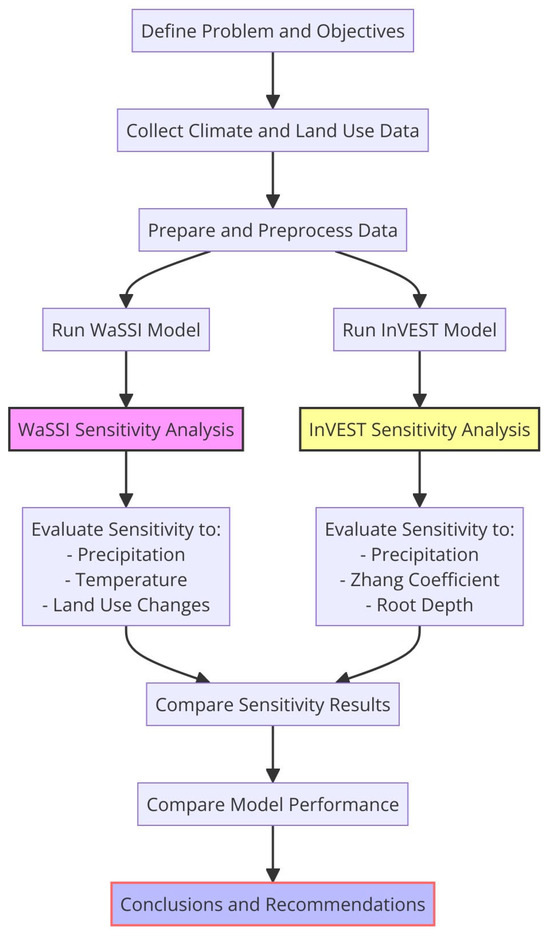
Figure 1.
Comparative analysis steps for WaSSI and InVEST models in water yield estimation.
2. Methods and Materials
2.1. Methods
2.1.1. Water Yield Module (WaSSI)
The Water Supply Stress Index (WaSSI) model defines water yield as the streamflow exiting a watershed after accounting for losses due to soil water storage changes, evaporation, and transpiration. This metric is calculated in millimeters per year and considers variations in land use and cover. The WaSSI model was developed by the USDA Forest Service Southern Research Station and has undergone extensive validation and comparison against other hydrological models [6,14,15,30,31,32,33]. Its design allows for analyses at both annual and monthly scales, focusing on responses under wet and dry conditions.
The WaSSI employs a temperature-driven conceptual model to separate precipitation into rain and snow [34]. The model computes monthly metrics such as infiltration, surface runoff, soil moisture, and baseflow for each land use type in a watershed using the Sacramento Soil Moisture Accounting Model (SAC-SMA) algorithms [35,36]. The soil profile is modeled as two layers—a shallow upper layer and a deeper lower layer—each containing tension water storage and free water storage components. These interact to produce surface runoff, interflow, percolation, and baseflow.
Monthly evapotranspiration (ET) is calculated using potential ET [37], precipitation, and leaf area index (LAI) based on empirical data derived from eddy covariance measurements [14]. For impervious surfaces, storage and ET are considered negligible, and all precipitation is assumed to contribute directly to runoff. Although this assumption may lead to overestimation in certain regions, it is necessary given uncertainties about water storage and connectivity on impervious surfaces at a regional scale.
Water yield for each land use type within a watershed is calculated as the sum of surface runoff, interflow, and baseflow, adjusted for soil storage changes, evaporation, and transpiration losses. These calculations are aggregated into area-weighted averages across different land use types and expressed in millimeters per year. The model then routes the water yield downstream through the river network, accumulating contributions from upstream watersheds to determine the surface water supply at watershed outlets, expressed in cubic meters per year. Figure 2 illustrates the hydrologic processes and land cover classes simulated by the WaSSI model, including key variables such as precipitation (P), evapotranspiration (ET), streamflow (Q), and changes in water storage (ΔS) [15,38]. All terms are expressed in water depth units (e.g., millimeters). The function f incorporates vegetation (via LAI) and meteorological drivers (PET and P) to calculate actual evapotranspiration. This approach ensures that the model captures the interaction between vegetation and water availability effectively.
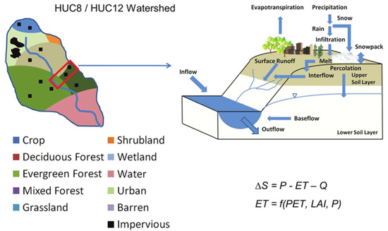
Figure 2.
Land cover classes and hydrologic processes simulated by the WaSSI: ΔS = change in surface and groundwater storage; Q = streamflow or water yield; ET = evapotranspiration; PET: potential evapotranspiration; P = precipitation, and LAI = leaf area index [15].
2.1.2. Water Yield Module (InVEST)
The water yield model that quantifies the average yearly runoff, denoted as water yield in millimeters, across the watershed is shown in Figure 3. In this study, the workflow of the InVEST model, as shown in Figure 3, was applied to the study area using available data. Inputs such as precipitation, temperature, and land use/land cover (LULC) were processed alongside parameters like plant-available water content and the Zhang parameter (Z) to calculate annual evapotranspiration and water yield. The model was evaluated using sensitivity analysis, time-series calibration (1987–1991), and validation (1991–2020), ensuring accuracy and reliability based on the existing datasets.
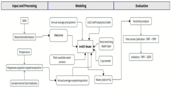
Figure 3.
A view of InVEST water yield model.
The InVEST model was applied to estimate the annual water yield (equation) for a single sub-watershed using available datasets. Water yield represents the portion of precipitation (P) that contributes to runoff after accounting for evapotranspiration (AETJ) losses. The model is based on the following equation:
Here, AETJ is calculated using Zhang curve, which integrates precipitation (P), potential evapotranspiration PETj, and the Zhang parameter (Z), as follows:
The parameter ω, which adjusts for soil water retention and hydrogeological conditions, is defined as the following:
In these equations, the following are used:
P: annual precipitation (mm/year), derived from PRISM climate data.
PETj: potential evapotranspiration (mm/year) for each land use type j, calculated using climatic and vegetation data.
AWC: plant-available water capacity of the soil, obtained from global soil databases.
Z: empirical constant representing local precipitation patterns and hydrogeological conditions.
The InVEST model assumes that all precipitation not lost to evapotranspiration contributes to runoff, leaving the sub-watershed as water yield. The Zhang curve effectively captures the interplay between vegetation characteristics, soil water retention, and climatic conditions, providing a robust representation of annual water yield dynamics. To ensure reproducibility, all equations, parameters, and data sources are explicitly provided, and the methodology builds upon reliable datasets, including PRISM climate data and global soil databases. By integrating precipitation, evapotranspiration, soil properties, and vegetation characteristics, the InVEST model outputs are transparent and reproducible, making them highly applicable for watershed management and planning in the study area.
2.2. Materials
2.2.1. Model Input Data
We leveraged an extensive and varied set of input data to operationalize the WaSSI and InVEST models. Table 1 and Table 2 summarize the data sources used by the WaSSI and InVEST models, respectively, for estimating water yield in the Croatan National Forest, highlighting key input parameters such as precipitation, land use/land cover data, and soil characteristics essential for modeling. These tables provide useful insights into the data inputs and processing procedures crucial for water yield estimation in the study area. Standardizing the spatial resolution to a uniform 30 m for both the WaSSI and InVEST models is important, as this step is foundational in ensuring the integrity and compatibility of data within the analysis process and ensures that analyses are based on data of similar quality and accuracy, thus making comparative analyses between models more precise and valid. Both models rely on precise spatial and computational analyses that require input data of a specific resolution and accuracy to deliver reliable predictions and outcomes. Also, the datasets were converted to the North American Datum 1983 (NAD 83) UTM Zone 17N for input into the InVEST model [39].

Table 1.
Data sources for the WaSSI model.
Table 2.
The used data characteristics for the InVEST Model.
Figure 4, Figure 5, Figure 6, Figure 7 and Figure 8 depict the layers obtained for land use, reference evapotranspiration, crop coefficient (kc), plant-available water capacity (PAWC), preparation, and root depth restriction. These layers are utilized as inputs for the InVEST model to calculate water yield. The physical quantities depicted in Figure 4, Figure 5, Figure 6, Figure 7 and Figure 8, including land use/land cover, precipitation, potential evapotranspiration, and soil characteristics, are derived from high-resolution raster datasets with a pixel size of approximately 100 m.
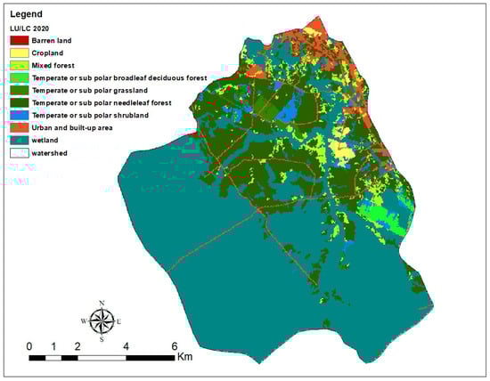
Figure 4.
Different LU/LC.
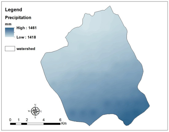
Figure 5.
Annual precipitation (mm).
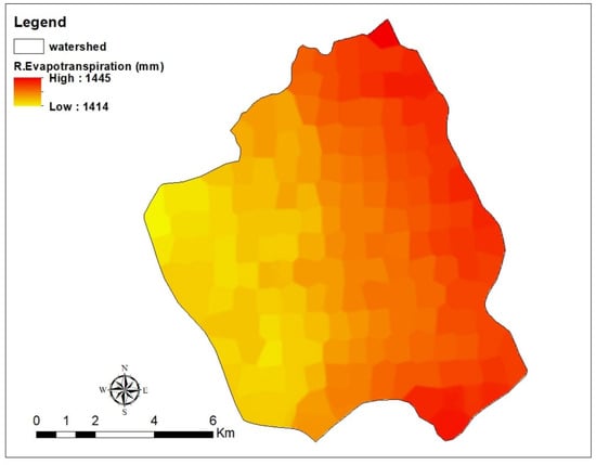
Figure 6.
Reference evapotranspiration (raster layer) (mm).
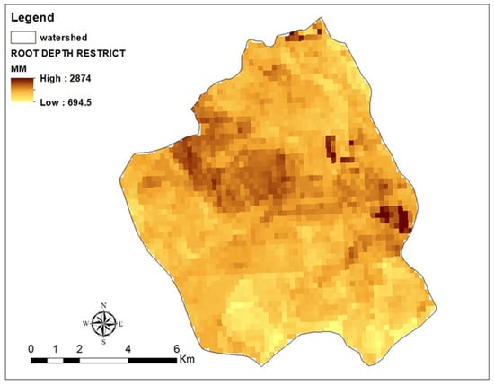
Figure 7.
Root depth restriction (raster layer) (mm).
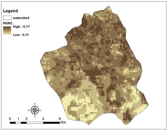
Figure 8.
Plant-available water content (raster layer) (%).
2.2.2. Study Area
The Croatan National Forest, located in the coastal plain region of North Carolina, USA, presents a unique case study due to its diverse ecosystems and strategic geographical setting. Encompassing approximately 647 km2, the forest is bordered by the Bogue Sound, the White Oak River, and the Neuse River (Figure 9). This position creates a unique interplay between terrestrial and aquatic ecosystems, supporting a rich biodiversity within its saltwater estuaries, pocosins (elevated swamps), and pine forests. The area is characterized by low elevation, generally ranging from sea level to slightly over 9 m above sea level [46]. The United States Geological Survey (USGS) gauge station 0209257120, located at W.P. Brice Creek below SR1101 near Riverdale, NC, was selected as the nearest and most representative hydrological station to the study area [47]. This station, with a drainage area of approximately 29 km2 and classified under the Hydrologic Unit Code (HUC) 03020204, provided observed data from 1987 to 1991. Although covering only 5 years, this dataset is useful for comparing observed water yields with those predicted by the InVEST and WaSSI models, helping to evaluate differences and model performance in the study area.
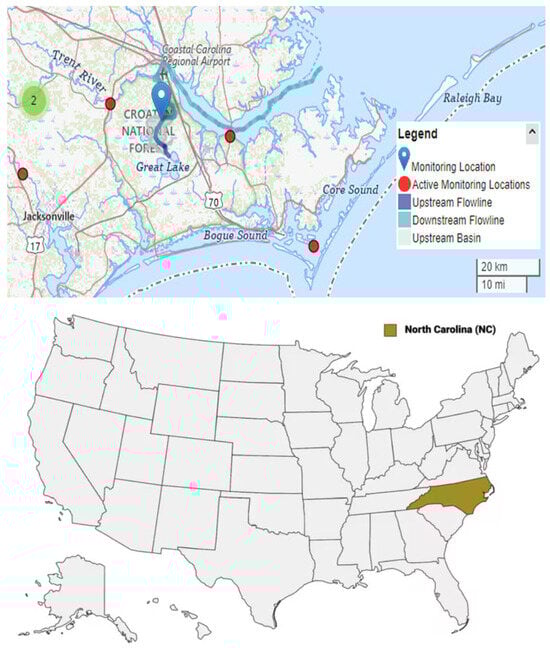
Figure 9.
The area in the upper map represents the Croatan National Forestand the hydrology station, and the lower highlights North Carolina in red, where the Croatan National Forest is in its coastal region.
3. Results
In this section, the results of the study are presented, focusing exclusively on water yield, as derived from the application of the WaSSI and InVEST models. The analysis highlights the key outputs related to water yield predictions and their sensitivity to variations in input parameters, such as precipitation and land use. The findings provide a clearer understanding of how different factors influence water yield in the study area.
3.1. Sensitivity Analysis
3.1.1. Sensitivity Analysis of the WaSSI Model
To conduct a comprehensive sensitivity analysis using the WaSSI model, we examined the effects of a 10% increase in both precipitation and temperature on water yield. The 10% increment was chosen as a representative value to balance computational efficiency with meaningful insight into the model’s behavior. While more increments could provide a finer understanding of sensitivity, this approach aimed to focus on capturing key trends.
The analysis revealed that a 10% increase in precipitation leads to a 21.14% increase in water yield, indicating the high sensitivity of the model to precipitation changes with a calculated sensitivity of 2.114. This implies that each 1% increase in precipitation leads to a 2.114% increase in water yield, underscoring the significant influence of precipitation on the model’s hydrological outputs. Conversely, the sensitivity analysis to temperature changes demonstrated that a 10% increase in temperature results in a 5.27% decrease in water yield, with a calculated sensitivity of −0.527. Therefore, each 1% increase in temperature corresponds to a 0.527% decrease in water yield, highlighting the model’s sensitivity to temperature variations. These findings collectively underscore the critical impact of climatic parameters on the hydrological responses simulated by the WaSSI model, providing valuable insights for understanding and predicting the effects of climate variability on water resources. Additionally, the sensitivity analysis of the WaSSI model to changes in forest land cover fraction indicates that a 10% decrease in forest land cover results in a 0.225% decrease in water yield, with a calculated sensitivity of 0.0225. This shows that each 1% decrease in forest land cover leads to a 0.0225% decrease in water yield. Furthermore, the sensitivity analysis of the WaSSI model to changes in forest LAI indicates that a 10% decrease in LAI results in a 1.06% increase in water yield, with a calculated sensitivity of −0.106. Conversely, a 10% increase in LAI results in a 0.97% decrease in water yield, with a calculated sensitivity of −0.097. The model shows very low sensitivity to changes in land cover and LAI changes. Figure 10 illustrates the sensitivity of the WaSSI model to key parameters affecting water yield.
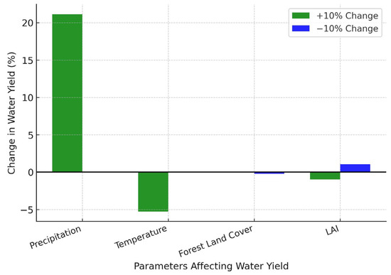
Figure 10.
Sensitivity of the WaSSI model to key parameters for water yield.
Finally, the WaSSI model was evaluated for predicting observed values from 1987 to 1991. Using polynomial regression (degree 2) and cross-validation, the model achieved a Mean Absolute Error (MAE) of 8.68 and a Root Mean Square Error (RMSE) of 10.38. The model’s accuracy, with a Mean Absolute Percentage Error (MAPE) of 12.83%, reached 87.17%, indicating significant prediction accuracy.
Additionally, the Nash–Sutcliffe Efficiency (NSE), a widely used statistical measure for evaluating the predictive performance of hydrological models, was calculated to be 0.935. The NSE formula is expressed as:
Here, MSE is the Mean Squared Error between observed and predicted data. An NSE value of 1 indicates perfect predictive performance, while values close to 0 or negative suggest poor agreement between predictions and observations. In this study, the WaSSI model demonstrated excellent performance for water yield prediction with an NSE of approximately 0.935, indicating a strong agreement between observed and predicted values.
3.1.2. Sensitivity Analysis of the InVEST Model
In a sensitivity analysis, the InVEST–AWY model exhibited low sensitivity to the Zhang coefficient, as shown in a study [48]. Also, based on the findings of the study, the Kc value demonstrates minimal sensitivity in influencing water yield values within the InVEST-AWY [49]. However, our research conducted on the Croatan National Forest, a coastal forest in North Carolina, underscored the critical importance of selecting suitable model parameters and input data. Notably, precipitation was identified as having a significant influence on water yield outcomes, as highlighted in the findings of this study. A 10% increase in precipitation resulted in 26% increase in water yield, while in some catchments, a 10% increase in reference evapotranspiration and a 14% decrease in water yield. Increasing the root depth restriction and plant-available water content (PAWC) had little effect on yield, with a 10% increase in root depth and PAWC resulting in only a negligible 0.2–0.3% increase in water yield. The sensitivity analysis results factor affecting water yield in the InVEST model illustrated in Figure 11.
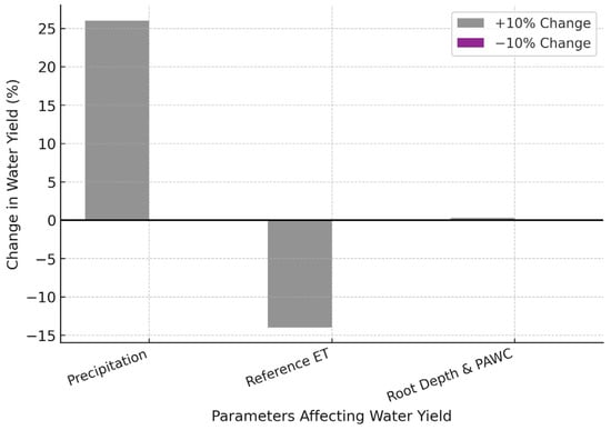
Figure 11.
Sensitivity analysis of key parameters affecting water yield in the InVEST model.
Model Sensitivity to Z and Kc
Following a study, the Zhang coefficient Z can be estimated using the formula Z = 0.2 × N, where N represents the number of rainfall events per year [50]. The annual number of rainy days in North Carolina is reported to be 130, according to current results (n.d.). Consequently, N is equal to 130, resulting in a Z value of 26. As Z values range from 1 to 30, we used this Z value range to evaluate the change in water yield. Figure 10 illustrates the sensitivity of mean water yield (WY-mn) to variations in Z values, which showed a consistent decrease in water yield as Z increases, indicating a strong negative correlation. This decline is particularly pronounced at lower values of Z (from 1 to approximately 10), demonstrating the model’s high sensitivity to changes within this range. As Z further increases, the rate of decrease in water yield gradually becomes more moderate and remains relatively stable, suggesting lesser impacts of changes at higher values of Z. This sensitivity analysis underscores the importance of the Zhang coefficient as a crucial parameter affecting water yield, especially at lower values.
Figure 12 illustrates the variation in water yield (WY) as a function of different Zhang coefficient (Z) values, highlighting the model’s sensitivity to changes in this parameter.
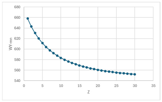
Figure 12.
Variation in water yield (WY) based on different Zhang coefficients (Z).
In contrast, the results of the sensitivity analysis indicated that increasing Kc values in crops by 30% would lead to a decrease in water yield by 11.3%, whereas a 30% reduction in Kc values would result in a 2.4% increase in water yield. These findings suggest that the Kc value does not significantly influence the InVEST–AWY model’s sensitivity, unlike the Z parameter. These findings suggest that the Kc value has a relatively minor influence on the InVEST–AWY model’s sensitivity compared to the Z parameter. While Kc plays a role in modifying water yield outcomes, the significant impact of the Z parameter highlights its dominant role in determining the model’s sensitivity, particularly in the context of water resource management in coastal forests.
3.1.3. Calibration
In this study, the InVEST model was calibrated to assess annual water yield in the Croatan National Forest area. This calibration was based on parameter Z, which indicates the temporal distribution of rainfall throughout the year. In this study, the InVEST model was calibrated to assess annual water yield in the Croatan National Forest area. This calibration was based on parameter Z, which indicates the temporal distribution of rainfall throughout the year [51]. Initially, daily rainfall data was collected from reliable climatic sources, specifically from the PRISM Climate Group database at Oregon State University, which provides high-resolution precipitation records for the Croatan National Forest area [40]. These data were used as input for the InVEST–AWY model to simulate water yield outcomes accurately. During the sensitivity analysis, it was concluded that Z should be derived from the number of rainy days using this formula, resulting in a Z value of 26. The available hydrological station data for the study area included only 5 years of records, which was insufficient for direct calibration based solely on climatic data. However, these data were valuable for validating the model outputs and assessing its accuracy. To address the limitation, parameter Z, derived from annual rainfall events, was used to calibrate the model as a practical alternative, ensuring robust results under data-limited conditions.
After determining the Z value, the InVEST model was run and the model outputs of water yield were compared with the actual basin yield data observed from the above-mentioned hydrological station over the 5-year period to evaluate the model’s accuracy. The model exhibited a Mean Absolute Error (MAE) of 21.02 and a Mean Squared Error (MSE) of 653.18, resulting in a Root Mean Squared Error (RMSE) of 25.56. Additionally, the Mean Absolute Percentage Error (MAPE) of the model is 29.29%. In hydrological studies, the acceptable error level depends on the type of application and the accuracy of the available data. Commonly, metrics such as the coefficient of determination (R2), Nash–Sutcliffe Efficiency (NSE), and percentage relative error are employed to evaluate model performance [52]. According to the literature, an accuracy rate above 70% is generally considered acceptable for many streamflow prediction models in operational and management contexts [53]. In this study, the model achieved an accuracy rate of 70.71%, which falls within the acceptable range for similar models. Additionally, the InVEST model achieved an NSE of approximately 0.924, indicating reliable performance in predicting water yield. However, improving the model’s accuracy through optimization of input data and modeling parameters could be explored in future research.
Finally, to compare the predictive performance of the WaSSI and InVEST models, Figure 13 presents their respective prediction errors in estimating water yield. This comparison highlights the differences in model accuracy and facilitates a better assessment of their reliability.
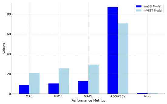
Figure 13.
Comparison of water yield prediction performance between the WaSSI and InVEST models based on key evaluation metrics.
4. Discussion
Comparing WaSSI and InVEST models for water yield prediction in the Croatan coastal forest really underscores how important it is to choose the right tools based on the specific ecological context and the data you have on hand. Both models come with their own set of strengths and weaknesses, and how they perform can vary quite a bit depending on things like the scale of the analysis, how much data are available, and the level of accuracy needed for simulations. Below, we dive into how these two models stack up, based on what this study has shown. These findings highlight the importance of further exploring the capabilities of both models under varying data conditions to enhance their applicability for diverse hydrological assessments. It is recommended that future studies examine and compare carbon storage between the two models, particularly the WaSSI, in coastal areas. Coastal regions, due to their high sensitivity to climate change and the critical role of carbon storage in reducing greenhouse gases, require a precise evaluation of related ecosystem services. This comparison can help identify the strengths and weaknesses of the models in assessing and managing these essential services.
4.1. Performance and Sensitivity
Both models show an acceptable margin of error when it comes to hydrological predictions, but their performance and sensitivity differ in keyways—especially when factoring in climate and land use changes:
- The WaSSI is more accurate than the InVEST. Its metrics—a Mean Absolute Error (MAE) of 8.68, a Root Mean Square Error (RMSE) of 10.38, and a Mean Absolute Percentage Error (MAPE) of 12.83%—are also paired with an accuracy rate of 87.17%. The WaSSI really has acceptable results in situations where there are not much data to work with. It is also highly sensitive to changes in precipitation. For instance, if precipitation increases by 10%, water yield jumps by 21.14%, making this model an excellent fit for studies on how climate changes might play out.
- The InVEST, on the other hand, is not as precise, with an MAE of 21.02, an RMSE of 25.56, an MAPE of 29.29%, and an accuracy rate of 70.71%. But it has advantages. The InVEST is highly sensitive to land use changes, especially when dealing with parameters like Zhang’s coefficient. This makes it a tool for detailed, localized studies—if there are high-resolution input data to work with.
To ensure greater confidence in model accuracy, both the WaSSI (NSE ≈ 0.935) and InVEST (NSE ≈ 0.924) demonstrate strong performance based on NSE values exceeding 0.9, which are considered excellent in hydrological modeling [54]. However, the WaSSI performs slightly better due to lower error metrics, making it more reliable for general water yield predictions, especially under data-scarce conditions. The InVEST, while slightly less precise, remains suitable for detailed studies requiring sensitivity to land use changes. While both models exhibit strong hydrological prediction capabilities, their performance differs significantly in terms of error margins and sensitivity to key parameters. The WaSSI demonstrates lower prediction errors, making it a more reliable model for estimating water yield, especially in data-scarce conditions. However, it is predominantly influenced by climatic variables, particularly precipitation, while showing limited sensitivity to land use changes. In contrast, the InVEST, despite its higher error margins, responds more dynamically to land use variations, particularly changes in the Zhang coefficient. This makes it a valuable tool for assessing the impacts of land use modifications on hydrological processes. Ultimately, the trade-off between higher predictive accuracy versus greater sensitivity to land use parameters determines the optimal model choice based on the study’s specific objectives.
4.2. Applications of the WaSSI and InVEST
Past research gives us some great insights into how these models perform in different scenarios:
- The WaSSI has been successfully applied in a wide range of environments.
- For instance, a study found that in arid and semi-arid areas like Rwanda, the WaSSI had better accuracy for simulating water yield in watersheds, even when the available data were limited. And of course, the InVEST performed well under the sub-watershed [55].
- Similarly, a study tested the WaSSI in the Pearl River Basin, which has a mix of hydrological and coastal systems. It turned out to be effective for modeling water-carbon interactions [56].
Our findings and these results show that the WaSSI is reliable in many settings, from semi-arid landscapes to coastal regions, even when data are sparse. That said, when it comes to the Croatan coastal forest, the study had to rely on historical data from 1987 to 1991 since there are not any active hydrological stations in the area. This limitation made it hard to directly compare observed and simulated data.
4.3. Suggestions for Future Research
Here are a few ideas for how future work can use these models effectively:
- Better DataIn areas without active hydrological stations, creating synthetic datasets using virtual simulations by creating virtual stations could make a big difference. Combining satellite data, climate models, and even AI to reconstruct water flow data could help fill in the gaps.
- Long-Term ImpactsLooking at how climate change and land use shifts affect water resources in coastal forests over time is critical. Since the WaSSI responds so well to environmental changes, it could be especially useful for these kinds of studies.
- Comparison of Other Model ModulesComparing WaSSI and InVEST models for carbon storage in coastal areas could highlight their strengths and weaknesses, aiding in the evaluation and management of essential ecosystem services.
- Model ComparisonsFuture studies should compare the WaSSI and InVEST with traditional models like SWAT and VIC to enhance our understanding of water resource management in diverse ecosystems.
5. Conclusions
This study, in addition to confirming previous findings, highlights the scarcity of hydrological data, the lack of sufficient hydrological stations, and the need for advanced modeling in coastal areas such as Croatan. The success of the WaSSI model in diverse conditions, including semi-arid and coastal regions, not only validates the results of this research but also underscores the significant potential of this model for use in long-term sustainable water resource planning by managers. Considering climate change and the need for long-term predictions., the adoption of innovative methods, the development of reliable datasets, and the integration of models can be essential for enhancing ecosystem resource management. This study demonstrated that the WaSSI model, due to its simplicity and processing speed, performs better for large-scale predictions and in data-scarce regions, whereas the InVEST model, with its more complex design, requires high-quality data for more detailed studies. Ultimately, the findings of this research represent an important step in evaluating hydrological models in coastal ecosystems and can serve as a valuable foundation for future research in this field.
Author Contributions
All research work, including conceptualization, methodology, software, formal analysis, investigation, resources, data curation, original draft writing, visualization, and other research processes, was independently conducted by M.F. The remaining authors (S.A.C.N., S.B., P.V.C. and J.P.R.) contributed to writing—review and editing. All authors have read and agreed to the published version of the manuscript.
Funding
This research received no external funding.
Data Availability Statement
The original contributions presented in this study are included in the article. Further inquiries can be directed to the corresponding author.
Acknowledgments
The authors would like to thank all contributors to this research for their valuable input and support.
Conflicts of Interest
The authors declare no conflicts of interest.
Disclaimer
Any opinions, findings, conclusions, or recommendations expressed in this material are those of the authors and do not necessarily reflect the views of the USDA. Any use of trade, firm, or product names is for descriptive purposes only and does not imply endorsement by the U.S. Government.
References
- Parida, B.R.; Pandey, A.C.; Behera, M.D.; Kumar, N. Handbook of Himalayan Ecosystems and Sustainability: Spatio-Temporal Monitoring of Water Resources and Climate; CRC Press: Boca Raton, FL, USA, 2022. [Google Scholar]
- Tzanakakis, V.A.; Capodaglio, A.G.; Angelakis, A.N. Insights into global water reuse opportunities. Sustainability 2023, 15, 13007. [Google Scholar] [CrossRef]
- Wu, H.; Yang, C.; Xie, C.; Man, Z.; He, S.; Qin, Y.; Che, S. Quantification of contribution of climate change and land use change on urban ecosystem service using multi-scale approach. Ecol. Indic. 2024, 167, 112619. [Google Scholar] [CrossRef]
- Qin, H.; Cai, X.; Zheng, C. Water demand predictions for megacities: System dynamics modeling and implications. Water Policy 2018, 20, 53–72. [Google Scholar] [CrossRef]
- Sannigrahi, S.; Zhang, Q.; Joshi, P.K.; Sutton, P.C.; Keesstra, S.; Ray, P.S.; Pilla, F.; Basu, B.; Wang, Y.; Jha, S.; et al. Examining effects of climate change and land use dynamics on biophysical and economic values of ecosystem services in a natural reserve region. J. Clean. Prod. 2020, 256, 120346. [Google Scholar] [CrossRef]
- Caldwell, P.V.; Kennen, J.G.; Sun, G.; Kiang, J.E.; Butcher, J.B.; Eddy, M.C.; Hay, L.E.; LaFontaine, J.H.; Hain, E.F.; Nelson, S.A.C.; et al. A comparison of hydrologic models for ecological flows and water availability. Ecohydrology 2015, 8, 1525–1546. [Google Scholar] [CrossRef]
- Li, M.; Liang, D.; Xia, J.; Song, J.; Cheng, D.; Wu, J.; Cao, Y.; Sun, H.; Li, Q. Evaluation of water conservation function of Danjiang River Basin in Qinling Mountains, China based on InVEST model. J. Environ. Manag. 2021, 286, 112212. [Google Scholar] [CrossRef]
- Wu, Y.; Zhang, X.; Li, C.; Xu, Y.; Hao, F.; Yin, G. Ecosystem service trade-offs and synergies under influence of climate and cover change in an afforested semiarid basin, China. Ecol. Eng. 2020, 159, 106083. [Google Scholar] [CrossRef]
- Van der Biest, K.; Vrebos, D.; Staes, J.; Boerema, A.; Bodí, M.B.; Fransen, E.; Meire, P. Evaluation of the accuracy of land-use based ecosystem service assessments for different thematic resolutions. J. Environ. Manag. 2015, 156, 41–51. [Google Scholar] [CrossRef]
- Tang, L.L.; Cai, X.B.; Gong, W.S.; Lu, J.Z.; Chen, X.L.; Lei, Q.; Yu, G.L. Increased vegetation greenness aggravates water conflicts during lasting and intensifying drought in the Poyang Lake watershed, China. Forests 2018, 9, 24. [Google Scholar] [CrossRef]
- De Koning, J.; Turnhout, E.; Winkel, G.; Blondet, M.; Borras, L.; Ferranti, F.; Geitzenauer, M.; Sotirov, M.; Jump, A. Managing climate change in conservation practice: An exploration of the science–management interface in beech forest management. Biodivers. Conserv. 2014, 23, 3647–3671. [Google Scholar] [CrossRef]
- Peng, J.; Hu, X.; Wang, X.; Meersmans, J.; Liu, Y.; Qiu, S. Simulating the impact of the Grain-for-Green Programme on ecosystem services trade-offs in Northwestern Yunnan, China. Ecosyst. Serv. 2019, 39, 100981. [Google Scholar] [CrossRef]
- Sun, S.; Sun, G.; Cohen Mack, E.; McNulty, S.; Caldwell, P.; Duan, K.; Zhang, Y. Predicting future US water yield and ecosystem productivity by linking an ecohydrological model to WRF dynamically downscaled climate projections. Hydrol. Earth Syst. Sci. Discuss. 2015, 12, 12703–12747. [Google Scholar]
- Guo, Q.; Yu, C.; Xu, Z.; Yang, Y.; Wang, X. Impacts of climate and land-use changes on water yields: Similarities and differences among typical watersheds distributed throughout China. J. Hydrol. Reg. Stud. 2023, 45, 101294. [Google Scholar] [CrossRef]
- Caldwell, P.V.; Sun, G.; McNulty, S.G.; Cohen, E.C.; Moore Myers, J.A. Impacts of impervious cover, water withdrawals, and climate change on river flows in the conterminous US. Hydrol. Earth Syst. Sci. 2012, 16, 2839–2857. [Google Scholar] [CrossRef]
- Sabater, S.; Bregoli, F.; Acuña, V.; Barceló, D.; Elosegi, A.; Ginebreda, A.; Marcé, R.; Muñoz, I.; Sabater-Liesa, L.; Ferreira, V. Effects of human-driven water stress on river ecosystems: A meta-analysis. Sci. Rep. 2018, 8, 11462. [Google Scholar] [CrossRef]
- Xu, C.; Jiang, Y.; Su, Z.; Liu, Y.; Lyu, J. Assessing the impacts of the Grain-for-Green Programme on ecosystem services in the Jinghe River Basin, China. Ecol. Indic. 2022, 137, 108757. [Google Scholar] [CrossRef]
- Belay, T.; Melese, T.; Senamaw, A. Impacts of land use and land cover change on ecosystem service values in the Afroalpine area of Guna Mountain, Northwest Ethiopia. Heliyon 2022, 8, e12246. [Google Scholar] [CrossRef]
- Johnson, J.A.; Baldos, U.L.; Corong, E.; Thakrar, S. Investing in nature can improve equity and economic returns. Proc. Natl. Acad. Sci. USA 2023, 120, e2220401120. [Google Scholar] [CrossRef]
- Yu, J.; Yuan, Y.; Nie, Y.; Ma, E.; Li, H.; Geng, X. Temporal-spatial analysis of water yield evolution in Dali County. Sustainability 2015, 7, 6069–6085. [Google Scholar] [CrossRef]
- Aghsaei, H.; Dinan, N.M.; Moridi, A.; Asadolahi, Z.; Delavar, M.; Fohrer, N.; Wagner, P.D. Effects of dynamic land use/land cover change on water resources and sediment yield in the Anzali wetland catchment, Gilan, Iran. Sci. Total Environ. 2020, 712, 136449. [Google Scholar] [CrossRef]
- Hamel, P.; Chaplin-Kramer, R.; Sim, S.; Mueller, C. A new approach to modeling the sediment retention service (InVEST 3.0): Case study of the Cape Fear catchment, North Carolina, USA. Sci. Total Environ. 2015, 524–525, 166–177. [Google Scholar] [CrossRef]
- Sharps, K.; Masante, D.; Thomas, A.; Jackson, B.; Redhead, J.; May, L.; Prosser, H.; Cosby, B.; Emmett, B.; Jones, L. Comparing strengths and weaknesses of three ecosystem services modelling tools in a diverse UK river catchment. Sci. Total Environ. 2017, 584–585, 118–130. [Google Scholar] [CrossRef]
- Agudelo, C.A.R.; Hurtado Bustos, S.L.; Moreno, C. Modeling interactions among multiple ecosystem services: A critical review. Ecol. Model. 2020, 429, 109103. [Google Scholar] [CrossRef]
- Arnold, J.G.; Srinivasan, R.; Muttiah, R.S.; Williams, J.R. Large area hydrologic modeling and assessment part I: Model development. J. Am. Water Resour. Assoc. 1998, 34, 73–89. [Google Scholar] [CrossRef]
- Liang, X.; Lettenmaier, D.P.; Wood, E.F.; Burges, S.J. A simple hydrologically based model of land surface water and energy fluxes for general circulation models. J. Geophys. Res. Atmos. 1994, 99, 14415–14428. [Google Scholar] [CrossRef]
- Ury, E.A.; Yang, X.; Wright, J.; Bernhardt, E. Rapid deforestation of a coastal landscape driven by sea level rise and extreme events. Ecol. Appl. 2021, 31, e2339. [Google Scholar] [CrossRef]
- Dennedy-Frank, P.; Muenich, R.; Chaubey, I.; Ziv, G. Comparing two tools for ecosystem service assessments regarding water resources decisions. J. Environ. Manag. 2016, 177, 331–340. [Google Scholar] [CrossRef]
- Panigrahi, B.; Goyal, M.R. Modeling Methods and Practices in Soil and Water Engineering; CRC Press: Boca Raton, FL, USA, 2017. [Google Scholar]
- Caldwell, P.V.; Sun, G.; Cohen, E.; McNulty, S.G.; Hallema, D.W.; Nyman, P. Impacts of drought-related wildfires on hydrological processes and water quality in the southern Appalachian Mountains. Hydro. Process. 2020, 34, 2368–2383. [Google Scholar]
- Li, C.; Sun, G.; Caldwell, P.V.; Cohen, E.; Fang, Y.; Zhang, Y.; Oudin, L.; Sanchez, G.M.; Meentemeyer, R.K. Impacts of urbanization on watershed water balances across the conterminous United States. Water Resour. Res. 2020, 56, e2019WR026574. [Google Scholar] [CrossRef]
- Schwalm, C.R.; Huntzinger, D.N.; Fisher, J.B.; Michalak, A.M.; Bowman, K.; Ciais, P.; Cook, R.; El-Masri, B.; Hayes, D.; Huang, M.; et al. Toward “optimal” integration of terrestrial biosphere models. Geophys. Res. Lett. 2015, 42, 4418–4428. [Google Scholar] [CrossRef]
- Sun, G.; Caldwell, P.V.; McNulty, S.G. Modelling the potential role of forest thinning in maintaining water supplies under a changing climate across the conterminous United States. Hydrol. Process. 2015, 29, 5016–5030. [Google Scholar] [CrossRef]
- Wolock, D.M.; McCabe, G.J. Estimates of runoff using water-balance and atmospheric general circulation models. J. Am. Water Resour. Assoc. 1999, 35, 1341–1350. [Google Scholar] [CrossRef]
- Burnash, R.J.C.; Ferral, R.L.; McGuire, R.A. A Generalized Streamflow Simulation System: Conceptual Modeling for Digital Computers; U.S. Department of Commerce, National Weather Service: Silver Spring, MD, USA, 1973. [Google Scholar]
- Burnash, R.J.C.; Singh, V.P. The Sacramento Soil Moisture Accounting Model (SAC-SMA). In Computer Models of Watershed Hydrology; Water Resources Publications: Littleton, CO, USA, 1995; pp. 443–476. [Google Scholar]
- Hamon, W.R. Computation of direct runoff amounts using meteorological data. J. Appl. Meteorol. 1963, 2, 680–682. [Google Scholar]
- Shao, R.; Zhang, B.; He, X.; Su, T.; Li, Y.; Long, B.; Wang, X.; Yang, W.; He, C. Historical water storage changes over China’s Loess Plateau. Water Resour. Res. 2021, 57, e2020WR02866. [Google Scholar] [CrossRef]
- U.S. Geological Survey (USGS). Available online: https://pubs.usgs.gov (accessed on 31 August 2023).
- PRISM Climate Group, Oregon State University. High-Resolution Precipitation Records for the Croatan National Forest Area. 2022. Available online: http://prism.oregonstate.edu (accessed on 31 August 2023).
- NASA. MODIS Land Cover Type Product (MCD12Q1). Available online: https://modis.gsfc.nasa.gov/data/dataprod/mod12.php (accessed on 31 August 2023).
- United States Department of Agriculture (USDA). Available online: https://www.usda.gov (accessed on 31 August 2023).
- Sun, G.; Domec, J.-C.; Amatya, D.M. Forest hydrology processes and water resource management in a changing environment. In Forest Hydrology: Processes, Management, and Assessment; Amatya, D.M., Williams, T.M., Bren, L., de Jong, C., Eds.; USDA Forest Service: Washington, DC, USA, 2016; pp. 32–50. [Google Scholar]
- FAO. Harmonized World Soil Database; Version 1.0; Food and Agriculture Organization of the United Nations: Rome, Italy, 1998; Available online: https://www.fao.org/soils-portal (accessed on 31 August 2023).
- U.S. Geological Survey. National Land Cover Database (NLCD). Available online: https://www.usgs.gov/centers/eros/science/national-land-cover-database (accessed on 31 August 2023).
- Moonier, H. Predictive Occurrence Modeling for Three Rare Plants Within the Croatan National Forest. Master’s Thesis, North Carolina State University, Raleigh, NC, USA, 2023. [Google Scholar]
- USGS. Water Data; U.S. Geological Survey: Reston, VA, USA. Available online: https://waterdata.usgs.gov/nwis (accessed on 31 August 2023).
- Redhead, J.W.; Stratford, C.; Sharps, K.; Jones, L.; Ziv, G.; Clarke, D.; Oliver, T.H.; Bullock, J.M. Empirical validation of the InVEST water yield ecosystem service model at a national scale. Sci. Total Environ. 2016, 569–570, 1418–1426. [Google Scholar] [CrossRef]
- Valencia, J.; Guryanov, V.V.; Mesa-Diez, J.; Tapasco, J.; Gusarov, A.V. Assessing the effectiveness of the use of the InVEST annual water yield model for the rivers of Colombia: A case study of the Meta River Basin. Water 2023, 15, 1617. [Google Scholar] [CrossRef]
- Donohue, R.J.; Roderick, M.L.; McVicar, T.R.; Farquhar, G.D. Influence of Vegetation on the Hydrological Cycle: Insights from a Global Budyko Analysis. Water Resour. Res. 2012, 48, W07503. [Google Scholar]
- Hamel, P.; Guswa, A.J. Uncertainty analysis of a spatially explicit annual water-balance model: Case study of the Cape Fear basin, North Carolina. Hydrol. Earth Syst. Sci. 2015, 19, 839–853. [Google Scholar] [CrossRef]
- Nash, J.E.; Sutcliffe, J.V. River flow forecasting through conceptual models. J. Hydrol. 1970, 10, 282–290. [Google Scholar]
- Moriasi, D.N.; Arnold, J.G.; Van Liew, M.W.; Bingner, R.L.; Harmel, R.D.; Veith, T.L. Model evaluation guidelines for systematic quantification of accuracy in watershed simulations. Trans. ASABE. 2007, 50, 885–900. [Google Scholar] [CrossRef]
- Duc, L.; Sawada, Y. A signal-processing-based interpretation of the Nash–Sutcliffe efficiency. Hydrol. Earth Syst. Sci. 2023, 27, 1827–1839. [Google Scholar] [CrossRef]
- Bagstad, K.J.; Cohen, E.; Ancona, Z.H.; McNulty, S.G.; Sun, G. The sensitivity of ecosystem service models to choices of input data and spatial resolution. Appl. Geogr. 2018, 93, 25–36. [Google Scholar] [CrossRef]
- Wang, X.; Duan, K.; Wei, L. Simulation of water and carbon coupling of the Pearl River basin based on the WaSSI model. Chin. J. Appl. Ecol. 2022, 33, 1377–1386. [Google Scholar]
Disclaimer/Publisher’s Note: The statements, opinions and data contained in all publications are solely those of the individual author(s) and contributor(s) and not of MDPI and/or the editor(s). MDPI and/or the editor(s) disclaim responsibility for any injury to people or property resulting from any ideas, methods, instructions or products referred to in the content. |
© 2025 by the authors. Licensee MDPI, Basel, Switzerland. This article is an open access article distributed under the terms and conditions of the Creative Commons Attribution (CC BY) license (https://creativecommons.org/licenses/by/4.0/).