Assessing the Interpretability–Performance Trade-Off of Artificial Neural Networks Using Sentinel Fish Health Data

Abstract

A number of sentinel species are regularly sampled from the environment near the Oil Sands Region (OSR) in Alberta, Canada. In particular, trout-perch are sampled as a proxy for the health of the aquatic ecosystem. As the development of the OSR began before the environmental monitoring program was in place, there is currently no established measure for the baseline health of the local ecosystem. A common solution is to calculate normal ranges for fish endpoints. Observations found to be outside the normal range are then flagged, alerting researchers to the potential presence of stressors in the local environment. The quality of the normal ranges is dependent on the accuracy of the estimates used to calculate them. This paper explores the use of neural networks and regularized regression for improving the prediction accuracy of fish endpoints. We also consider the trade-off between the prediction accuracy and interpretability of each model. We find that neural networks can provide increased prediction accuracy, but this improvement in accuracy may not be worth the loss in interpretability in some ecological studies. The elastic net offers both good prediction accuracy and interpretability, making it a safe choice for many ecological applications. A hybridized method combining both the neural network and elastic net offers high prediction accuracy as well as some interpretability, and therefore it is the recommended method for this application.

1. Introduction

The primary objective of many environmental monitoring programs is to evaluate the potential impact of anthropogenic activities on the local ecosystem. Ideally, local environmental indicators are characterized prior to development and used to define the natural state of the ecosystem. Using this method, researchers are able to isolate trends in the environment’s condition, identify potential stressors, and predict the future condition of the ecosystem. These predictions are useful as an early-warning system for potential environmental degradation and allow issues to be addressed proactively. However, monitoring programs are rarely put in place prior to the industrial development of an area. In this more common scenario, the lack of pre-exposure data reduces the sensitivity of monitoring programs, but the desire and need to better understand how anthropogenic stressors affect the environment persists. An example of an environmental monitoring program such as this is the Joint Canada–Alberta Oils Sands Monitoring Program (JOSM) in the Oil Sands Region (OSR) in Northern Alberta, Canada.

The OSR is a major source of income for both the province and the country. To ensure that the region is developed in an environmentally conscious way, the provincial and federal governments work together under JOSM to create a framework of research with which to monitor the cumulative effects of the continual development of this region. Understanding how the industrialization of the oil sands affects the local environment is complex, as many of the effects are indirect or are confounded by natural stressors. A method employed by JOSM to detect changes in the local environment involves the use of sentinel species. To obtain a comprehensive depiction of ecosystem health, populations of fish, birds, mammals, and plants are monitored annually by researchers to serve as proxy variables for the health of their respective environments [1]. Due to the proximity of industrial activities to the Athabasca River, several resident sentinel species are monitored to assess the health of the aquatic ecosystem. Trout-perch (Percopsis omiscomaycus) are one of the fish species collected from locations across the river. In theory, should the health of the aquatic ecosystem decline, then so should the health of resident trout-perch populations. By collecting samples of trout-perch annually, researchers are able to sense and monitor the health of the ecosystem over time through modeling the health of the fish populations.

Many techniques have been developed and used to address the problem of missing baseline data [2,3,4]. In one approach, an expected or normal range is derived from any existing data and used to iteratively define the range of expected future observations [5,6]. Similar to industrial control charts, these environmental normal ranges can, however, also use covariates to account for background variation and enhance the sensitivity of the tool to the stressor of interest, to identifying the emergence of novel sources of variation, or to changes in the relationships between indicators and natural factors [7,8,9].

Further improvements to the normal range approach can also be made using machine learning techniques. For example, water quality variables have been included in previous analyses of fish health metrics of trout-perch collected in the Athabasca River near Oil Sands industrial facilities using regularized regression methods [10]. As the primary objective of the normal range approach is to predict a range representative of normal variations within future populations, the accuracy of the model used to make this estimate is highly important. However, for many monitoring programs, understanding what is driving environmental degradation is one of the main priorities. Thus, an ideal modeling technique for this purpose would be both accurate and interpretable, but highly accurate modeling techniques are often difficult to interpret. One such technique involves neural networks (NNs), which have been shown to improve prediction accuracy over linear methods in many applications [11,12,13], but are difficult to interpret due in part to the magnitude and complexity of the internal representations which govern the modeling process [14]. To quantify the interpretability–performance trade-off of using NNs in this application, we compared their performance to that of an Elastic Net (EN) model, which is highly interpretable and has seen success in similar applications [10]. We also consider a hybridized method in which the EN is used for variable selection and the selected subset of variables is then used as the input for a NN. The rationale for the two-step approach is that it will offer better interpretability than the standard NN and may also improve prediction accuracy over the EN.

The Interpretability–Performance Trade-Off

There is often a trade-off between interpretability and predictive performance as interpretable models, such as linear regression models, are not able to effectively capture highly complex nonlinear relationships among variables. Regularized regression techniques such as the EN can efficiently find an optimal, or near optimal, subset of variables from a given set which are responsible for the variation of a given response via a penalized linear regression model [15]. These techniques are popular as they help to identify the most influential variables in a given regression model that best predict the response variable which, in environmental monitoring studies, is crucial for preventing future environmental degradation. It is common for environmental monitoring studies which seek to inform policy decisions to utilize less complex and more interpretable analysis techniques. For instance, Mannix et al. (2010) [16] employed decision trees for assessing the potential impacts of industrial water extraction limits on crude oil production to better inform water restriction policy in the OSR. Additionally, Kelly et al. (2010) [17] employed linear regression models to identify contaminants which were in higher concentrations near industrial operations than previously believed and concluded that the existing monitoring program should be expanded. However, in other cases such as potential acidification from industrial emissions, it is difficult to conduct a defensible analysis attempting to link environmental degradation to anthropogenic activities due to the complexity of the system being analyzed [18]. In these more complex, real-world scenarios in which capturing all relevant sources of variation are either difficult or impossible highlight gaps in commonly applied methodology, such as linear regression and its variants for monitoring studies done to inform policy decisions. In these scenarios, more complex methodologies are required, but the requirement of model interpretability remains. As such, we seek to explore the interpretability–performance trade-off of more complex modeling techniques such as NNs when applied to complex environmental effects monitoring studies.

It is well known that NNs are capable of achieving excellent predictive accuracy for many problems, as they have been shown to be universal approximators which are capable of modeling nonlinear and dynamic systems [19]. The drawback of NNs is their highly complex nature. This lack of interpretability presents an obstacle for their implementation into environmental monitoring programs, as discussed prior. However, the loss of interpretability may be outweighed by the potential gains in prediction accuracy for certain applications. By comparing the accuracy of the EN model against the standard and hybrid NN methods, we look to identify a modeling technique with an optimal interpretability–performance trade-off for the prediction of sentinel fish population health.

2. Materials and Methods

2.1. Trout-Perch Data

The monitoring program in its current form began in 2009 and samples were collected in 2009–2011 and 2013–2018. The samples were taken from several sites along the Athabasca River in late September to early October of each year. A total of 40 fish—20 males and 20 females—were collected from each sampling location for each year. Only sexually mature fish were collected in this sampling. One observed animal that we classified as being sexually immature was removed from the dataset, leading to an imbalance in the site sample for one of the years. Captured fish were measured to determine their fork length (±1 mm), total body weight (±0.1 g), gonad weight (±0.001 g), liver weight (±0.001 g), and age (±1 year).

2.2. Water Quality Data

Water quality samples were collected at six locations along the Athabasca River between 2011 and 2018 by separate teams from the trout-perch sampling in a concurrent study. These samples were then analyzed to determine the composition of the water. As rivers are not chemically homogeneous, 10 samples were targeted from each location. The width of the river was partitioned into 10 sections of equal length from the west bank to the east bank. Each section was then sampled individually. These samples were collected using vertical integrated sampling. This technique entails lowering a sampling bottle to the bottom of the river then retracting it up to the surface to collect samples of water from various depths. For our analysis, the 10 observations were averaged to account for the heterogeneous nature of river chemistry.

After collection, the water quality samples were measured for a variety of metrics: nutrients, major ions, metals, polycyclic aromatic hydrocarbons (PAHs), and mercury (Hg). Of these measures, the PAH and Hg datasets had high levels of missing data and were therefore discarded for this analysis. The nutrients dataset is composed of variables such as dissolved nitrogen, phosphorous, and carbon. The major ions dataset consisted of variables such as potassium, sodium, alkalinity, and hardness, among others. Finally, the metals dataset contains measures of all elemental metals. Of these three datasets, only variables with complete cases were used in the analysis. The remaining variables were all converted to mg/L where appropriate, and were ${log}_{10}$ transformed. Both the trout-perch and water quality datasets are publicly available from the Government of Canada’s website [20].

2.3. Amalgamated Data

The collection of the trout-perch and the water quality samples were undertaken by separate research teams. As such, the sites and years sampled did not align perfectly between the two sets of data. Trout-perch sampling was conducted at the same sites every year, but the water quality sampling was only conducted at some sites for certain years. Additionally, the water quality variables were not always sampled from the same locations as the trout-perch. To inference the water quality at these fish collection sites with no direct water quality measures, we use a weighted average based on distance from each of the nearest upstream and downstream water sampling sites. Our final dataset contains observations of 799 trout-perch from four unique locations across 5 years.

2.4. Scaling Endpoints

Trout-perch are indeterminate growers, and so their growth does not terminate at a certain point. However, their rate of growth is much slower after reaching sexual maturity than it is during adolescence. This relationship between size and age creates many issues when it comes to analyzing and modeling fish populations. Several different standardization techniques have been proposed to account for this. In EEM studies, indices are a common standardization technique. There are three common indices for fish: the condition factor (K), gonadosomatic index (GSI), and the liver somatic index (LSI). These are simply ratios between the body weight and length, gonad weight and body weight, and the liver weight and body weight, respectively [21]. The statistical issues associated with using indices to adjust for allometric growth have been discussed in previous studies; see [22]. As such, we will avoid using indices as adjusted endpoints. Instead, we will use the common within-group regression slope adjustment as presented by [23]. A description of how this technique can be used to adjust endpoints can be found in [21].

Three trout-perch population metrics were used as response variables: adjusted body weight, adjusted gonad weight, and adjusted liver weight. These measures were standardized to allow for a more direct comparison. The body weights of fish were standardized to a common length of 7.5 cm and the gonad and liver wights were both standardized to a common body weight of 4.6 g. Models fit using the water quality dataset were then used to predict the expected condition of the fish population at each location.

2.5. Data Partitioning

To assess the model prediction accuracy, the data were partitioned into training and testing sets using two methods. First, to assess how these models would perform in applications for predicting future fish endpoints, we partitioned the dataset using a temporal split in which data obtained prior to the last year in the dataset, 2018, were used to train the model, and data from 2018 were reserved for testing. For tuning parameter selection when training the NN model, 20% of observations from the training set were reserved as a validation set. For the EN, 10-fold cross-validation was used to determine the tuning parameters within the training set. Once models were trained, their predictive performances were evaluated on the testing set.

We also considered a random split scenario. As having observations of fish from the same location in both the training and testing sets would introduce data leakage, we classified each location–year $(4\times 5=20)$ combination as an environment and randomly selected environments to create the training and testing sets. The training set was formed by randomly selecting 70% (14) of the environments, leaving the remaining 30% (6) for testing. As all but one environment had 40 observations, the average number of observations in the training and testing sets was 560 and 240, respectively. The rest of the computational workflow followed that of the temporally split data. There are two primary reasons for randomly splitting the data: (1) Machine learning models commonly assume that the training and testing sets are derived from a homogeneous population; (2) as the water quality variables are only measured once per year, they can effectively be treated as a set of categorical variables with several levels. Splitting the data randomly allows us to test the performance of the network under more combinations of levels of the water quality variables than we would using a temporal split. This allows for the model to be evaluated for a wider variety of testing scenarios and gives greater insight into how well the models generalize relative to the temporal split.

2.6. Analysis Techniques

For this analysis, we chose the EN as the baseline model, as previous research has shown the EN to be an effective modeling technique for EEM data [10]. The EN model performs variable selection via coefficient regularization. By penalizing the size of regression coefficients during model fitting, the EN will drop variables from the model that are deemed to be relatively unimportant. The variables retained in the final model can be interpreted as being the most influential for the response. For an in-depth review of the EN, readers are directed to the original work by [15]. A potential shortcoming of the EN in this application is that the system being modeled may not necessarily be linear. As the EN is a linear model, it may not be able to capture the potential nonlinear relationship between the fish endpoints and water quality variables. We propose using NNs to overcome this potential issue. The analysis was conducted using R version 4.2.3 [24]. EN regularization was implemented via the glmnet library [25], and the neural networks were developed using Keras and tensorflow libraries [26,27].

Neural Networks

The influence of stream water chemistry on the health of resident populations is likely governed by complex, linear and nonlinear relationships. Neural networks are capable of modeling nonlinear systems, as they have been shown to be universal approximators provided there is a sufficient number of hidden units [19]. This result suggests that NNs have the potential to more accurately model the suspected nonlinear relationship between water quality variables and fish endpoints. While the EN can estimate the effect of each variable on the response, as well as selecting important variables, the NN cannot quantify the relative effect of each variable, and therefore is more difficult to interpret. As such, for this analysis, we fit two NN models for each response variable: a standard NN model without pre-variable selection and a hybrid NN model with a pre-variable selection using EN. We then compare the predictive performance of the trained NN models against the baseline EN model to assess whether the NNs provide any increase in prediction accuracy.

Neural networks are models composed of interconnected nodes structured in layers. They contain an input layer, one or more hidden layers, and an output layer. Each node of the input layer corresponds to an explanatory variable, and each of the nodes within the hidden layers and the output layer is simply a linear combination of the previous layer’s nodes followed by a transformation function. The $k^{th}$ activation node in the hidden layer is given by

$$\begin{array}{c}\hfill a_k=g_1\left(w_{0k}^{\left(1\right)}+\sum _{j=1}^p{w}_{jk}^{\left(1\right)}{x}_j\right)\end{array}$$

where $g(·)$ is an activation function, $w_{0k}$ is the bias term for the kth activation node, $w_{jk}$ is the weight on the $j^{th}$ input variable for the $k^{th}$ activation node, and $x_j$ is the $j^{th}$ input variable. These activation nodes provide the new inputs for the next layer. In the case of the single-layer network, the final prediction, $\tilde{y}$ is given by

$$\begin{array}{cc}\hfill \tilde{y}& =g_2\left(w_0^{\left(2\right)}+\sum _{k=1}^K{w}_k^{\left(2\right)}{a}_k\right).\hfill \end{array}$$

For networks with more than one hidden layer, the activation nodes are treated as the inputs for the next hidden layer. This method of modeling is what allows NNs to capture complex nonlinear relationships among variables. By varying the number of nodes and hidden layers, NNs are able to accurately model highly complex relationships for a variety of applications.

The flexibility of NNs, which allows them to model complex relationships, also makes them prone to overfitting. Overfitting occurs when a network begins to learn the error variance in the training set rather than the generalized trends. This results in the model fitting the training data exceptionally well, but having poor predictive performance for new data. Models with a large number of explanatory variables are more prone to overfitting, as they require more training observations to determine the relative importance of each explanatory variable for predicting the response. If the training set is not sufficiently large, the network will likely be unable to determine which variables are important. In this case, the effects of some unimportant variables may be considered in the prediction of the response, which will reduce the prediction accuracy of the trained model [28]. To address overfitting, we employed EN regularization to the cost function, which quantifies how accurate the model is, to prevent any one node from having a disproportional influence on the final prediction.

Another factor found to have a significant impact on the generalization of our models was learning rate annealing. Rather than treating the learning rate as a static hyperparameter and identifying a single optimal value, we implemented a function that reduced the learning rate by a factor of 10 when the validation error rate plateaued during learning. Training a network using learning rate annealing has been shown to often outperform networks fit with a static learning rate for problems with both convex [29] and non-convex [30] cost function solution spaces and helps to prevent training a locally optimized model rather than a globally optimized model.

In addition, we implement early stopping, which truncates a network’s learning if there is no appreciable decrease in loss over a set number of epochs. Early stopping is a popular method to prevent overfitting in gradient descent learning, but determining when to truncate learning is nontrivial. While the underlying theory of rule-based decision making for automatically determining when to stop learning in the gradient descent algorithm has been explored [31], we chose to consider the early stopping value as a hyperparameter to be optimized when training the NN model.

Among many available activation functions, we found that the exponential linear unit (ELU) produced the best results in terms of reducing the computational cost of training the NNs and producing a more accurate predictive model.

2.7. Hyperparameter Optimization

One of the most important aspects associated with achieving high network prediction accuracy is hyperparameter optimization. The hyperparameters we chose to optimize were the number of hidden layers, the number of nodes in each hidden layer, the strength of the regularization penalty, the number of epochs, the early stopping patience, the batch size, and the model optimizer function. Grid search is a technique that is commonly used for hyperparameter optimization; however, it is notoriously computationally expensive, especially for complex models. Techniques such as random search cut down on the computational cost of hyperparameter optimization by not considering every possible combination of hyperparameters, but a random search is prone to missing optimal configurations [32]. Hybrid techniques that involve using a random search to quickly identify a set of good parameters and a grid search to then find the optimal parameter combinations of this reduced set are popular, as they are less computationally expensive than a naive grid search, but typically more accurate than a random search. However, these hybrid methods require manual interaction. As multiple networks required hyperparameter optimization, we chose to implement Bayesian hyperparameter optimization, as it is both automatic and computationally efficient. Automatic optimization algorithms have been shown to typically outperform manual approaches [33].

Bayesian hyperparameter optimization models the generalization performance of a network as a sample from a Gaussian process. By treating the results of previous networks’ performances as samples of a Gaussian process, the algorithm is able to efficiently determine which hyperparameters require tuning and which values to test next using an acquisition function [34,35]. Efficiently finding an optimal set of hyperparameters requires a trade-off between testing new combinations of parameter values (exploration) and refining previously tested successful sets of parameters (exploitation). The various acquisition functions place different values on exploration and exploitation [35]. The probability of improvement (PI), one of the most commonly used acquisition functions [36], was the acquisition function used in this study. Maximization of the PI is performed by simply selecting the hyperparameters that are most likely to improve the loss function via some user-selected value, $\xi$ [35].

We implemented Bayesian hyperparameter optimization using the rBayesianOptimization package available in R [37]. We ran 100 iterations of the algorithm for both the standard NN and the hybrid NN for each of the three response variables to identify optimal parameters for a total of six unique sets of hyperparameters. Resulting model architectures are presented in Tables S1 and S2 (Supplementary Materials).

2.8. Model Assessments

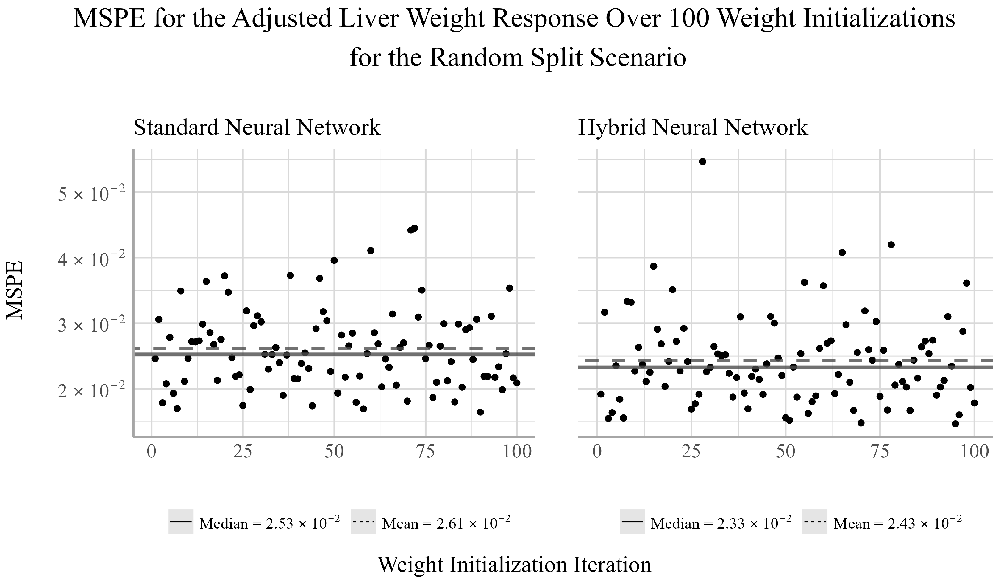
Mean square prediction error (MSPE) and MSE are two common metrics used to quantify model performance for continuous responses and were used to assess the predictive performance of the trained EN and NN models for this analysis. In the training of NNs, the node weight parameters (ws) require an initial value prior to training. These initial values are typically randomly selected and as such, the performance of the resulting NN model may vary based on how close these random values are to the optimal values. Finding the weights which result in the global minimum MSPE is not feasible, as there is an infinite number of possible initializations. A common approach to accounting for the variability of model performance induced by the random initialized weights is to ensemble the network. Ensembling a network involves fitting the same NN numerous times and combining the predictions from these NNs into a single prediction. 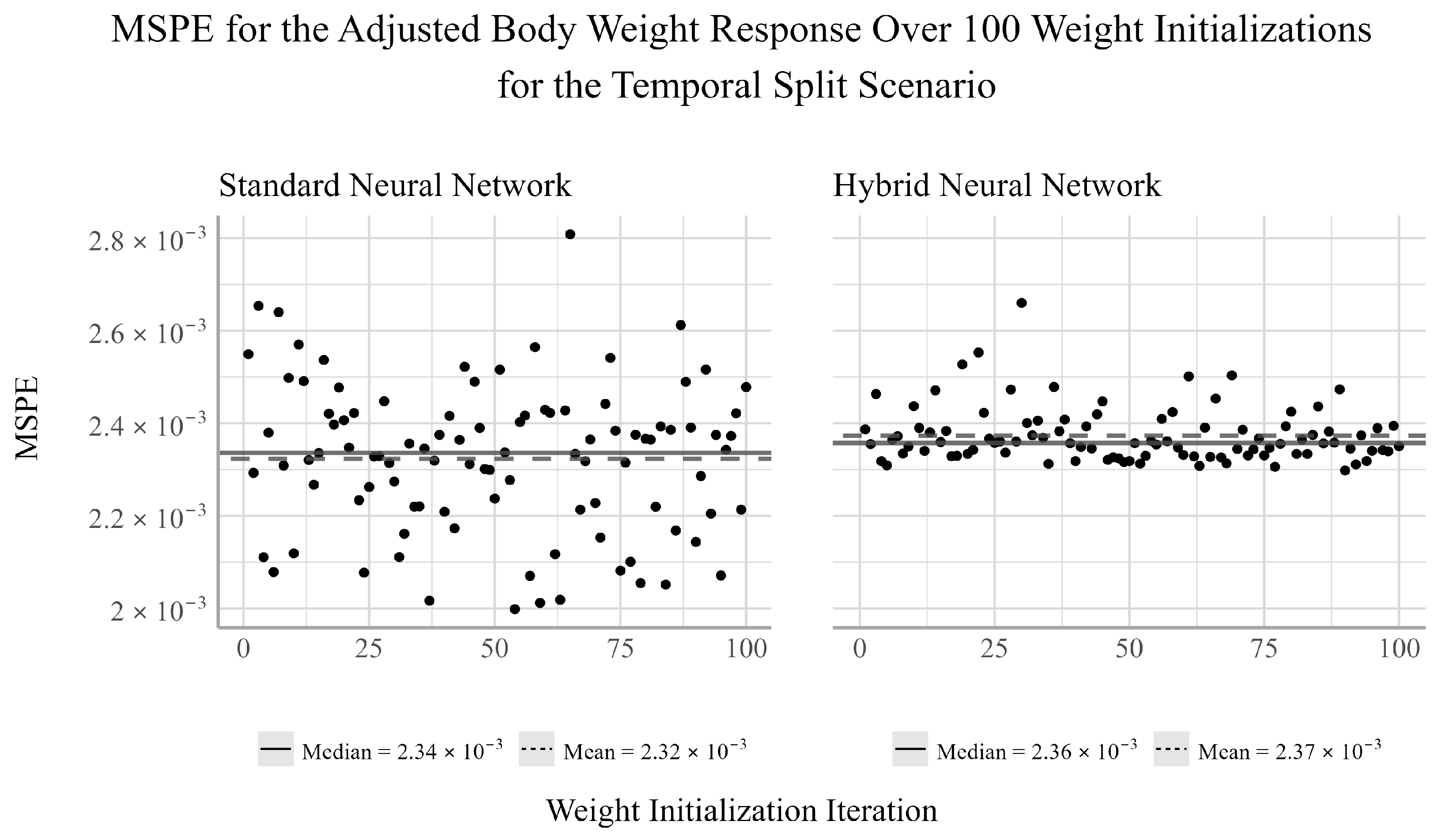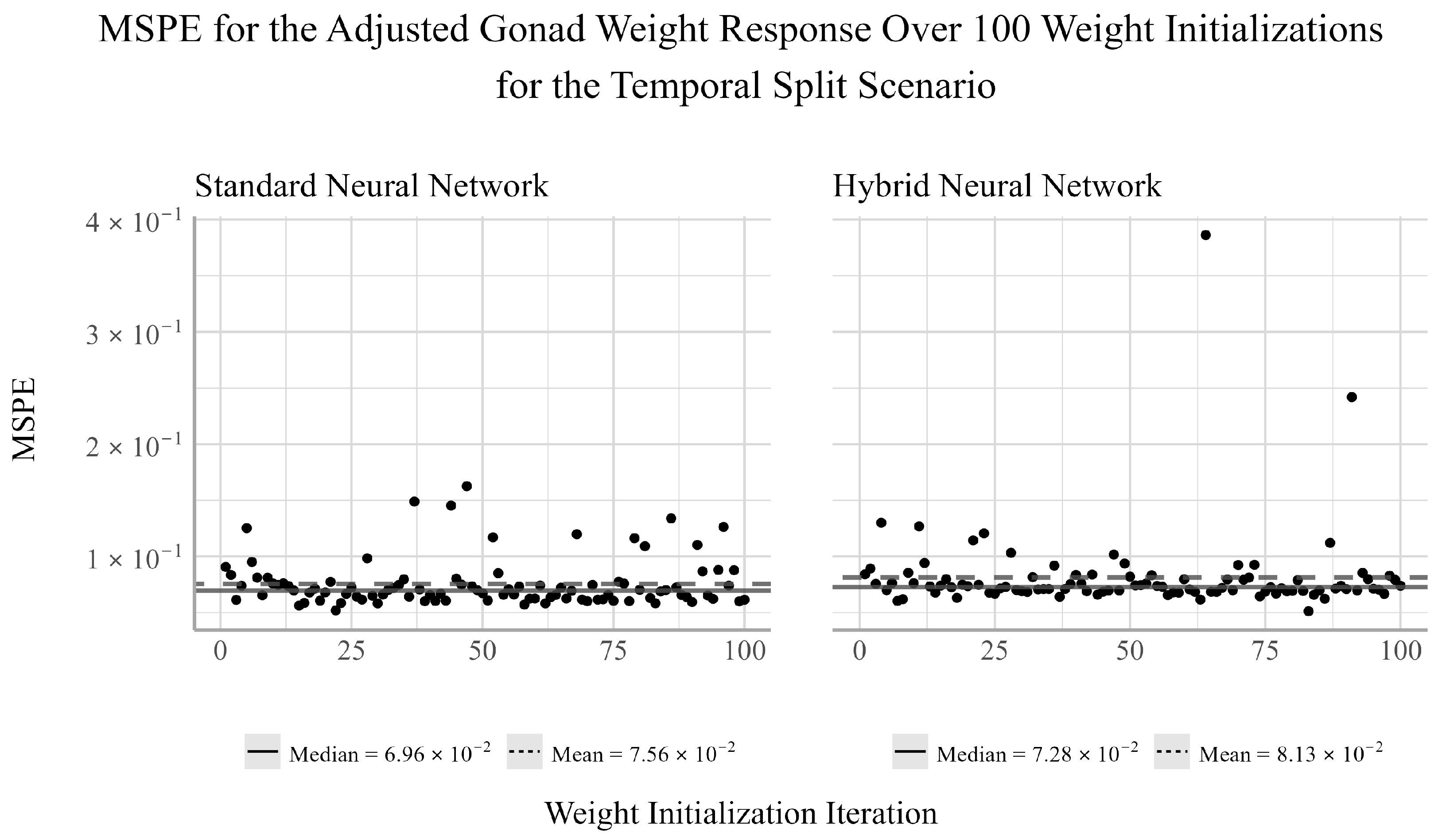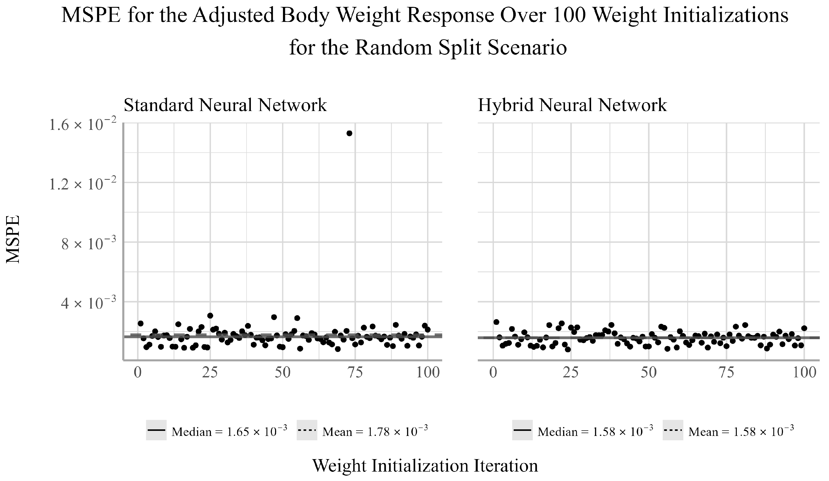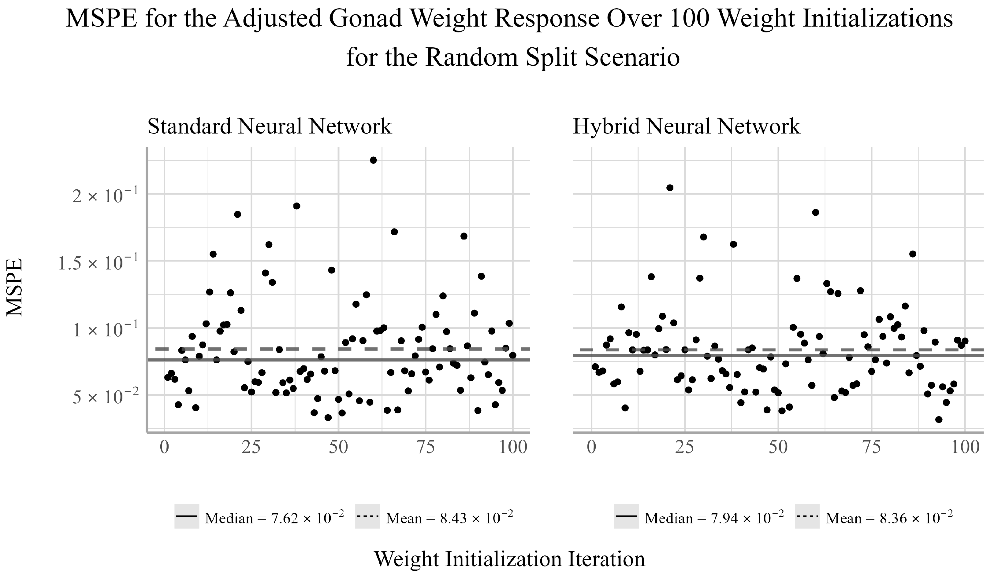This helps to reduce the variability of the prediction accuracy and can improve the model generalizability [38]. We chose to ensemble 100 randomly selected initializations for both NNs models considered in the analysis. For each initialization, there will be a pair of corresponding MSPE and MSE values for the trained model. Given that both MSPE and MSE have a lower bound of zero and the distributions of the MSPEs and MSEs were often not symmetric, the median of the MSPE and MSEs were used to assess the predictive performance of the ensemble NN models.

3. Results

3.1. Temporal Split Results

A summary of the performance of each model under the temporal split scenario is presented in

Table 1. Median values performance measures of each model by response for the temporal split scenario.

Response	Technique	MSPE	MSE
Adjusted Body Weight	EN	2.83 × 10−3	1.09 × 10−3
	NN	2.34 × 10−3	6.41 × 10−4
	Hybrid	2.36 × 10−3	7.00 × 10−4
Adjusted Gonad Weight	EN	1.02 × 10−1	5.05 × 10−2
	NN	6.96 × 10−2	3.30 × 10−2
	Hybrid	7.28 × 10−2	2.13 × 10−2
Adjusted Liver Weight	EN	2.29 × 10−2	2.28 × 10−2
	NN	4.83 × 10−2	1.41 × 10−2
	Hybrid	3.10 × 10−2	1.41 × 10−2

Bold values represent the best results for each metric and response.

. We find that for the adjusted body weight response, the standard NN had the smallest MSPE and MSE. The hybrid NN also achieved a comparably small MSPE. For the adjusted gonad weight response, the standard NN model was again found to have the smallest MSPE, followed by the hybrid NN and then the EN. Finally, for the adjusted liver weight response, the EN had the smallest MSPE, which was followed by the standard NN then hybrid NN. The three models performed similarly across the three response variables, with the exception of the adjusted gonad weight response, for which the EN model had an MSPE that was an order of magnitude larger than the standard NN and the hybrid NN. Of the two NN models, they had nearly identical MSPEs for the adjusted body weight response. The standard NN outperformed the hybrid NN for the adjusted gonad weight, but was outperformed by the hybrid NN for the adjusted liver weight response. As such, there does not appear to be any consistent advantage in terms of accuracy with regard to using one network over the other in this scenario.

To investigate the influence of the randomized initial weights of the NNs on model performance, we plotted the MSPE from each of the 100 weight initializations for both the standard and the hybrid NN and overlaid the mean and median values for each response variable. In Figure 1, we see the performance of the standard and hybrid NNs over the 100 random weight initializations for the adjusted body weight response. We find that the mean and median for each networks are similar, suggesting that the performances of the networks are distributed approximately uniformly. Comparing the range of the MSPE of the two networks, we find that the standard NN has a noticeably larger variance, suggesting that the hybrid NN is more stable in this scenario.

From Figure 2, we see that for both the standard and hybrid networks, the mean is larger than the median, suggesting a positive skew in the performance of the networks for this response. This skew is also evidenced by the apparent outliers in the model’s MSPE. The hybrid NN appears to be more susceptible to extreme deviations in performance, whereas the standard NN has more frequent, but less severe deviations in performance for this response.

Finally, from Figure 3, we see that for the standard NN, the mean is smaller than the median, suggesting a negative skew in the performance of this network for this response. This skew is also noticeable in terms of the inconsistent performance across the different weight initializations, which suggests that the random initialized weights can greatly influence the performance of the model. For the hybrid NN, we find that the mean is larger than the median, indicating a positive skew to the performance of this model. As is the case for the performance of the hybrid NN for the adjusted gonad weight response, we find that there are consistent outliers in model performance. The performance of the hybrid NN appears to be more susceptible to changes in the weight initialization. Despite this, the hybrid NN outperforms the standard NN by a considerable amount for the liver weight response, suggesting that variable selection prior to fitting a NN may reduce the model’s stability, but improve the average performance when ensembling under certain conditions.

3.2. Random Split Results

As is the case for the temporal split scenario, we fit each NN 100 times on the training set to assess the influence of the randomized weights on model performance on the test set. In this scenario, the training and testing sets were split randomly for each weight initialization. Each year–location combination was considered to be a unique environment and for each train–test split, 70% of environments were randomly selected to be used as the training set and the remaining 30% of environments were reserved as the test set. The random split scenario allowed us to assess model performance across a variety of spatial and temporal combinations, which provided better insight into the generalizability of these models. The EN model was also fit for each of the 100 train–test splits for comparison.

The median MSPE and MSE are presented for the three models across all response variables in

Table 2. Median values performance measures of each model by response for the random split scenario.

Response	Technique	MSPE	MSE
Adjusted Body Weight	EN	1.95 × 10−3	1.43 × 10−3
	NN	1.65 × 10−3	7.52 × 10−4
	Hybrid	1.58 × 10−3	7.79 × 10−4
Adjusted Gonad Weight	EN	7.13 × 10−2	5.24 × 10−2
	NN	7.62 × 10−2	2.90 × 10−2
	Hybrid	7.94 × 10−2	2.55 × 10−2
Adjusted Liver Weight	EN	2.67 × 10−2	2.21 × 10−2
	NN	2.53 × 10−2	1.35 × 10−2
	Hybrid	2.33 × 10−2	1.36 × 10−2

Bold values represent the best results for each metric and response.

. For the adjusted body-weight response, we see that the hybrid NN has the smallest median MSPE and the EN has the largest. For the adjusted gonad weight response, we find that the EN achieves the lowest median MSPE and the hybrid NN achieves the largest. Finally, for the adjusted liver weight, we see that again, the hybrid NN has the smallest median MSPE and the EN has the largest. Interestingly, the standard NN performed relatively conservatively, being neither worst nor best for any of the three response variables. These results suggest that variable selection prior to fitting the NN model can improve accuracy of the network across a more diverse set of testing scenarios relative to the temporal split scenario.

Comparing the performance of the two NN models across all 100 train–test split scenarios, from Figure 4, we see the performance of the standard and hybrid NNs have relatively little variation in performance, aside from a single outlier in the standard NN model’s performance. We see that the mean and median of the hybrid NN are the same, suggesting that the model’s performance is uniformly distributed. The presence of the outlier in the standard NN may suggest that variable selection prior to model fit can help guard against large variations in model performance as a result of the randomized weight initialization process under certain scenarios.

For the adjusted gonad weight response, from Figure 5 we can see that the mean of both networks is larger than the median, suggesting that the model performance has a positive skew. There does not appear to be any noticeable difference in the variability of the model performance between the two networks in this scenario.

Finally, from Figure 6, we find that for the adjusted liver weight response, the mean performance of both networks is again larger than the median performance, suggesting a positive skew. Additionally, the hybrid NN has larger outliers than the standard NN, but still achieves a smaller MSPE on average. This may suggest that the hybrid network is more prone to larger outliers, but is on average more accurate across a wider array of testing scenarios.

4. Discussion

The purpose of this analysis was to determine if nonlinear techniques such as NNs could produce more accurate predictions of several trout-perch health metrics relative to simpler, but more interpretable techniques such as the EN. Our results find that for the temporal split scenario, the EN outperforms the NNs in predicting the adjusted liver weight responses, but is outperformed by the NNs for the adjusted body and gonad weights. However, as the temporal split only considered a single year in the testing set, the results of this analysis may not be indicative of their generalized predictive ability.

From the random split analysis, we can gain a better idea of how well each of the models generalize to different training and testing scenarios. From this analysis, we found that the EN outperformed the NN models for the adjusted gonad weight response, but was outperformed by the NNs for the adjusted body and liver weight responses. The results from the temporal and random split scenarios may suggest that linear models can be sufficient for modeling the relationship between the development and health of the gonads and livers of trout-perch and the quality of the environment in which they reside. However, linear models appear to be less capable of accurately capturing the relationship between water quality variables and the overall body weight of the fish relative to nonlinear modeling techniques.

The adjusted body weight was best predicted by the NNs for both the temporal and random split scenarios, with the hybrid having the smallest MSPE for the random split scenario and the standard NN obtaining a slightly smaller MSPE than the hybrid NN for the temporal split scenario. It is well known that the effects of some water quality variables are dependent on their interaction with other variables in the environment [39,40]. Because of these interactions, we suspected this relationship was highly nonlinear and thus, implementing techniques such as NNs would result in improved prediction accuracy. Previous research has determined that while the EN did improve the model performance over the existing modeling techniques for the adjusted body weight of trout-perch, it did so to a much smaller extent than the performance increases seen for the adjusted gonad weight and adjusted liver weight responses [10]. This could suggest that the water quality variables influencing the overall body weight of trout-perch may interact with other variables, resulting in a complex, nonlinear system that linear models cannot accurately capture. This may explain the performance difference between the EN and NN models for the body weight response.

Between the two NN techniques considered, the hybrid method of using EN to select the explanatory variables to be used in the NN outperformed the NN fit using all available explanatory variables in two out of the four cases in which the NNs outperformed the EN. In one of two cases in which the standard NN outperformed the hybrid NN, the performance difference between the two models was very small. Furthermore, the variability of the hybrid NN’s performance relative to the standard NN’s was smaller in two of the six tests, equivalent in one, and larger in three. This indicates that variable selection may negatively impact the stability of the NN’s performance for individual weight initializations. However, when ensembling the network’s estimates, the median performance is on average more accurate than the standard NN. This result suggests that conducting feature selection prior to fitting the NNs may help to reduce overfitting and improve prediction accuracy when working with small datasets such as this.

Environmental effects monitoring programs are often multifaceted with respect to their objectives. The methods employed to achieve these objectives are similarly diverse. Methods such as NNs may be most appropriate for certain objectives when specific knowledge of systems drivers is not needed. However, outside of these scenarios, more suitable methods often exist. Techniques such as NNs have been applied to many complex problems with the goal of informing management decisions. However, many of these studies are either not interested in a mechanistic explanation of the system considered, or the system is already well defined. For instance, Bhullar et al. (2023) [41] investigated the use of deep-NNs for assessing how land suitability will change due to the effects of climate change. In this scenario, the system being analyzed, and the relationship between the environment and land suitability, is well understood, and so model accuracy is prioritized over interpretability [41]. In the context of problems in which high prediction accuracy is a priority but the underlying mechanism of the system is not well understood, hybridized analysis techniques such as those presented in this paper can bridge interpretable process-based models and less interpretable, but highly accurate machine learning models. While various causal inference techniques using machine learning are being developed for use in monitoring programs, the adoption of these techniques has been gradual [42]. We hope this paper serves to highlight the power and utility of these techniques, along with the motivation for implementing them into existing monitoring programs.

Incorporating NN models into a cohesive environmental monitoring framework could greatly benefit existing monitoring programs, as routine surveillance programs can generate vast quantities of data. Better predictions of fish health can work to improve the resiliency of early warning systems for environmental degradation by offering greater sensitivity to changes in water chemistry. While these models would not be used to determine a causal relationship, they can provide an initial estimate of which water quality variables may be driving changes in the health of a fish population. Based on this information, more detailed studies can be designed to determine if this relationship remains, if it is causal, to potentially identify sources of these variables, and also to potentially justify detailed and onerous investigation of solutions [43]. It is important to remember that these techniques serve as a single tool within the overall framework of environmental monitoring programs, and while they can improve early warning systems, they must be used in conjunction with other methods and approaches to ensure the health of the environment is sustained or improved.

In terms of the interpretability–performance trade-off of the methods considered, we see that each of the three models achieved the lowest MSPE in two out of six cases. However, in one case, when the standard NN outperformed the hybrid NN, the hybrid had very similar accuracy. As such, the hybrid NN would be preferable to the standard NN for this application, as there is no consistent advantage to one over the other in this study, but the hybrid NN does allow for some level of interpretation into which water quality variables may be influencing the response variables. Additionally, as the hybrid NN out performed the EN in four of the six test cases, we believe the increase in model accuracy outweighs the loss of interpretability for this application. As such, we find that the hybrid NN offers the best solution to the interpretability–performance trade-off issue when calculating normal ranges for environmental monitoring studies.

5. Conclusions

In this paper, we explore the application of NNs in predicting fish endpoints for obtaining more accurate normal ranges in monitoring programs in which no prior baseline has been established. While accurate normal ranges are essential to an effective monitoring program, it is also critical to understand the key explanatory variables that are driving changes in the response variables. We build an EN and two NN models to predict the adjusted body weight, adjusted gonad weight, and adjusted liver weight of trout-perch from the Athabasca River using water quality variables. We find that the two NN models can provide more accurate predictions of fish endpoints than the EN in both testing scenarios, and in cases in which the EN outperforms the NNs, the difference in accuracy is small. Additionally, the hybrid NN technique consistently provides more accurate, or comparably accurate, predictions of fish endpoints relative to the EN and standard NN techniques while being more interpretable than the standard NN. As such, the hybrid NN technique provides an optimal interpretability–performance trade-off of the models considered in this analysis.

This work also highlights the need for consistent and congruent data collection in environmental monitoring studies. As the years and locations of fish sampling did not line up perfectly with the years and sites of water sampling, information was likely lost during the amalgamation process. This additional information may have provided better insight into the driving factors influencing aquatic ecosystem health in the Athabasca OSR. A synergy between water quality data collection and sentinel species data collection may allow for more powerful statistical analysis to be conducted, which may help to more accurately model response variation and identify potential causes.

This paper serves as an introduction to applications of machine learning in environmental monitoring studies. Future work should consider other machine learning models, such as Random Forests (RFs), or other classification and regression tree (CART)-based models. Tree-based methods may present a better balance of predictive performance and interpretability. While feature importance can be derived from NNs, many tree-based methods are able to perform this automatically. In particular, RFs may see success in this application, as all observations in a particular region are given the same prediction (the mean), and all fish in the same region share the same water quality variables. Therefore, the best any model can do is predict the mean of a particular group as accurately as possible. Furthermore, tree-based methods such as RFs are nonlinear and can also capture complex interactions among variables, which may make them appropriate for this application.