
Scrutinizing the Statistical Distribution of a Composite Index of Soil Degradation as a Measure of Early Desertification Risk in Advanced Economies

 , ,
, , 

Abstract
1. Introduction
2. Methodology
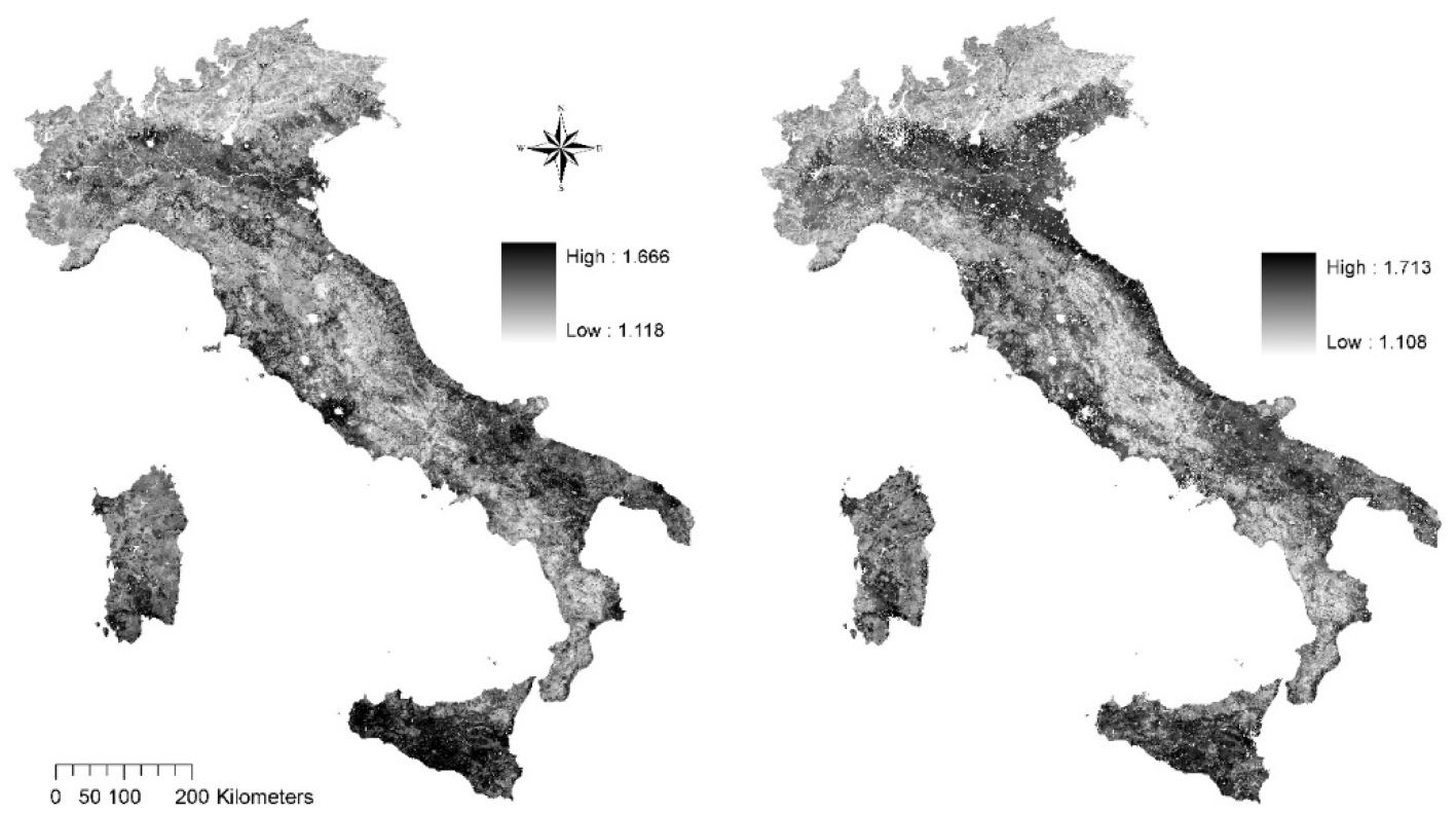
2.1. Study Area
2.2. Data and Variables
2.3. Indicators and Future Scenarios
2.4. Data Analysis
Multidimensional Analysis
3. Results
3.1. A Descriptive Analysis of a Composite Index of Soil Degradation
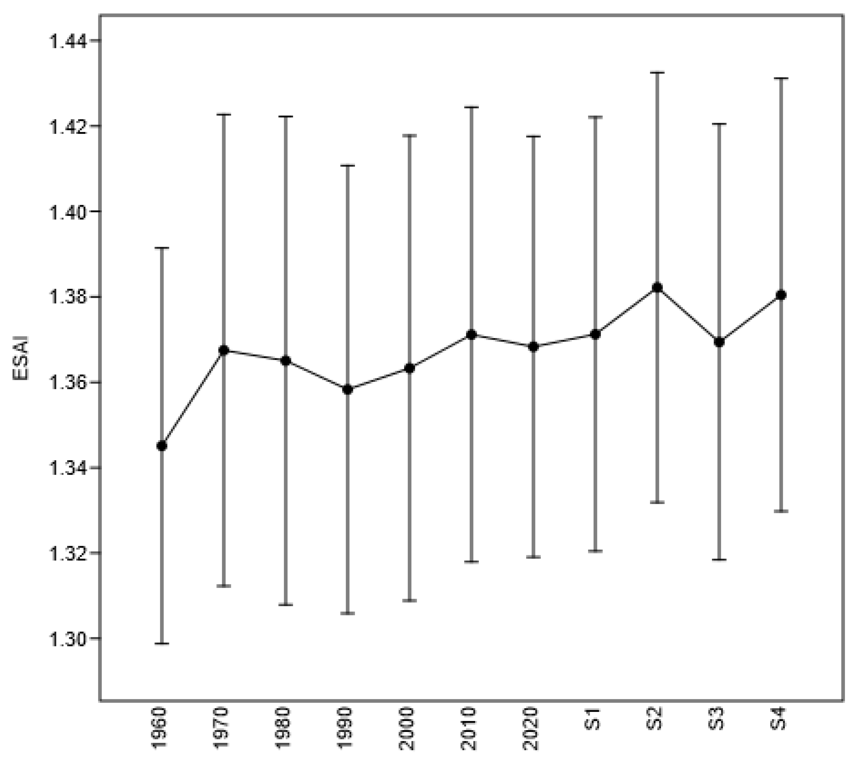
3.2. Distributional Metrics Delineating Trends over Time in a Composite Index of Soil Degradation
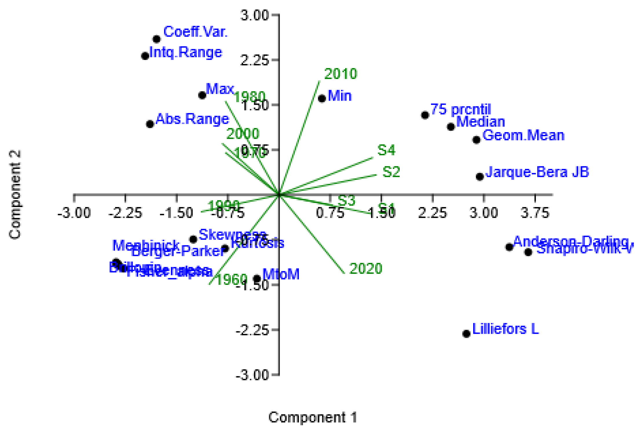
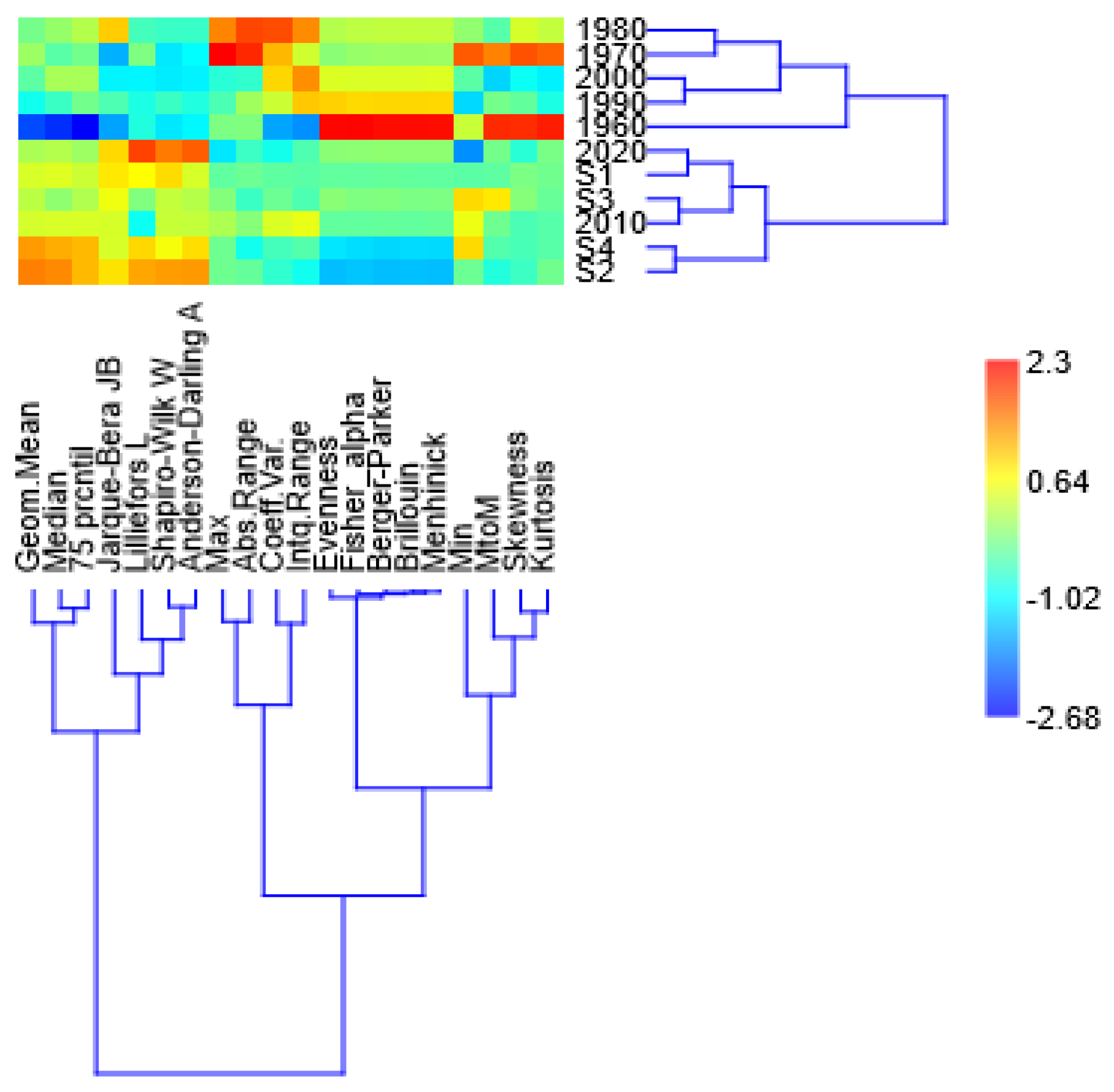
3.3. A Multivariate Analysis of Distributional Metrics in a Composite Index of Soil Degradation
4. Discussion
5. Conclusions
Author Contributions
Funding
Data Availability Statement
Conflicts of Interest
References
- Abahussain, A.A.; Abdu, A.S.; Al-Zubari, W.K.; El-Deen, N.A.; Abdul-Raheem, M. Desertification in the Arab Region: Analysis of current status and trends. J. Arid Environ. 2002, 51, 521–545. [Google Scholar] [CrossRef]
- Amiraslani, F.; Dragovich, D. Combating desertification in Iran over the last 50 years: An overview of changing approaches. J. Environ. Manag. 2011, 92, 1–13. [Google Scholar] [CrossRef] [PubMed]
- Assennato, F.; Smiraglia, D.; Cavalli, A.; Congedo, L.; Giuliani, C.; Riitano, N.; Strollo, A.; Munafò, M. The Impact of Urbanization on Land: A Biophysical-Based Assessment of Ecosystem Services Loss Supported by Remote Sensed Indicators. Land 2022, 11, 236. [Google Scholar] [CrossRef]
- Martinho, V.J.P.D. European Union farming systems: Insights for a more sustainable land use. Land Degrad. Dev. 2022, 33, 527–544. [Google Scholar] [CrossRef]
- Becerril-Piña, R.; Mastachi-Loza, C.A.; González-Sosa, E.; Díaz-Delgado, C.; Bâ, K.M. Assessing desertification risk in the semi-arid highlands of central Mexico. J. Arid Environ. 2015, 120, 4–13. [Google Scholar] [CrossRef]
- Bestelmeyer, B.T.; Okin, G.S.; Duniway, M.C.; Archer, S.R.; Sayre, N.F.; Williamson, J.C.; Herrick, J.E. Desertification, land use, and the transformation of global drylands. Front. Ecol. Environ. 2015, 13, 28–36. [Google Scholar] [CrossRef]
- Briassoulis, H. Governing desertification in Mediterranean Europe: The challenge of environmental policy integration in multi-level governance contexts. Land Degrad. Dev. 2011, 22, 313–325. [Google Scholar] [CrossRef]
- Bojö, J. The costs of land degradation in Sub-Saharan Africa. Ecol. Econ. 1996, 16, 161–173. [Google Scholar] [CrossRef]
- Davison, C.W.; Rahbek, C.; Morueta-Holme, N. Land-use change and biodiversity: Challenges for assembling evidence on the greatest threat to nature. Glob. Change Biol. 2021, 27, 5414–5429. [Google Scholar] [CrossRef]
- Barbero-Sierra, C.; Marques, M.J.; Ruíz-Pérez, M. The case of urban sprawl in Spain as an active and irreversible driving force for desertification. J. Arid Environ. 2013, 90, 95–102. [Google Scholar] [CrossRef]
- Danfeng, S.; Dawson, R.; Baoguo, L. Agricultural causes of desertification risk in Minqin, China. J. Environ. Manag. 2006, 79, 348–356. [Google Scholar] [CrossRef] [PubMed]
- Van Vliet, J.; de Groot, H.L.; Rietveld, P.; Verburg, P.H. Manifestations and underlying drivers of agricultural land use change in Europe. Landsc. Urban Plan. 2015, 133, 24–36. [Google Scholar] [CrossRef]
- Cecchini, M.; Zambon, I.; Pontrandolfi, A.; Turco, R.; Colantoni, A.; Mavrakis, A.; Salvati, L. Urban sprawl and the ‘olive’ landscape: Sustainable land management for ‘crisis’ cities. GeoJournal 2019, 84, 237–255. [Google Scholar] [CrossRef]
- De Fioravante, P.; Strollo, A.; Cavalli, A.; Cimini, A.; Smiraglia, D.; Assennato, F.; Munafò, M. Ecosystem Mapping and Accounting in Italy Based on Copernicus and National Data through Integration of EAGLE and SEEA-EA Frameworks. Land 2023, 12, 286. [Google Scholar] [CrossRef]
- Ciommi, M.; Chelli, F.; Carlucci, M.; Salvati, L. Urban Growth and Demographic Dynamics in Southern Europe: Toward a New Statistical Approach to Regional Science. Sustainability 2018, 10, 2765. [Google Scholar] [CrossRef]
- Colantoni, A.; Mavrakis, A.; Sorgi, T.; Salvati, L. Towards a ‘polycentric’ landscape? Reconnecting fragments into an integrated network of coastal forests in Rome. Rend. Lincei 2015, 26, 615–624. [Google Scholar] [CrossRef]
- Gomes, E.; Inácio, M.; Bogdzevič, K.; Kalinauskas, M.; Karnauskaitė, D.; Pereira, P. Future land-use changes and its impacts on terrestrial ecosystem services: A review. Sci. Total Environ. 2021, 781, 146716. [Google Scholar] [CrossRef]
- Basso, F.; Bove, E.; Dumontet, S.; Ferrara, A.; Pisante, M.; Quaranta, G.; Taberner, M. Evaluating environmental sensitivity at the basin scale through the use of geographic information systems and remotely sensed data: An example covering the Agri basin (Southern Italy). Catena 2000, 40, 19–35. [Google Scholar] [CrossRef]
- Briassoulis, H. The institutional complexity of environmental policy and planning problems: The example of Mediterranean desertification. J. Environ. Plan. Manag. 2006, 47, 115–135. [Google Scholar] [CrossRef]
- De Groot, R. Function-analysis and valuation as a tool to assess land use conflicts in planning for sustainable, multi-functional landscapes. Landsc. Urban Plan. 2006, 75, 175–186. [Google Scholar] [CrossRef]
- Fernández, R.J. Do humans create deserts? Trends Ecol. Evol. 2002, 17, 6–7. [Google Scholar] [CrossRef]
- Kuemmerle, T.; Levers, C.; Erb, K.; Estel, S.; Jepsen, M.R.; Müller, D.; Reenberg, A. Hotspots of land use change in Europe. Environ. Res. Lett. 2016, 11, 064020.23. [Google Scholar] [CrossRef]
- Gisladottir, G.; Stocking, M. Land degradation control and its global environmental benefits. Land Degrad. Dev. 2005, 16, 99–112. [Google Scholar] [CrossRef]
- Delfanti, L.; Colantoni, A.; Recanatesi, F.; Bencardino, M.; Sateriano, A.; Zambon, I.; Salvati, L. Solar plants, environmental degradation and local socioeconomic contexts: A case study in a Mediterranean country. Environ. Impact Assess. Rev. 2016, 61, 88–93. [Google Scholar] [CrossRef]
- Juntti, M.; Wilson, G.A. Conceptualizing desertification in Southern Europe: Stakeholder interpretations and multiple policy agendas. Eur. Environ. 2005, 15, 228–249. [Google Scholar] [CrossRef]
- Hein, L. Assessing the costs of land degradation: A case study for the Puentes catchment, southeast Spain. Land Degrad. Dev. 2007, 18, 631–642. [Google Scholar] [CrossRef]
- Iosifides, T.; Politidis, T. Socio-economic dynamics, local development and desertification in western Lesvos, Greece. Local Environ. 2006, 10, 487–499. [Google Scholar] [CrossRef]
- Hammad, A.A.; Tumeizi, A. Land degradation: Socioeconomic and environmental causes and consequences in the eastern Mediterranean. Land Degrad. Dev. 2012, 23, 216–226. [Google Scholar] [CrossRef]
- Ibáñez, J.; Valderrama, J.M.; Puigdefábregas, J. Assessing desertification risk using system stability condition analysis. Ecol. Model. 2008, 213, 180–190. [Google Scholar] [CrossRef]
- Kairis, O.; Karavitis, C.; Kounalaki, A.; Salvati, L.; Kosmas, C. The effect of land management practices on soil erosion and land desertification in an olive grove. Soil Use Manag. 2013, 29, 597–606. [Google Scholar] [CrossRef]
- Ferrara, A.; Kosmas, C.; Salvati, L.; Padula, A.; Mancino, G.; Nolè, A. Updating the MEDALUS-ESA Framework for Worldwide Land Degradation and Desertification Assessment. Land Degrad. Dev. 2020, 31, 1593–1607. [Google Scholar] [CrossRef]
- Kok, K.; Patel, M.; Rothman, D.; Quaranta, G. Multi-scale narratives from an IA perspective: Part II. Participatory local scenario development. Futures 2006, 38, 285–311. [Google Scholar] [CrossRef]
- Kosmas, C.; Tsara, M.; Karavitis, C.A. Identification of indicators for desertification effects of using treated municipal waste water for irrigation of olive trees in Greece. Ann. Arid Zones 2003, 42, 393–416. [Google Scholar]
- Rabbinge, R.; Van Diepen, C.A. Changes in agriculture and land use in Europe. Eur. J. Agron. 2000, 13, 85–99. [Google Scholar] [CrossRef]
- Lambin, E.F.; Meyfroidt, P. Land Use Transitions: Socio-Ecological Feedback versus Socio-Economic Change. Land Use Policy 2010, 27, 108–118. [Google Scholar] [CrossRef]
- Galeotti, M. Economic growth and the quality of the environment: Taking stock. Environ. Dev. Sustain. 2007, 9, 427–454. [Google Scholar] [CrossRef]
- Dierwechter, Y. Metropolitan geographies of US climate action: Cities, suburbs, and the local divide in global responsibilities. J. Environ. Policy Plan. 2010, 12, 59–82. [Google Scholar] [CrossRef]
- Bouma, J.; Varallyay, G.; Batjes, N.H. Principal land use changes anticipated in Europe. Agric. Ecosyst. Environ. 1998, 67, 103–119. [Google Scholar] [CrossRef]
- Reginster, I.; Rounsevell, M. Scenarios of future urban land use in Europe. Environ. Plan. B Plan. Des. 2006, 33, 619–636. [Google Scholar] [CrossRef]
- Imeson, A. Desertification, Land Degradation and Sustainability; Wiley: London, UK, 2012. [Google Scholar]
- Grainger, A. The role of science in implementing international environmental agreements: The case of desertification. Land Degrad. Dev. 2009, 20, 410–430. [Google Scholar] [CrossRef]
- Herrmann, S.M.; Hutchinson, C.F. The changing contexts of the desertification debate. J. Arid Environ. 2005, 63, 538–555. [Google Scholar] [CrossRef]
- Hubacek, K.; Van Den Bergh, J.C.J.M. Changing concepts of ‘land’ in economic theory: From single to multi-disciplinary approaches. Ecol. Econ. 2006, 56, 5–27. [Google Scholar] [CrossRef]
- Jiang, Y.; Tang, Y.T.; Long, H.; Deng, W. Land consolidation: A comparative research between Europe and China. Land Use Policy 2022, 112, 105790. [Google Scholar] [CrossRef]
- Castillo, C.P.; Jacobs-Crisioni, C.; Diogo, V.; Lavalle, C. Modelling agricultural land abandonment in a fine spatial resolution multi-level land-use model: An application for the EU. Environ. Model. Softw. 2021, 136, 104946. [Google Scholar] [CrossRef] [PubMed]
- Seto, K.C.; Sánchez-Rodríguez, R.; Fragkias, M. The new geography of contemporary urbanization and the environment. Annu. Rev. Environ. Resour. 2010, 35, 167–194. [Google Scholar] [CrossRef]
- Patel, M.; Kok, K.; Rothman, D.S. Participatory scenario construction in land use analysis: An insight into the experiences created by stakeholder involvement in the Northern Mediterranean. Land Use Policy 2007, 24, 546–561. [Google Scholar] [CrossRef]
- Hoffmann, P.; Reinhart, V.; Rechid, D.; de Noblet-Ducoudré, N.; Davin, E.L.; Asmus, C.; Luyssaert, S. High-resolution land use and land cover dataset for regional climate modelling: Historical and future changes in Europe. Earth Syst. Sci. Data Discuss. 2022, 15, 3819–3852. [Google Scholar] [CrossRef]
- Salvati, L.; Zitti, M. Land degradation in the Mediterranean basin: Linking bio-physical and economic factors into an ecological perspective. Biota 2005, 5, 67–77. [Google Scholar]
- Scarascia, M.E.V.; Di Battista, F.; Salvati, L. Water resources in Italy: Availability and agricultural uses. Irrig. Drain. 2006, 55, 115–127. [Google Scholar] [CrossRef]
- Marathianou, M.; Kosmas, C.; Detsis, V. Land-use evolution and degradation in Lesvos (Greece): A historical approach. Land Degrad. Dev. 2000, 11, 63–73. [Google Scholar] [CrossRef]
- Makhzoumi, J.M. The changing role of rural landscapes: Olive and carob multi-use tree plantations in the semiarid Mediterranean. Landsc. Urban Plan. 1997, 37, 115–122. [Google Scholar] [CrossRef]
- Otto, R.; Krüsi, B.O.; Kienast, F. Degradation of an arid coastal landscape in relation to land use changes in Southern Tenerife (Canary Islands). J. Arid Environ. 2007, 70, 527–539. [Google Scholar] [CrossRef]
- Loumou, A.; Giourga, C.; Dimitrakopoulos, P.; Koukoulas, S. Tourism contribution to agro-ecosystems conservation: The case of Lesbos Island, Greece. Environ. Manag. 2000, 26, 363–370. [Google Scholar] [CrossRef]
- Lemon, M.; Seaton, R.; Park, J. Social enquiry and the measurement of natural phenomena: The degradation of irrigation water in the Argolid Plain, Greece. Int. J. Sustain. Dev. World Ecol. 2009, 1, 206–220. [Google Scholar] [CrossRef]
- Portnov, B.A.; Safriel, U.N. Combating desertification in the Negev: Dryland agriculture vs. dryland urbanization. J. Arid Environ. 2004, 56, 659–680. [Google Scholar] [CrossRef]
- Fayet, C.M.; Reilly, K.H.; Van Ham, C.; Verburg, P.H. What is the future of abandoned agricultural lands? A systematic review of alternative trajectories in Europe. Land Use Policy 2022, 112, 105833. [Google Scholar] [CrossRef]
- Tanrivermis, H. Agricultural land use change and sustainable use of land resources in the Mediterranean region of Turkey. J. Arid Environ. 2003, 54, 553–564. [Google Scholar] [CrossRef]
- Le Houérou, H.N. Land degradation in Mediterranean Europe: Can agroforestry be a part of the solution? A prospective review. Agrofor. Syst. 1993, 21, 43–61. [Google Scholar] [CrossRef]
- Verstraete, M.M.; Brink, A.B.; Scholes, R.J.; Beniston, M.; Stafford Smith, M. Climate change and desertification: Where do we stand, where should we go? Glob. Planet. Change 2008, 64, 105–110. [Google Scholar] [CrossRef]
- Rubio, J.L.; Bochet, E. Desertification indicators as diagnosis criteria for desertification risk assessment in Europe. J. Arid Environ. 1998, 39, 113–120. [Google Scholar] [CrossRef]
- Perrin, C.; Nougarèdes, B.; Sini, L.; Branduini, P.; Salvati, L. Governance changes in peri-urban farmland protection following decentralisation: A comparison between Montpellier (France) and Rome (Italy). Land Use Policy 2018, 70, 535–546. [Google Scholar] [CrossRef]
- Recanatesi, F.; Clemente, M.; Grigoriadis, E.; Ranalli, F.; Zitti, M.; Salvati, L. A fifty-year sustainability assessment of Italian agro-forest districts. Sustainability 2016, 8, 32. [Google Scholar] [CrossRef]
- Modica, G.; Vizzari, M.; Pollino, M.; Fichera, C.R.; Zoccali, P.; Di Fazio, S. Spatio-temporal analysis of the urban–rural gradient structure: An application in a Mediterranean mountainous landscape. Earth Syst. Dyn. 2012, 3, 263–279. [Google Scholar] [CrossRef]
- Oñate, J.J.; Peco, B. Policy impact on desertification: Stakeholders’ perceptions in southeast Spain. Land Use Policy 2005, 22, 103–114. [Google Scholar] [CrossRef]
- Salvati, L.; Zambon, I.; Chelli, F.M.; Serra, P. Do spatial patterns of urbanization and land consumption reflect different socioeconomic contexts in Europe? Sci. Total Environ. 2018, 625, 722–730. [Google Scholar] [CrossRef]
- Safriel, U.; Adeel, Z. Development paths of drylands: Thresholds and sustainability. Sustain. Sci. 2008, 3, 117–123. [Google Scholar] [CrossRef]
- Wang, X.; Chen, F.; Dong, Z. The relative role of climatic and human factors in desertification in semiarid China. Glob. Environ. Change 2006, 16, 48–57. [Google Scholar] [CrossRef]
- Prishchepov, A.V.; Müller, D.; Dubinin, M.; Baumann, M.; Radeloff, V.C. Determinants of agricultural land abandonment in post-Soviet European Russia. Land Use Policy 2013, 30, 873–884. [Google Scholar] [CrossRef]
- Egidi, G.; Salvati, L.; Vinci, S. The long way to tipperary: City size and worldwide urban population trends, 1950–2030. Sustain. Cities Soc. 2020, 60, 102148. [Google Scholar] [CrossRef]
- Elmqvist, T.; Fragkias, M.; Goodness, J.; Güneralp, B.; Marcotullio, P.J.; McDonald, R.I.; Parnell, S.; Schewenius, M.; Sendstad, M.; Seto, K.C.; et al. Urbanization, Biodiversity and Ecosystem Services: Challenges and Opportunities; Springer: Utrecht, The Netherlands, 2013. [Google Scholar]
- Harte, J. Human population as a dynamic factor in environmental degradation. Popul. Environ. 2007, 28, 223–236. [Google Scholar] [CrossRef]
- Johnson, D.L.; Lewis, L.A. Land Degradation: Creation and Destruction, 2nd ed.; Rowman & Littlefield: Lahnam, MD, USA, 2007. [Google Scholar]
- Khresat, S.A.; Rawajfih, Z.; Mohammad, M. Land degradation in north-western Jordan: Causes and processes. J. Arid Environ. 1998, 39, 623–629. [Google Scholar] [CrossRef]
- Latorre, J.G.; García-Latorre, J.; Sanchez-Picón, A. Dealing with aridity: Socio-economic structures and environmental changes in an arid Mediterranean region. Land Use Policy 2001, 18, 53–64. [Google Scholar] [CrossRef]
- Yang, X.; Zhang, K.; Jia, B.; Ci, L. Desertification assessment in China: An overview. J. Arid Environ. 2005, 63, 517–531. [Google Scholar] [CrossRef]
- Zambon, I.; Benedetti, A.; Ferrara, C.; Salvati, L. Soil matters? A multivariate analysis of socioeconomic constraints to urban expansion in Mediterranean Europe. Ecol. Econ. 2018, 146, 173–183. [Google Scholar] [CrossRef]
- Zasada, I.; Loibl, W.; Köstl, M.; Piorr, A. Agriculture under human influence: A spatial analysis of farming systems and land use in European rural-urban-regions. Eur. Countrys. 2013, 5, 71–88. [Google Scholar] [CrossRef]
- Zuindeau, B. Territorial Equity and Sustainable Development. Environ. Values 2007, 16, 253–268. [Google Scholar] [CrossRef]
- Zucca, C.; Della Peruta, R.; Salvia, R.; Sommer, S.; Cherlet, M. Towards a World Desertification Atlas. Relating and selecting indicators and data sets to represent complex issues. Ecol. Indic. 2012, 15, 157–170. [Google Scholar] [CrossRef]


| Scenario | Increasing Climate Aridity | Demographic Dynamics | ||
|---|---|---|---|---|
| +5% | +10% | Stable | Increasing | |
| S1 | ● | ● | ||
| S2 | ● | ● | ||
| S3 | ● | ● | ||
| S4 | ● | ● | ||
| Statistic | 1960 | 1970 | 1980 | 1990 | 2000 | 2010 | 2020 | S1 | S2 | S3 | S4 |
|---|---|---|---|---|---|---|---|---|---|---|---|
| Min | 1.261 | 1.273 | 1.258 | 1.248 | 1.255 | 1.263 | 1.244 | 1.255 | 1.256 | 1.266 | 1.266 |
| Max | 1.487 | 1.542 | 1.523 | 1.480 | 1.475 | 1.494 | 1.466 | 1.483 | 1.485 | 1.488 | 1.485 |
| Mean | 1.345 | 1.367 | 1.365 | 1.358 | 1.363 | 1.371 | 1.368 | 1.371 | 1.382 | 1.369 | 1.380 |
| Median | 1.337 | 1.361 | 1.366 | 1.359 | 1.368 | 1.372 | 1.369 | 1.372 | 1.385 | 1.366 | 1.382 |
| MtoM | 1.006 | 1.004 | 0.999 | 0.999 | 0.996 | 0.999 | 0.999 | 0.999 | 0.998 | 1.002 | 0.998 |
| Geom. Mean | 1.344 | 1.366 | 1.364 | 1.357 | 1.362 | 1.370 | 1.367 | 1.370 | 1.381 | 1.368 | 1.379 |
| Coeff. Var. | 0.034 | 0.040 | 0.042 | 0.039 | 0.039 | 0.038 | 0.036 | 0.037 | 0.036 | 0.037 | 0.036 |
| Abs. Range | 0.168 | 0.197 | 0.194 | 0.171 | 0.161 | 0.168 | 0.162 | 0.166 | 0.165 | 0.162 | 0.158 |
| 25 prcntil | 1.309 | 1.321 | 1.319 | 1.317 | 1.317 | 1.327 | 1.330 | 1.333 | 1.345 | 1.332 | 1.342 |
| 75 prcntil | 1.375 | 1.403 | 1.408 | 1.403 | 1.407 | 1.411 | 1.406 | 1.410 | 1.419 | 1.408 | 1.419 |
| Intq. Range | 0.049 | 0.060 | 0.065 | 0.063 | 0.065 | 0.060 | 0.055 | 0.056 | 0.053 | 0.055 | 0.055 |
| Skewness | 0.728 | 0.657 | 0.242 | 0.0188 | −0.149 | −0.026 | −0.090 | 0.067 | −0.054 | 0.088 | −0.030 |
| Kurtosis | 0.412 | 0.213 | −0.396 | −0.866 | −0.984 | −0.701 | −0.602 | −0.628 | −0.627 | −0.655 | −0.699 |
| Inference | 1960 | 1970 | 1980 | 1990 | 2000 | 2010 | 2020 | S1 | S2 | S3 | S4 |
|---|---|---|---|---|---|---|---|---|---|---|---|
| Shapiro–Wilk W | 0.9623 | 0.9647 | 0.9801 | 0.9802 | 0.9684 | 0.9852 | 0.9887 | 0.9871 | 0.9882 | 0.9851 | 0.9862 |
| p (normal) | 0.0034 | 0.0051 | 0.0987 | 0.1005 | 0.0103 | 0.2669 | 0.4906 | 0.3742 | 0.4487 | 0.2631 | 0.3215 |
| Anderson–Darling A | 0.9838 | 0.8787 | 0.6150 | 0.6830 | 1.1520 | 0.4221 | 0.2770 | 0.4061 | 0.3069 | 0.4339 | 0.3547 |
| p (normal) | 0.0130 | 0.0237 | 0.1070 | 0.0725 | 0.0050 | 0.3164 | 0.6479 | 0.3454 | 0.5582 | 0.2966 | 0.4554 |
| p (Monte Carlo) | 0.0119 | 0.0252 | 0.1077 | 0.0744 | 0.0038 | 0.3220 | 0.6777 | 0.3485 | 0.5767 | 0.2895 | 0.4567 |
| Lilliefors L | 0.0785 | 0.0671 | 0.0730 | 0.0794 | 0.0913 | 0.0829 | 0.0473 | 0.0582 | 0.0531 | 0.0669 | 0.0559 |
| p (normal) | 0.0921 | 0.2515 | 0.1536 | 0.0851 | 0.0242 | 0.0597 | 0.7870 | 0.4691 | 0.6183 | 0.2567 | 0.5353 |
| p (Monte Carlo) | 0.0935 | 0.2599 | 0.1585 | 0.0861 | 0.0254 | 0.0642 | 0.7857 | 0.4899 | 0.6167 | 0.2597 | 0.5386 |
| Jarque–Bera JB | 9.9810 | 7.7950 | 1.9040 | 3.5670 | 4.9290 | 2.4170 | 1.9600 | 2.0440 | 2.0120 | 2.2580 | 2.4080 |
| p (normal) | 0.0068 | 0.0203 | 0.3859 | 0.1681 | 0.0851 | 0.2986 | 0.3752 | 0.3598 | 0.3657 | 0.3234 | 0.3000 |
| p (Monte Carlo) | 0.0153 | 0.0283 | 0.3118 | 0.1047 | 0.0652 | 0.2125 | 0.2931 | 0.2725 | 0.2840 | 0.2418 | 0.2143 |
| Metric | 1960 | 1970 | 1980 | 1990 | 2000 | 2010 | 2020 | S1 | S2 | S3 | S4 |
|---|---|---|---|---|---|---|---|---|---|---|---|
| Evenness | 1.4440 | 1.4350 | 1.4360 | 1.4390 | 1.4370 | 1.4340 | 1.4350 | 1.4340 | 1.4300 | 1.4350 | 1.4310 |
| Brillouin | 2.6380 | 2.5840 | 2.5900 | 2.6060 | 2.5940 | 2.5750 | 2.5820 | 2.5750 | 2.5500 | 2.5790 | 2.5540 |
| Menhinick | 9.0430 | 8.9690 | 8.9770 | 8.9990 | 8.9830 | 8.9570 | 8.9660 | 8.9560 | 8.9210 | 8.9620 | 8.9270 |
| Fisher_alpha | 194.20 | 184.40 | 185.40 | 188.30 | 186.20 | 182.90 | 184.10 | 182.90 | 178.60 | 183.70 | 179.30 |
| Berger-Parker | 0.0068 | 0.0066 | 0.0067 | 0.0067 | 0.0067 | 0.0066 | 0.0066 | 0.0066 | 0.0066 | 0.0066 | 0.0066 |
Disclaimer/Publisher’s Note: The statements, opinions and data contained in all publications are solely those of the individual author(s) and contributor(s) and not of MDPI and/or the editor(s). MDPI and/or the editor(s) disclaim responsibility for any injury to people or property resulting from any ideas, methods, instructions or products referred to in the content. |
© 2024 by the authors. Licensee MDPI, Basel, Switzerland. This article is an open access article distributed under the terms and conditions of the Creative Commons Attribution (CC BY) license (https://creativecommons.org/licenses/by/4.0/).
Share and Cite
Imbrenda, V.; Maialetti, M.; Sateriano, A.; Scarpitta, D.; Quaranta, G.; Chelli, F.; Salvati, L. Scrutinizing the Statistical Distribution of a Composite Index of Soil Degradation as a Measure of Early Desertification Risk in Advanced Economies. Environments 2024, 11, 246. https://doi.org/10.3390/environments11110246
Imbrenda V, Maialetti M, Sateriano A, Scarpitta D, Quaranta G, Chelli F, Salvati L. Scrutinizing the Statistical Distribution of a Composite Index of Soil Degradation as a Measure of Early Desertification Risk in Advanced Economies. Environments. 2024; 11(11):246. https://doi.org/10.3390/environments11110246
Chicago/Turabian StyleImbrenda, Vito, Marco Maialetti, Adele Sateriano, Donato Scarpitta, Giovanni Quaranta, Francesco Chelli, and Luca Salvati. 2024. "Scrutinizing the Statistical Distribution of a Composite Index of Soil Degradation as a Measure of Early Desertification Risk in Advanced Economies" Environments 11, no. 11: 246. https://doi.org/10.3390/environments11110246
APA StyleImbrenda, V., Maialetti, M., Sateriano, A., Scarpitta, D., Quaranta, G., Chelli, F., & Salvati, L. (2024). Scrutinizing the Statistical Distribution of a Composite Index of Soil Degradation as a Measure of Early Desertification Risk in Advanced Economies. Environments, 11(11), 246. https://doi.org/10.3390/environments11110246