Abstract
In urban areas, there has been a recent rise in ground-level ozone. Given its toxicity to both humans and the environment, the investigation of ozone pollution demands attention and should not be overlooked. Therefore, we conducted a study on ozone concentration in three distinct locations within the city of Magurele, Romania. This investigation considered variations in both structure and location during the spring and summer seasons, specifically at a breathing level of 1.5 m above the ground. Our analysis aimed to explore the impact of different locations and meteorological variables on ozone levels. The three measurement points were strategically positioned in diverse settings: within the city, in a forest, and within an industrial area. For these measurements, we used a laser spectroscopy system to determine the system’s sensitivity and selectivity and the influence of humidity in the detection of ozone in ambient air, which is a mixture of trace gases and water vapor. During the March–August campaign, the mean values in the three measuring points were 24.45 ± 16.44 ppb, 11.96 ± 3.80 ppb, and 95.01 ± 37.11 ppb. The peak concentrations of ozone were observed during the summer season. A diurnal analysis revealed that the atmospheric ozone levels were higher in the latter part of the day compared to the earlier part. These measurements suggest that the atmospheric temperature plays a significant role in tropospheric ozone production. Additionally, meteorological variables such as wind speed and direction were found to influence the ozone concentration. Remarkably, despite substantial traffic, the ozone levels remained consistently low throughout the entire period within the forested area. This observation may suggest the remarkable ability of trees to mitigate pollution levels.
1. Introduction
Ozone is a toxic gas that is part of the atmosphere and a main component of photochemical smog. Its negative effects are amplified by climate change. Ground-level ozone pollution poses a threat to both the environment and human health. This harmful gas is generated in the atmosphere through the interaction of other pollutants in the presence of sunlight. Volatile organic compounds (VOCs) and nitrogen oxides (NOxs) are the key pollutants responsible for ozone formation, and their generation is influenced by various factors, including meteorological variables and the quantity of solar radiation [1,2,3,4].
As can be seen in Figure 1, there is an entire process in ozone (O3) formation that involves photochemical reactions between VOCs and oxides of nitrogen (NO and NO2), but also PM2.5 (particulate matter with a diameter of 2.5 μm) which reacts with free radicals (e.g., HO2), forming ozone [5]. Ground-level ozone, a highly reactive gas, is prevalent in urban and suburban environments. A study conducted from 2015 to 2017, encompassing 258 million people across 70 cities in China, revealed a correlation between ozone air pollution and an upswing in hospitalizations for heart disease [6]. The findings indicated that each increment of 10 µg of ozone per m3 of air was associated with a 0.75% rise in heart attack hospitalizations and a 0.4% increase in strokes. While these percentages may seem modest, the impact becomes “magnified to more than 20 times” when ozone levels exceed 200 µg during the summer. The study suggests that exposure to ozone could be linked to 15% of heart attacks and 8% of strokes [6].
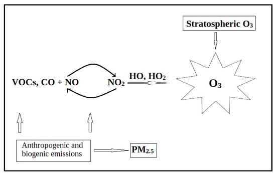
Figure 1.
Formation of ground-level ozone [5].
Tropospheric ozone, with its capacity to oxidize other atmospheric gases, plays a pivotal role in shaping the distribution of trace gases in the troposphere. It is recognized as one of the six major pollutants, notable for its toxicity to ecosystems, human health, and buildings [7,8,9]. While recent attention has been directed towards monitoring suspended particles, particularly PM2.5 and carbon dioxide, it is essential to underscore that atmospheric pollution involving ozone poses a tangible threat to the well-being of ecosystems and individuals. To determine the concentration of ozone in the atmosphere, which is a mixture of many gases, traces of gases, and water vapor, it is necessary to use a very sensitive and selective system. Laser spectroscopy successfully detects specific gases with high sensitivity, providing a fast response. Using infrared-based spectroscopic techniques, such as photoacoustic spectroscopy, molecular gases can be detected at and below the ppb level (part per billion by volume, 1:109). For ultimate performance, optical detection techniques have to operate in the so-called “molecular fingerprint region”. The detection of gases at low concentrations is the strength of laser spectroscopy. Therefore, the detection of pollutants or other trace gases in ambient air is one of the key applications of this technique [10,11,12,13,14].
The primary objective of this study was to evaluate the efficacy of a laser spectroscopy system in accurately quantifying the concentration of O3 within the complex gas mixture present in the ambient air of Magurele, Romania. Additionally, the research sought to examine the influence of meteorological variables on ozone levels. Measurements of ambient air were taken at 1.5 m above the ground. The study was conducted in both the spring and the summer seasons and involved three distinct locations characterized by differences in architectural structure. The laser spectroscopy system served as the analytical tool, offering precise and detailed data on ozone concentrations in the specified locations and seasons.
2. Materials and Methods
2.1. Sampling Sites
The measurements to determine the ozone concentration at ground level were part of a campaign to determine several polluting gases in the ambient air. The campaign took place in the city of Magurele, Romania (44°20′58″ N 26°01′47″ E, 93 m altitude), from March to August 2021 [11]. Magurele serves as a satellite city to the country’s capital, Bucharest. Ozone measurements were realized in three distinct locations, which were chosen to exhibit variability in road configuration and environment characteristics. The location were called P1, P2, and P3 (P1: 44°21′02.7″ N 26°01′42.0″ E; P2: 44°21′10.4″ N 26°02′31.0″ E; P3: 44°22′09.6″ N 26°02′34.2″ E, see Figure 2). Location P1 is situated within the city, nestled in a circuitous path, encompassed by residential structures, and close to both a kindergarten and a primary school. P2 is positioned within a forest, approximately 150 m from the Bucharest city ring road and 100 m from another thoroughfare. P3 is situated in an industrialized zone, adjacent to the road linking the city of Magurele with Bucharest, within an open field.
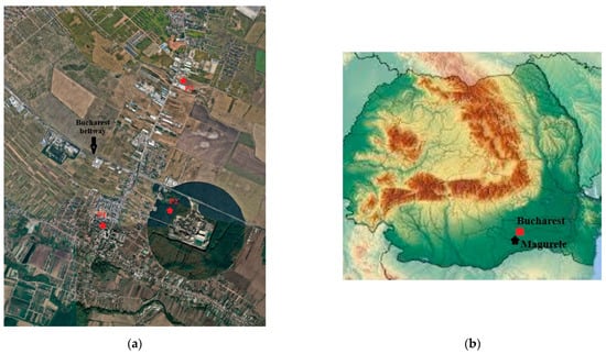
Figure 2.
Air quality monitoring in Magurele. (a) The 3 locations P1, P2, and P3 in Magurele for ozone monitoring; (b) the position of Magurele city on the Romania map.
Ambient air samples were collected at a height of 1.5 m above the ground using specialized containers/bags. Sampling occurred exclusively on working days, Monday through Friday, within the time window from 8:30 am to 8:30 pm. At each location, a total of six samples were collected, with three samples obtained during the morning period between 8:30 and 11:30 am and another three samples collected during the evening period between 5:30 and 8:30 pm. This sampling strategy provided a comprehensive representation of the environmental conditions at different times of the day, allowing for a more thorough analysis of variations in trace gases or other relevant parameters over the day. The dual-sampling timeframes helped capture potential diurnal fluctuations and ensure a more robust understanding of the environmental characteristics at each specific location.
2.2. Methodology
Passive ozone concentration measurements were conducted using a laser-based photoacoustic spectroscopy (LPAS) system. This highly sensitive technique is capable of detecting gas molecules at the ppb level [15,16,17,18]. The LPAS technique offers multiple advantages such as high accuracy and selectivity, a large dynamic range, and the possibility of multicomponent analysis. The scheme of the photoacoustic (PA) detector used in determining the ozone concentration in ambient air is presented in Figure 3. This system comprises a CO2 laser, a PA cell, the detection unit, and a vacuum/gas handling system.
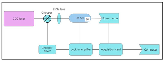
Figure 3.
A schematic representation of the LPAS system employed for determining the ozone concentrations.
The range of wavelengths in which the CO2 laser emitted in the LPAS system was 9.2–10.8 µm, grouped in the 9R, 9P, 10R, and 10P branches, covering 54 different vibrational–rotational lines with a maximum power of 6.5 W. In this range, ozone molecules, in particular, demonstrate significant absorption on the 9P(14) laser line at a wavelength (λ) of 9.5 µm, with an absorption coefficient (α) of 12.7 cm−1atm−1 [19].
In CO2LPAS (CO2 laser photoacoustic spectroscopy), the laser beam was modulated by a mechanical chopper, and a dual-phase lock-in amplifier (Standford Research Systems model SR 830) was employed for signal detection. To address outgassing problems, a stainless-steel PA cell with a volume of 1 dm3 was utilized. The PA cell design, including dimensions (300 mm length and 7 mm inner diameter), acoustic resonator tube, windows, gas inlets/outlets, microphones, and acoustic filter, was optimized to achieve an optimum signal. Therefore, the photoacoustic signal could be obtained at a given frequency, which in this case was 564 Hz, as follows:
where V (V)—photoacoustic signal; α (cm−1 atm−1)—absorption coefficient; C (Pa cm W−1)—cell constant; SM (VPa−1)—microphone sensitivity; PL (W)—laser; and c (atm)—gas concentration.
Equation (1) suggests that the photoacoustic signal exhibits a linear dependence on the laser power. Additionally, the signal is directly proportional to the quantity of molecules within the optical path, serving as an indicator of gas concentration. Consequently, employing this method yields no signal generation in the absence of the target molecules within a sample gas mixture, signifying a “zero-base” approach. At a signal-to-noise ratio SNR = 1, a minimum measurable signal V = Vmin is obtained, and the minimum concentration that can be detected by our photoacoustic system c = cmin is:
The sensitivity of the LPAS system is susceptible to various types of noises, including: electrical noise; this noise is related to random fluctuations, whether electronic or acoustic. To mitigate the electrical noise, a lock-in amplifier set at a detection bandwidth of 0.25 Hz (1 s time constant) was employed in all measurements. The measured electrical noise () was reduced to 0.15 μV/√Hz; coherent acoustic background noise; this noise can arise due to laser beam modulation. The LPAS system effectively addressed this type of noise during the measurements; coherent background signal arising from the heating of the photoacoustic (PA) cell’s windows and walls, attributed to the reflection or scattering of light. This is frequently triggered by imperfections in the focusing lens, windows, or internal cell walls.
All these noises were measured with the LPAS system at the resonance frequency and atmospheric pressure. The electrical noise was , and the acoustic background noise was A background signal was also detected when the photoacoustic cell was filled with pure nitrogen of 99.9999% purity, or 9.6 × 10⁻⁵ Pa/W.
The acoustic waves were detected using four microphones, each with a sensitivity of 20 mV/Pa, mounted flush with the wall. The PA cell was characterized by a quality factor (Q) of 16.1, a cell constant C of 4375 Pacm/W, and a responsivity R of 350 cmV/W, representing its sensitivity to pressure changes. The CO2LPAS system is employed for multicomponent analysis within the CO2 laser spectral range. Water vapor and carbon dioxide fall into the category of absorbent interference from the atmosphere. To mitigate the interference from carbon dioxide and water vapor and enhance the precision of the photoacoustic (PA) signal, we integrated an enclosure with a potassium hydroxide (KOH) scrubber between the sampling cell and the PA cell [20]. Following each measurement, a thorough washing cycle with nitrogen 6.0 (purity 99.9999%) was conducted to uphold the measurement quality (given nitrogen transparency to CO2 laser radiation). The background signal was measured post-cleaning, with effective cleaning indicated by a signal of a maximum of 35 µV (see Figure 4).
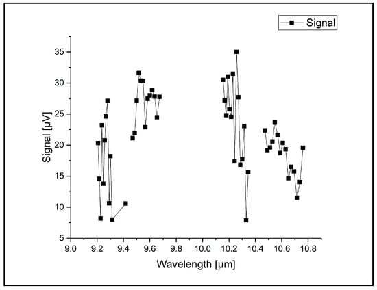
Figure 4.
The absorption spectra of CO2 laser radiation in pure nitrogen 6.0.
Air samples were gathered in specialized aluminum-coated bags and subsequently introduced into the PA cell at a regulated flow rate by the gas handling system. This system serves multiple functions, including monitoring both the total and the partial pressures of gas mixtures, as well as evacuating the gas sample from the cell.
2.3. Meteorological Data
Meteorological variables, encompassing air temperature, relative humidity, atmospheric pressure, wind speed, and direction, were gauged employing a Eurochron WS1080 meteorological station model. The external sensors utilized in the measurements wirelessly transmitted the collected data to the central unit for further analysis and monitoring.
3. Results
In the campaign to assess atmospheric ozone concentrations utilizing a laser spectroscopy-based system, the measurements revealed levels on the order of ppb. During this timeframe, the lowest ozone concentration was identified at the P2 location, corresponding to 7 ppb. Conversely, the peak of ozone level was recorded at the P3 location, reaching 185.5 ppb. Thus, during the entire period of measurement, the average value of ozone concentration was 24.45 ± 16.44 ppb in point P1, 11.96 ± 3.80 ppb in P2, and 95.01 ± 37.11 ppb in point P3. The mean ozone concentration values from March to August in the three measuring points are presented in Figure 5.
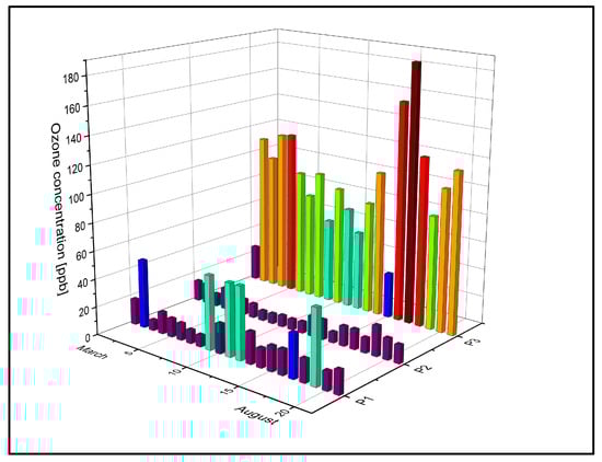
Figure 5.
The dispersion of the mean weekly ozone concentrations in P1, P2, and P3 from March to August 2021 with the highest values indicated by the brown color, followed by the ozone values with red, orange, and green. Values close to background ozone values are indicated in purple.
According to the European Union (EU), the ground-level ozone concentration should be 120 µg/m3 (≅61 ppb) [21] as the daily maximum 8 h mean, while the World Health Organization (WHO) recommends a maximum of 100 µg/m3 (≅51 ppb) [22]. To have an overview of the frequency of the ozone concentration values throughout the measurement period, their dispersion in the three points P1, P2, and P3 was examined, as shown in Figure 6. In this figure, it can be seen that approximately 48% of the determined ozone values exceeded the limit value of 51 ppb. To investigate and identify the meteorological factors impacting ozone production from the surrounding air, we examined a temporal and seasonal model of ozone levels. In our scenario, temperature emerged as a key influencer of ozone levels, as illustrated by the concentration values depicted in Figure 7 monthly.
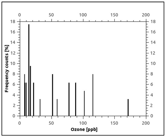
Figure 6.
Frequency ozone concentration values distribution during March–August 2021.
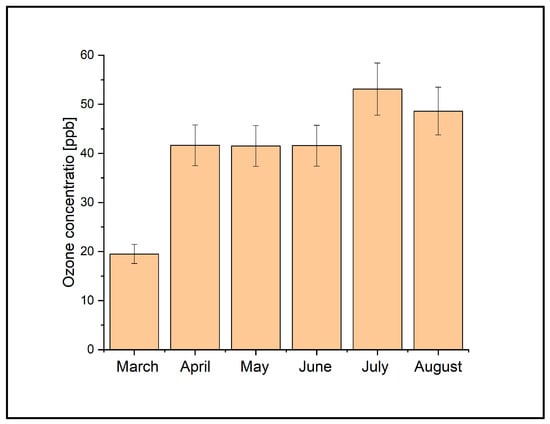
Figure 7.
The average monthly concentrations in the three ozone measurement locations during March–August 2021.
During the six-month period presented in Figure 7, the concentrations of ozone varied, with the highest ozone values measured in July and August, and the peak in July. The observed variations in the mean weekly ozone concentrations could be attributed to the elevated temperatures recorded during the summer of 2021. In Magurele, this period was marked by hot days, with maximum temperatures ranging between 31 °C and 40 °C, tropical nights in July and August, and an exceptionally limited rainfall regime. The temperature variations from March to August in Magurele are presented in Figure 8.
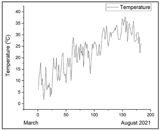
Figure 8.
The variation of the maximum daily temperature in the period March–August 2021.
The ozone concentrations exhibited variation during two distinct time intervals: the first part of the day (8:30–11:30 am) and the second part (5:30–8:30 pm), as depicted in Figure 9. The objective of our analysis was to juxtapose the ozone levels between the early morning and the evening periods. This comparative assessment aimed to ascertain whether ozone production was influenced by photochemical reactions in the surrounding air, under the combined influence of temperature and solar radiation.
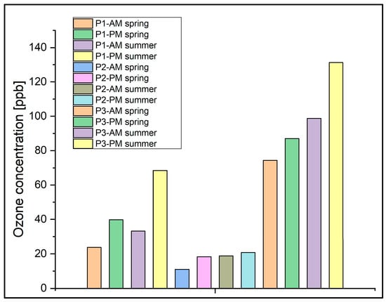
Figure 9.
The diurnal variation of the average ozone concentrations from March to August 2021, in the intervals 08:30–11:30 am and 05:30–08:30 pm at the P1, P2, and P3 locations.
Observing Figure 10 reveals a correlation between ozone concentrations and wind direction, specifically, correlations with wind from the east (E) and northeast (NE) within the range of 54 to 91.5 degrees, as well as from the south (S) and southwest (SV) within the range of 180 to 273.9 degrees. Figure 11 shows the distribution of the ozone concentrations in the P1, P2, and P3 points as a function of wind speed. In this figure, it can be seen that it seems that part of the ozone concentrations were distributed in the range of 2.5–4 m/s.
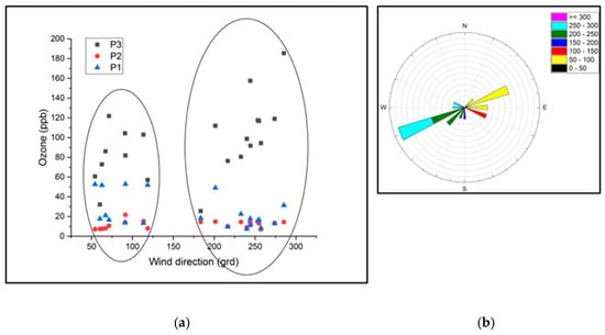
Figure 10.
(a) The distribution of the ozone concentrations in the three measurement locations according to the wind direction; (b) representation of the wind direction in the March–August 2021 period.
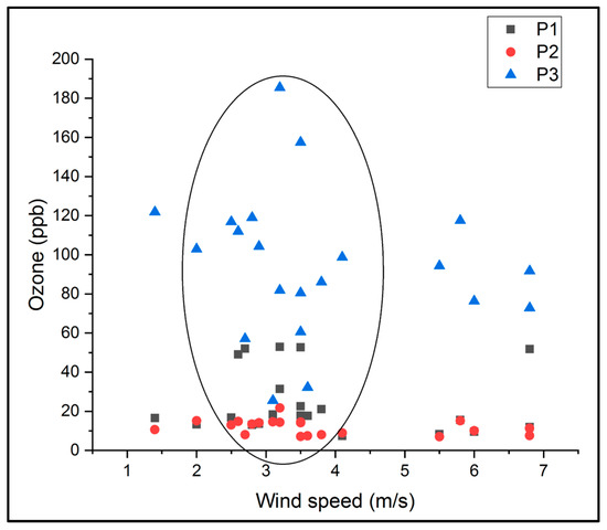
Figure 11.
The distribution of the ozone concentrations in the three measurement locations according to the wind speed.
The results obtained indicated that environmental conditions, including landforms and the area surrounding the monitoring LPAS, exerted a notable influence on the ozone values.
Based on the statistical analyses, our technique identified where the ozone limit levels were exceeded (8 h maximum daily average ≥120.4 μg/m3). According to regulatory standards, there was an exceedance of the ozone limit, accounting for approximately 48% of occurrences in the year 2021. When we evaluated the period March–August 2021 using statistical analyses, we observed that the ozone limit was exceeded in July, while when we evaluated by statistical analyses the zones P1, P2, and P3, we observed that the target level of ozone was exceeded in the P3 zone. With the help of the gas concentration measurement system based on laser photoacoustic spectroscopy, the ozone concentrations at ground level were determined, thereby also determining ozone values that exceed the imposed limits.
4. Discussion
In this investigation, laser spectroscopy was utilized to determine ozone concentrations in ambient air. While sensors are commonly employed for detecting ozone levels, they pose challenges as they may be inaccurate in detecting low ozone levels and are sensitive to humidity changes [23,24,25]. Notably, a study conducted by Anthony Puga et al. in 2023 enhanced ozone measurement parameters using a cavity-enhanced absorption spectroscopic instrument, leveraging the deep-ultraviolet output of a broadband laser-driven light source [26]. While various methods, such as optical, gas chromatographic, and mass spectrometric techniques, have proven effective in detecting environmental trace gases [13], laser spectroscopy has emerged as a promising and successful alternative. In comparison with other ozone detection instruments [27,28,29,30,31,32], the LPAS instruments demonstrated a distinctive advantage. They operate over a broader spectral region, mitigating interference effects from other absorbing species like water [20]. This characteristic makes the LPAS system well suited for applications requiring the detection of various species such as benzene, toluene, methanol, carbon dioxide, acrolein, acetonitrile, and ammonia, among others, where alternative instruments may be less readily available [33]. Although it is acknowledged that instruments with superior parameters exist, their selection depends on the specific application details [17].
In our study, we specifically measured ozone concentrations at a height of 1.5 m above ground level, a significant level that corresponds to the breathing zone for both children and adults. This measurement is essential because ozone exhibits low solubility in water. Once inhaled through the upper respiratory tract, it cannot be easily cleansed and instead reaches the lower respiratory tract, including the lungs. Upon reaching the lungs, ozone undergoes reactions with proteins and lipids present in fluids, triggering lung inflammation [10]. This underscores the importance of monitoring ozone concentrations at the breathing level to better understand and address its potential health impacts, particularly the inflammatory responses in the respiratory system associated with elevated ozone exposure. Ozone, a significant toxic air pollutant at ground level in the troposphere, coexists with background ozone, which is present at concentrations ranging from 10 to 20 ppb [5]. In the P2 point, the ozone levels were in the 7–21.10 ppb range. These low levels of ozone were due to the presence of trees that reduce the level of pollutants in the atmosphere, having a protective role for humans [34]. In the P1 point, the ozone concentrations varied from 7.35 ppb to 52.92 ppb. This point is situated inside the city, surrounded by residential buildings, very close to a primary school and a kindergarten. In the summer season, on days with high temperatures, the ozone concentration values were higher, very close to the limit imposed by the WHO of 51 ppb. The studied location is positioned in an area characterized by a high traffic density, featuring buildings of varying shapes and heights ranging from one to three levels. Despite occasional spikes in ozone concentrations, the overall mean concentration remained low, closely resembling the background ozone level. The street morphology in these areas plays a crucial role in influencing the volume of air in which pollutants emitted by road traffic are dispersed. As Martin and Adnes highlighted, the dispersion of pollutants in urban environments is significantly impacted by the interplay of buildings with diverse shapes and heights along with the layout of roads [35]. If the surrounding buildings are low, then there is a higher potential for air dispersion and dilution. At the P3 location, situated in an industrial area, the ozone concentrations ranged from 25.55 ppb to 185.50 ppb. In both P1 and P3, the highest ozone concentrations were observed on days characterized by elevated temperatures.
Ground-level ozone is produced through a photochemical reaction accelerated by sunlight, particularly in the absence of wind or rain to disperse the air pollution. This reaction involves the combination of two primary pollutants, NOxs and VOCs. These pollutants are commonly emitted from various sources, including industrial plants, electric utilities, vehicle exhaust, wildfire smoke, and activities related to oil and gas extraction. The interaction of NOxs and VOCs in the presence of sunlight leads to the formation of ground-level ozone, a key component of smog. In the cities, ozone formation and destruction are complex processes and depend on solar radiation and pollutant emissions from traffic. According to other studies, the ozone concentrations at the ground level present seasonal, episodic, and diurnal fluctuations [36,37,38,39]. Zhang et al., in their study, highlighted that the ozone concentrations tended to rise during periods of elevated temperatures in the northeastern United States [40]. Their findings indicated that during the summer season, as much as 84% of the variation in long-term peak ozone concentrations could be attributed to changes in seasonal maximum average daily temperature and seasonal average wind speed. Additionally, they noted that approximately 70% of the short-term variation in ozone concentrations was influenced by the maximum daily temperature and the average daily wind speed. This underscores the significant impact of temperature and wind conditions on ozone levels in this region. This relationship between ozone concentration and meteorological variables was also observed in our measurements, where the highest ozone concentrations were determined in the days of July and August when the air temperature reached and even exceeded 40 °C, with tropical nights and low wind speeds between 2 m/s and 4 m/s. According to several studies, solar radiation and temperature play a very important role in the chemical reactions that lead to the formation of ozone in the atmosphere, having a positive correlation with ozone concentrations [41,42,43,44,45]. Indeed, some studies demonstrated that the production of ozone in the environment can increase with rising ambient temperatures even in cases where the concentrations of VOCs or NOxs remain unchanged [46,47]; if the episodes of high temperatures are accompanied by low winds that lead to the stagnation of air at the ground level, an increase in the concentration of ozone will occur [48]. So, ozone concentration depends not only on the concentrations of its precursors but also on certain meteorological variables such as elevated temperature, low wind speed, wind direction, solar radiation, and the period during which a heat wave persists [49,50].
From our ozone measurements, a high ozone concentration was found in the P3 point. A significant influence on ozone concentration was observed to be exerted by the wind speed, with a high wind speed associated with a low ozone concentration in ambient air. The wind direction is an important variable of pollutant dispersion [51]. Wind speed and direction represent meteorological factors that impact the concentration of ground-level ozone, as indicated by our measurements. Bucharest is home to numerous power plants, predominantly fossil fuel-based, which serve as significant contributors to particulate air pollution [52]. The Romanian Ministry of Environment reported that the total annual fuel consumption per power plant consists of 93.59% of natural gas, 6.4% of fuel oil, and 0.01% of diesel fuel [53]. Also, in the afternoon hours, there were big differences in ozone concentrations compared to the first part of the day in all three locations in the spring and summer seasons. This difference is consistent with the appearance of the most intense photochemical processes in the second part of the day under the influence of solar radiation and temperature [2].
The formation of O3 is acknowledged to be contingent on both sources and precursors, as well as the chemical composition of the surrounding air. The chemical pathway leading to the creation of tropospheric ozone commences with solar radiation catalyzing the photo-dissociation of NO2. The ensuing oxygen atoms subsequently engage with the hydrocarbons present in ambient air, giving rise to the formation of ozone. Therefore, the observed fluctuation in ozone concentration, with higher levels noted in the latter part of the day, is attributed to the photochemical process [54].
As was mentioned above, the ozone level limit recommended by the EU is 61 ppb, and that indicated by the WHO is 51 ppb. Thus, in location P3, the ozone concentrations far exceeded the limits imposed by the WHO and the EU, especially in the summer season.
5. Conclusions
This study revealed the results of measuring ambient air ozone concentrations at 1.5 m above the ground in three distinct areas with different architectural structures, utilizing a CO2LPAS detector. The ozone levels showed a robust positive correlation with meteorological variables and key human activities like road traffic and industry. The findings indicated that the air quality standard was exceeded in the developing industrial area, which is also undergoing residential expansion. The industrial zone recorded the highest ozone concentrations, especially during the summer season. Meteorological variables, such as increased solar radiation in the afternoon, contributed to higher concentrations during summer compared to spring. Additionally, the wind direction and speed played a role in altering the ambient air composition. Remarkably, the forested area consistently exhibited the lowest ozone concentrations, underscoring the remarkable pollution-reducing capacity of trees, despite heavy traffic within it.
This study emphasizes the intricate interplay between ozone levels, meteorological conditions, and human activities, shedding light on critical considerations for air quality management in the studied suburban setting. The objective of this study was to model the climate within a small, yet highly significant, region, acknowledging the potential presence of uncertainties in the projections. Various statistical approaches and combinations of meteorological variables were explored. Future research should delve into dissecting the distinct roles of climate change and variability on ozone levels. This is crucial for a more comprehensive understanding of how climate influences surface ozone pollution.
Author Contributions
Conceptualization, M.P.; methodology, M.P., C.P. and A.-M.B.; software, M.P.; validation, M.P., C.P. and A.-M.B.; formal analysis, M.P.; investigation, M.P.; data curation, M.P.; writing—original draft preparation, M.P.; writing—review and editing, M.P., C.P. and A.-M.B.; visualization, M.P.; supervision, M.P., C.P. and A.-M.B.; project administration, M.P. All authors have read and agreed to the published version of the manuscript.
Funding
This research was funded by a grant from the Ministry of Research, Innovation, and Digitization, CNCS-UEFISCDI, project TE 82/2022, number PN-III-P1-1.1-TE-2021-0717, within PNCDI III, and by the Romanian Ministry of Research, Innovation, and Digitalization under the Romanian National Nucleu Program LAPLAS VII—contract no. 30N/2023.
Data Availability Statement
Data are contained within the article.
Conflicts of Interest
The authors declare no conflicts of interest.
References
- Rubin, M.B. The History of Ozone—The Schonbein Period, 1839–1868. Bull. Hist. Chem. 2001, 26, 40–56. [Google Scholar]
- Martins, E.M.; Nunesa, A.C.L.; Corrêa, S.M. Understanding Ozone Concentrations During Weekdays and Weekends in the Urban Area of the City of Rio de Janeiro. J. Braz. Chem. Soc. 2015, 26, 1967–1975. [Google Scholar] [CrossRef]
- Malashock, D.A.; DeLang, M.N.; Jacob, J.S.; Becker, S.; Serre, M.L.; West, J.J.; Chang, K.L.; Cooper, O.R.; Anenberg, S.C. Estimates of ozone concentrations and attributable mortality in urban, peri-urban and rural areas worldwide in 2019. Environ. Res. Lett. 2022, 17, 054023. [Google Scholar] [CrossRef]
- Sicard, P.; Paoletti, E.; Agathokleous, E.; Araminien, V.; Proietti, C.; Coulibaly, F.; De Marco, A. Ozone weekend effect in cities: Deep insights for urban air pollution control. Environ. Res. 2020, 191, 110193. [Google Scholar] [CrossRef] [PubMed]
- Zhang, J.; Wei, Y.; Fang, Z. Ozone Pollution: A Major Health Hazard Worldwide. Front. Immunol. 2019, 10, 2518. [Google Scholar] [CrossRef] [PubMed]
- Jiang, Y.; Huang, J.; Li, G.; Wang, W.; Wang, K.; Wang, J.; Wei, C.; Li, Y.; Deng, F.; Baccarelli, A.A.; et al. Ozone pollution and hospital admissions for cardiovascular events. Eur. Heart J. 2023, 44, 1622–1632. [Google Scholar] [CrossRef] [PubMed]
- Badura, M.; Batog, P.; Drzeniecka-Osiadacz, A.; Modzel, P. Low- and Medium-Cost Sensors for Tropospheric Ozone Monitoring—Results of an Evaluation Study in Wrocław, Poland. Atmosphere 2022, 13, 542. [Google Scholar] [CrossRef]
- IPCC. Climate Change and Land: An IPCC Special Report on Climate Change, Desertification, Land Degradation, Sustainable Land Management, Food Security, and Greenhouse Gas Fluxes in Terrestrial Ecosystems; Shukla, P.R., Skea, J., Buendia, E.C., Masson-Delmotte, V., Pörtner, H.-O., Roberts, D.C., Zhai, P., Slade, R., Connors, S., van Diemen, R., et al., Eds.; IPCC: Geneva, Switzerland, 2019. [Google Scholar]
- Nowack, P.J.; Abraham, N.L.; Maycock, A.C.; Braesicke, P.; Gregory, J.M.; Joshi, M.M.; Osprey, A.; Pyle, J.A. A large ozone-circulation feedback and its implications for global warming assessments. Nat. Clim. Chang. 2015, 5, 41–45. [Google Scholar] [CrossRef]
- Devlin, R.B.; McDonnell, W.F.; Mann, R.; Becker, S.; House, D.E.; Schreinemachers, D.; Koren, H.S. Exposure of humans to ambient levels of ozone for 6.6 hours causes cellular and biochemical changes in the lung. Am. J. Respir. Cell Mol. Biol. 1991, 4, 72–81. [Google Scholar] [CrossRef]
- Petrus, M.; Popa, C.; Bratu, A.-M. Ammonia Concentration in Ambient Air in a Peri-Urban Area Using a Laser Photoacoustic Spectroscopy Detector. Materials 2022, 15, 3182. [Google Scholar] [CrossRef]
- Xia, J.; Zhu, F.; Bounds, J.; Aluauee, E.; Kolomenskii, A.; Dong, Q.; He, J.; Meadows, C.; Zhang, S.; Schuessler, H. Spectroscopic trace gas detection in air-based gas mixtures: Some methods and applications for breath analysis and environmental monitoring. J. Appl. Phys. 2022, 131, 220901. [Google Scholar] [CrossRef]
- Fiddler, M.N.; Begashaw, I.; Mickens, M.A.; Collingwood, M.S.; Assefa, Z.; Bililign, S. Laser Spectroscopy for Atmospheric and Environmental Sensing. Sensors 2009, 9, 10447–10512. [Google Scholar] [CrossRef] [PubMed]
- Ivascu, I.R.; Matei, C.E.; Patachia, M.; Bratu, A.M.; Dumitras, D.C. Multicomponent detection in photoacoustic spectroscopy applied to pollutants in the environmental air. Rom. Rep. Phys. 2015, 67, 1558–1564. [Google Scholar]
- Popa, C.; Petrus, M.; Bratu, A.M. Effect of Wearing Surgical Face Masks on Gas Detection from Respiration Using Photoacoustic Spectroscopy. Molecules 2022, 27, 3618. [Google Scholar] [CrossRef] [PubMed]
- Dumitras, D.C.; Petrus, M.; Bratu, A.M.; Popa, C. Applications of Near Infrared Photoacoustic Spectroscopy for Analysis of Human Respiration: A Review. Molecules 2020, 25, 1728. [Google Scholar] [CrossRef]
- Bratu, A.-M.; Petrus, M.; Popa, C. Identification of Absorption Spectrum for IED Precursors Using Laser Photoacoustic Spectroscopy. Molecules 2023, 28, 6908. [Google Scholar] [CrossRef] [PubMed]
- Dumitras, D.C.; Dutu, D.C.; Matei, C.; Magureanu, A.; Petrus, M.; Popa, C. Laser photoacoustic spectroscopy: Principles, instrumentation, and characterization. J. Optoelectron. Adv. Mater. 2007, 9, 3655. [Google Scholar]
- Patty, R.R.; Russwurm, G.M.; McClenny, W.A.; Morgan, D.R. CO2 Laser Absorption Coefficients for Determining Ambient Levels of O3, NH3, and C2H4. Appl. Opt. 1974, 13, 2850–2854. [Google Scholar] [CrossRef]
- Bratu, A.M.; Popa, C.; Matei, C.; Banita, S.; Dutu, D.C.A.; Dumitras, D.C. Removal of interfering gases in breath biomarker measurements. J. Optoelectron. Adv. Mater. 2011, 13, 1045–1050. [Google Scholar]
- World Health Organization. Air Quality Guidelines for, Particulate Matter, Ozone, Nitrogen Dioxide and Sulfur Dioxide; Global Update 2005; WHO Regional Office for Europe: Copenhagen, Denmark, 2005. [Google Scholar]
- European Commission Directive 2008/50/EC of the European Parliament and of the Council of 21 May 2008 on Ambient Air Quality and Cleaner Air for Europe. 2008. Available online: https://eur-lex.europa.eu/legal-content/EN/ALL/?uri=CELEX%3A32008L0050 (accessed on 10 December 2021).
- Karagulian, F.; Barbiere, M.; Kotsev, A.; Spinelle, L.; Gerboles, M.; Lagler, F.; Redon, N.; Crunaire, S.; Borowiak, A. Review of the Performance of Low-Cost Sensors for Air Quality Monitoring. Atmosphere 2019, 10, 506. [Google Scholar] [CrossRef]
- Arroyo, P.; Gómez-Suárez, J.; Suárez, J.I.; Lozano, J. Low-Cost Air Quality Measurement System Based on Electrochemical and PM Sensors with Cloud Connection. Sensors 2021, 21, 6228. [Google Scholar] [CrossRef]
- Peterson, P.J.D.; Aujla, A.; Grant, K.H.; Brundle, A.G.; Thompson, M.R.; Hey, J.V.; Leigh, R.J. Practical Use of Metal Oxide Semiconductor Gas Sensors for Measuring Nitrogen Dioxide and Ozone in Urban Environments. Sensors 2017, 17, 1653. [Google Scholar] [CrossRef] [PubMed]
- Puga, A.; Yalin, A. Ozone Detection via Deep-Ultraviolet Cavity-Enhanced Absorption Spectroscopy with a Laser Driven Light Source. Sensors 2023, 23, 4989. [Google Scholar] [CrossRef] [PubMed]
- Lee, J.K.; Christen, A.; Ketler, R.; Nesic, Z. A mobile sensor network to map carbon dioxide emissions in urban environments. Atmos. Meas. Tech. 2017, 10, 645–665. [Google Scholar] [CrossRef]
- Washenfelder, R.A.; Wagner, N.L.; Dube, W.P.; Brown, S.S. Measurement of Atmospheric Ozone by Cavity Ring-down Spectroscopy. Environ. Sci. Technol. 2011, 45, 2938–2944. [Google Scholar] [CrossRef] [PubMed]
- Kalnajs, L.E.; Avallone, L.M. A Novel Lightweight Low-Power Dual-Beam Ozone Photometer Utilizing Solid-State Optoelectronics. J. Atmos. Ocean. Technol. 2010, 27, 869–880. [Google Scholar] [CrossRef]
- Gomez, A.L.; Rosen, E.P. Fast response cavity enhanced ozone monitor. Atmos. Meas. Tech. 2013, 6, 487–494. [Google Scholar] [CrossRef]
- Albertson, J.D.; Harvey, T.; Foderaro, G.; Zhu, P.P.; Zhou, X.C.; Ferrari, S.; Amin, M.S.; Modrak, M.; Brantley, H.; Thoma, E.D. A Mobile Sensing Approach for Regional Surveillance of Fugitive Methane Emissions in Oil and Gas Production. Environ. Sci. Technol. 2016, 50, 2487–2497. [Google Scholar] [CrossRef]
- McHale, L.E.; Martinez, B.; Miller, T.W.; Yalin, A.P. Open-path cavity ring-down methane sensor for mobile monitoring of natural gas emissions. Opt. Express 2019, 27, 20084–20097. [Google Scholar] [CrossRef]
- Thorlabs. LEDs on Metal-Core PCBs Deep UV LEDs (265–340 nm). Available online: https://www.thorlabs.com/newgrouppage9.cfm?objectgroup_id=6071 (accessed on 13 December 2023).
- Montes, C.M.; Demler, H.J.; Li, S.; Martin, D.G.; Ainsworth, E.A. Approaches to investigate crop responses to ozone pollution: From O3 -FACE to satellite-enabled modeling. Plant J. 2022, 109, 432–446. [Google Scholar] [CrossRef]
- Martin, N.; Adnes, C. Ozone spatialization in urban and Hinterland areas. Climatologie 2014, 11, 79–84. [Google Scholar] [CrossRef][Green Version]
- Monks, P.S.; Archibald, A.T.; Colette, A.; Cooper, O.; Coyle, M.; Derwent, R.; Fowler, D.; Granier, C.; Law, K.S.; Stevenson, D.S.; et al. Tropospheric ozone and its precursors from the urban to the global scale from air quality to short-lived climate forcer. Atmos. Chem. Phys. 2015, 15, 8889–8973. [Google Scholar] [CrossRef]
- Khoder, M.I. Diurnal, seasonal and weekdays-weekends variations of ground level ozone concentrations in an urban area in greater Cairo. Environ. Monit. Assess. 2009, 149, 349–362. [Google Scholar] [CrossRef] [PubMed]
- Katragkou, E.; Zanis, P.; Tsikerdekis, A.; Kapsomenakis, J.; Melas, D.; Eskes, H.; Flemming, J.; Huijnen, V.; Inness, A.; Schultz, M.G.; et al. Evaluation of near-surface ozone over Europe from the MACC reanalysis. Geosci. Model. Dev. 2015, 8, 2299–2314. [Google Scholar] [CrossRef]
- Toh, Y.Y.; Fook, L.S.; von Glasow, R. The influence of meteorological factors and biomass burning on surface ozone concentrations at Tanah Rata, Malaysia. Atmos. Environ. 2013, 70, 435–446. [Google Scholar] [CrossRef]
- Zhang, J.; Rao, S.T.; Daggupaty, S.M. Meteorological processes and ozone exceedances in the northeastern United States during the 12–16 July 1995 episode. J. Appl. Meteorol. 1998, 37, 776–789. [Google Scholar] [CrossRef]
- Kleanthous, S.; Vrekoussis, M.; Mihalopoulos, N.; Kalabokas, P.; Lelieveld, J. On the temporal and spatial variation of ozone in Cyprus. Sci. Total Environ. 2014, 476–477, 677–687. [Google Scholar] [CrossRef]
- de Miguel, A.; Mateos, D.; Bilbao, J.; Román, R. Sensitivity analysis of ratio between ultraviolet and total shortwave solar radiation to cloudiness, ozone, aerosols and precipitable water. Atmos. Res. 2011, 102, 136–144. [Google Scholar] [CrossRef]
- Pu, X.; Wang, T.J.; Huang, X.; Melas, D.; Zanis, P.; Papanastasiou, D.K.; Poupkou, A. Enhanced surface ozone during the heat wave of 2013 in Yangtze River Delta region. China. Sci. Total Environ. 2017, 603, 807–816. [Google Scholar] [CrossRef]
- Lu, X.; Zhang, L.; Shen, L. Meteorology and Climate Influences on Tropospheric Ozone: A Review of Natural Sources, Chemistry, and Transport Patterns. Curr. Pollut. Rep. 2019, 5, 238–260. [Google Scholar] [CrossRef]
- Riley, M.L.; Jiang, N.; Duc, H.N.; Azzi, M. Long-Term Trends in Inferred Continental Background Ozone in Eastern Australia. Atmosphere 2023, 14, 1104. [Google Scholar] [CrossRef]
- Coates, J.; Mar, K.A.; Ojha, N.; Butler, T.M. The influence of temperature on ozone production under varying NOx conditions—A modelling study. Atmos. Chem. Phys. 2016, 16, 11601–11615. [Google Scholar]
- Nolte, C.G.; Spero, T.L.; Bowden, J.H.; Sarofim, M.C.; Martinich, J.; Mallard, M.S. Regional Temperature-Ozone Relationships Across the U.S. Under Multiple Climate and Emissions Scenarios. J. Air Waste Manag. Assoc. 2021, 71, 1251–1264. [Google Scholar] [CrossRef] [PubMed]
- Li, K.; Chen, L.; Ying, F.; White, S.J.; Jang, C.; Wu, X.; Gao, X.; Hong, S.; Shen, J.; Azzi, M.; et al. Meteorological and chemical impacts on ozone formation: A case study in Hangzhou, China. Atmos. Res. 2017, 196, 40–52. [Google Scholar] [CrossRef]
- Hunová, I.; Brabec, M.; Malý, M. What Are the Principal Factors Affecting Ambient Ozone Concentrations in Czech Mountain Forests? Front. For. Glob. Chang. 2019, 2, 31. [Google Scholar] [CrossRef]
- Pyrgou, A.; Hadjinicolaou, P.; Santamouris, M. Enhanced near-surface ozone under heatwave conditions in a Mediterranean island. Sci. Rep. 2018, 8, 9191. [Google Scholar] [CrossRef]
- Huang, Y.D.; Hou, R.W.; Liu, Z.Y.; Song, Y.; Cui, P.Y.; Kim, C.N. Effects of Wind Direction on the Airflow and Pollutant Dispersion inside a Long Street Canyon. Aerosol Air Qual. Res. 2019, 19, 1152–1171. [Google Scholar] [CrossRef]
- Marmureanu, L.; Deaconu, L.; Vasilescu, J.; Ajtai, N.; Talianu, C. Combined optoelectronic methods used in the monitoring of SO2 emissions and emissions. Environ. Eng. Manag. J. 2013, 12, 277–282. [Google Scholar]
- Romanian Ministry of Environment. Authorization No. 104/13.02.2013 on Green Gases Emissions. 2019. Available online: http://mmediu.ro/new/wp-content/uploads/2014/10/2014-10-20_Autorizatie_GES_2013-ELCEN_CTE_SUD_rev_iulie_2013.pdf (accessed on 23 November 2021).
- Ihedike, C.; Mooney, J.D.; Fulton, J.; Ling, J. Evaluation of real-time monitored ozone concentration from Abuja, Nigeria. BMC Public Health 2023, 23, 496. [Google Scholar] [CrossRef]
Disclaimer/Publisher’s Note: The statements, opinions and data contained in all publications are solely those of the individual author(s) and contributor(s) and not of MDPI and/or the editor(s). MDPI and/or the editor(s) disclaim responsibility for any injury to people or property resulting from any ideas, methods, instructions or products referred to in the content. |
© 2024 by the authors. Licensee MDPI, Basel, Switzerland. This article is an open access article distributed under the terms and conditions of the Creative Commons Attribution (CC BY) license (https://creativecommons.org/licenses/by/4.0/).