
Assessing the Environmental Impact of Eight Alternative Fuels in International Shipping: A Comparison of Marginal vs. Average Emissions

 ,
,  ,
,  and
and
Abstract
:1. Introduction
2. Background and Literature Review
3. Method
3.1. Goal and Scope
3.2. Computational Strategy
3.3. Monetarisation of Emissions
4. Results
5. Discussion
6. Conclusions
Author Contributions
Funding
Data Availability Statement
Acknowledgments
Conflicts of Interest
Glossary and Abbreviations
| GHG | Greenhouse gas |
| Fuel oil | Oil product that does not reach boiling temperature in the crude distillation unit. |
| HFO | Heavy fuel oil—oil product that does not enter the distillation process in a refinery with a vacuum distillation unit. |
| HSFO | High-sulfur fuel oil. |
| MFO | Medium-sulfur fuel oil |
| LSFO | Low-sulfur fuel oil |
| VLSFO | Very-low-sulfur fuel oil, less than 0.5 wt.% sulfur. |
| ULSFO | Ultra-low-sulfur fuel oil, less than 0.1 wt.% sulfur. |
| MGO | Marine gasoil, less than 0.1 wt.% sulfur. |
| mb/d | Millions of barrels per day |
| LCA | Life-cycle assessment |
| LNG | Liquid natural gas |
| LPG | Liquified petroleum gas |
| IEA | International Energy Agency |
| EIA | U.S. Energy Information Administration |
| IMO | International Maritime Organization |
| aLCA | Attributional Life-Cycle Assessment (based on average data) |
| cLCA | Consequential Life-Cycle Assessment (based on marginal data) |
| RoW | Rest of World (abbreviation in Ecoinvent) |
| GLO | Global (abbreviation in Ecoinvent) |
| RER | Europe (abbreviation in Ecoinvent) |
| ai | Carbon footprint to produce fuel i (typically in kg CO2 eq/kg fuel) |
| bi | Specific fuel consumption of the propulsion combustion (MJ fuel/MJ propulsion) |
| ci | Lower heating value, converting the results from kg fuel to MJ (MJ/kg fuel) |
| dj | Characterization factor for emission type j |
| Aij | Combustion emissions for fuel i and emission type j (g/MJ propulsion) |
| qi | Marginal crude oil demand to produce fuel i (kg crude oil/MJ product) |
| q0 | Marginal crude oil demand for reference fuel (VLSFO) (kg crude oil/MJ product) |
| ap | Environmental impact of producing 1 kg of petroleum and burning it in a refinery. |
Appendix A. Appendix Tables

| Product | Allocation to Final Products (g CO2/MJ) |
|---|---|
| Chemicals | 31.1 |
| LPG | 5.2 |
| Gasoline | 5.5 |
| Kerosine | 6.1 |
| Diesel Fuel | 7.2 |
| Heating oil | 4.7 |
| Marine gasoil | 2.9 |
| heavy fuel oil | −3.7 |
| bitumen | −10.1 |
| petroleum coke | −25.0 |
| lubes and wax | 14.1 |
| sulfur | −1.3 |
| Impact Category | HSFO | VLSFO | MGO | LNG | Biomethane | MeOH (Fossil) | MeOH (Bio) | HVO |
|---|---|---|---|---|---|---|---|---|
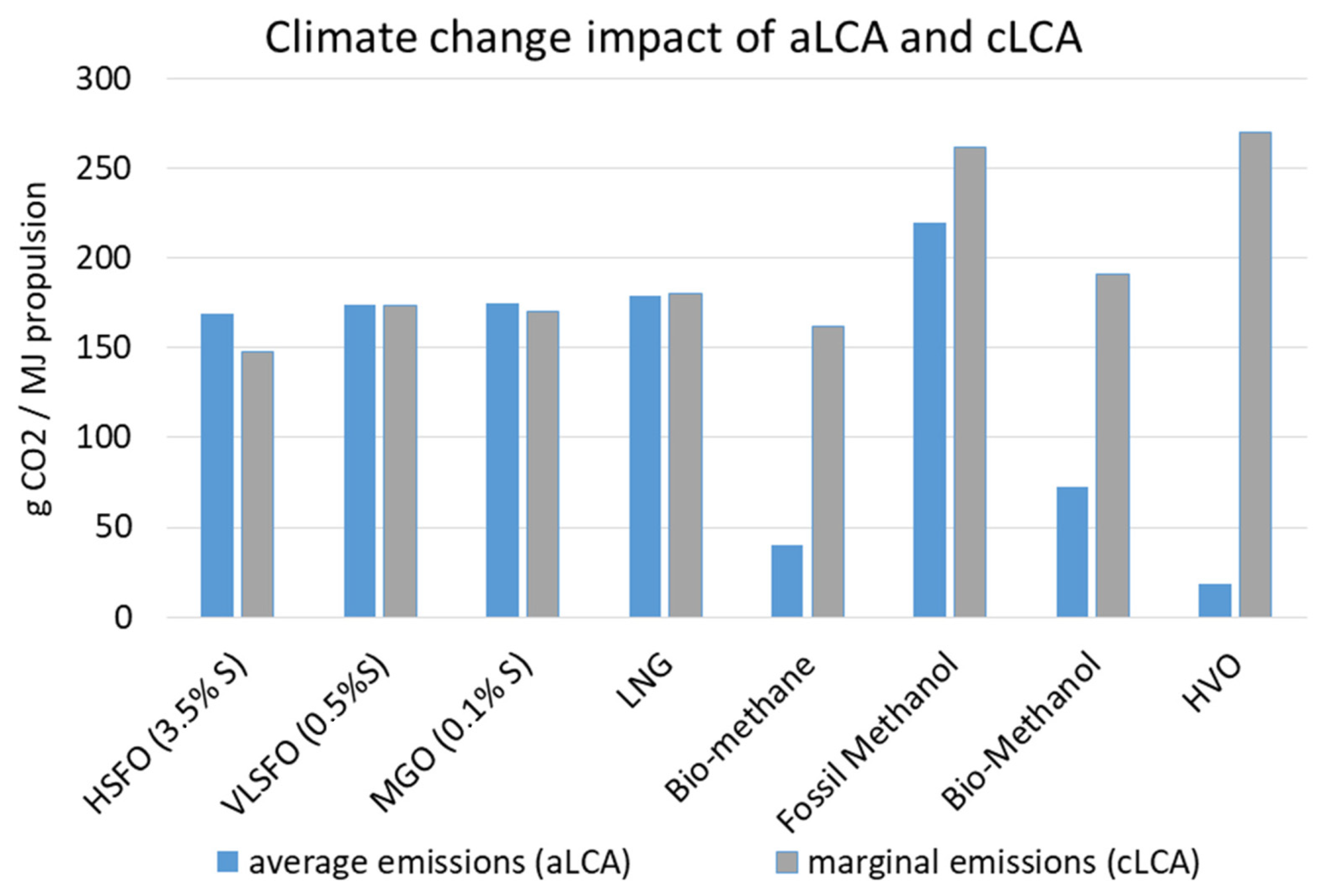
| Climate change (kg CO2 eq) | 1.49 × 10⁻¹ | 1.74 × 10⁻¹ | 1.70 × 10⁻¹ | 1.80 × 10⁻¹ | 1.62 × 10⁻¹ | 2.62 × 10⁻¹ | 1.91 × 10⁻¹ | 2.70 × 10⁻¹ |
| Photochemical ozone formation (kg NMVOC eq) | 4.71 × 10⁻³ | 4.57 × 10⁻³ | 4.27 × 10⁻³ | 4.67 × 10⁻⁴ | 1.13 × 10⁻³ | 1.07 × 10⁻³ | 1.27 × 10⁻³ | 5.49 × 10⁻³ |
| Acidification (mol H+ eq) | 7.55 × 10⁻³ | 4.07 × 10⁻³ | 3.43 × 10⁻³ | 4.34 × 10⁻⁴ | 4.93 × 10⁻⁴ | 7.70 × 10⁻⁴ | 2.07 × 10⁻³ | 4.69 × 10⁻³ |
| Marine eutrophication (kg N eq) | 1.73 × 10⁻³ | 1.74 × 10⁻³ | 1.64 × 10⁻³ | 1.55 × 10⁻⁴ | 5.38 × 10⁻⁴ | 3.60 × 10⁻⁴ | 5.10 × 10⁻⁴ | 2.91 × 10⁻³ |
| Terrestrial eutrophication (kg N eq) | 1.90 × 10⁻² | 1.91 × 10⁻² | 1.79 × 10⁻² | 1.69 × 10⁻³ | 6.87 × 10⁻³ | 3.95 × 10⁻³ | 5.04 × 10⁻³ | 2.39 × 10⁻² |
| Impact Category | HSFO | VLSFO | MGO | LNG | Biomethane | MeOH (Fossil) | MeOH (Bio) | HVO |
|---|---|---|---|---|---|---|---|---|
| Climate change (kg CO2 eq) | 1.69 × 10⁻¹ | 1.74 × 10⁻¹ | 1.75 × 10⁻¹ | 1.80 × 10⁻¹ | 4.01 × 10⁻² | 2.19 × 10⁻¹ | 7.26 × 10⁻² | 1.90 × 10⁻² |
| Photochemical Ozone formation(kg NMVOC eq) | 4.78 × 10⁻³ | 4.57 × 10⁻³ | 4.29 × 10⁻³ | 4.65 × 10⁻⁴ | 3.83 × 10⁻⁴ | 1.09 × 10⁻³ | 1.23 × 10⁻³ | 4.81 × 10⁻³ |
| Acidification (mol H+ eq) | 7.58 × 10⁻³ | 4.10 × 10⁻³ | 3.47 × 10⁻³ | 4.35 × 10⁻⁴ | 3.59 × 10⁻⁴ | 9.15 × 10⁻⁴ | 1.10 × 10⁻³ | 3.70 × 10⁻³ |
| Marine eutrophication (kg N eq) | 1.74 × 10⁻³ | 1.74 × 10⁻³ | 1.64 × 10⁻³ | 1.55 × 10⁻⁴ | 1.43 × 10⁻⁴ | 3.83 × 10⁻⁴ | 4.61 × 10⁻⁴ | 1.87 × 10⁻³ |
| Terrestrial eutrophication (kg N eq) | 1.90 × 10⁻² | 1.90 × 10⁻² | 1.79 × 10⁻² | 1.69 × 10⁻³ | 1.59 × 10⁻³ | 4.18 × 10⁻³ | 4.88 × 10⁻³ | 2.05 × 10⁻² |
| Monetary Cost (EUR/Impact Unit) | ||||
|---|---|---|---|---|
| Environmental Category | Unit | Low | Central | High |
| Climate Change | kg CO2 eq | 0.0615 | 0.1025 | 0.1936 |
| Ozone Depletion | kg CFC-11 eq | 22.8 | 31.4 | 127.2 |
| Ionising radiation, Human health | kBq U235 eq | 0.0008 | 0.0012 | 0.0461 |
| Ozone formation, human health | kg NMVOC eq | 0.87 | 1.19 | 1.9 |
| Particulate matter | Disease incidence | 661,974 | 784,126 | 1,204,600 |
| Human toxicity, non-cancer | CTUh | 30,211 | 163,447 | 755,270 |
| Human toxicity, cancer | CTUh | 174,324 | 902,616 | 2,789,181 |
| Acidification | mol H+ eq | 0.176 | 0.344 | 1.617 |
| Eutrophication, freshwater | kg P eq | 0.26 | 1.92 | 2.18 |
| Eutrophication, marine | kg N eq | 3.21 | 3.21 | 3.21 |
| Ecotoxicity, freshwater | CTUe | 2.39 × 10⁻²⁴ | 3.82 × 10⁻⁵ | 1.88 × 10⁻⁴ |
| Land use (Soil quality index) | dimensionless (pt) | 8.7 × 10⁻⁵ | 0.000175 | 0.000349 |
| Water use | m3 water eq | 0.00419 | 0.00499 | 0.2359 |
| resource use, fossils | MJ | 0 | 0.0013 | 0.0068 |
| Resource use, minerals and metals | kg Sb eq | 0 | 1.64 | 6.53 |
| Environmental Costs EUR per MJ Propulsion | HSFO | VLSFO | MGO | LNG | Bio- Methane | MeOH (Fossil) | MeOH (Bio) | HVO |
|---|---|---|---|---|---|---|---|---|
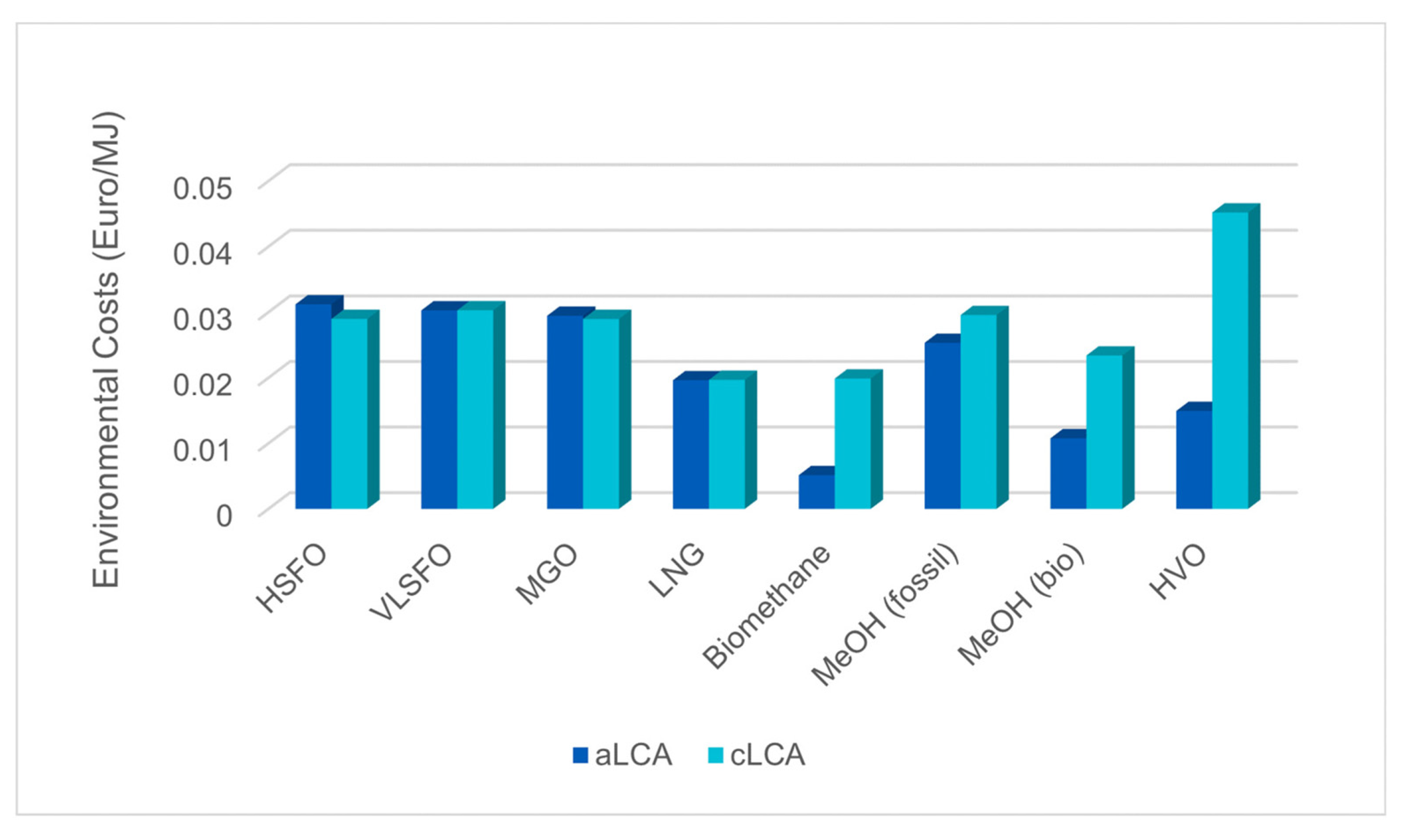
| aLCA | 0.0312 | 0.03028 | 0.02946 | 0.01963 | 0.00515 | 0.02533 | 0.01077 | 0.01494 |
| cLCA | 0.02898 | 0.03029 | 0.02897 | 0.01968 | 0.01988 | 0.02956 | 0.0234 | 0.0452 |
Appendix B. Life-Cycle Inventory
Appendix B.1. Very-Low-Sulfur Fuel Oil (VLSFO)
Appendix B.2. High-Sulfur Fuel Oil (HSFO)
Appendix B.3. Marine Gasoil (MGO)
Appendix B.4. Liquified Natural Gas (LNG)
Appendix B.5. Biomethane (CH4)
Appendix B.6. Methanol (Fossil)
Appendix B.7. Methanol (Biobased)
Appendix B.8. Hydrotreated Vegetable Oil
References
- Vedachalam, S.; Baquerizo, N.; Dalai, A.K. Review on impacts of low sulfur regulations on marine fuels and compliance options. Fuel 2022, 310, 122243. [Google Scholar] [CrossRef]
- Agreement, P. Paris agreement. In Report of the Conference of the Parties to the United Nations Framework Convention on Climate Change (21st Session, 2015: Paris). Retrived December; HeinOnline: Getzville, NY, USA, 2015; p. 2017. [Google Scholar]
- MEPC; IMO. Energy Efficiency of Ships. MEPC 77/6/1 IMO 2021. Available online: https://wwwcdn.imo.org/localresources/en/OurWork/Environment/Documents/Air%20pollution/MEPC%2077-6-1%20-%202020%20report%20of%20fuel%20oil%20consumption%20data%20submitted%20to%20the%20IMO%20Ship%20Fuel%20Oil%20Consumption%20Database%20in%20GISIS.pdf (accessed on 2 May 2023).
- IEA. CO2 Emissions in 2022; IEA Publications: Paris, France, 2023; pp. 1–19. [Google Scholar]
- Xing, H.; Spence, S.; Chen, H. A comprehensive review on countermeasures for CO2 emissions from ships. Renew. Sustain. Energy Rev. 2020, 134, 110222. [Google Scholar] [CrossRef]
- Xing, H.; Stuart, C.; Spence, S.; Chen, H. Alternative fuel options for low carbon maritime transportation: Pathways to 2050. J. Clean. Prod. 2021, 297, 126651. [Google Scholar] [CrossRef]
- IMO. IMO 2020—Cutting Sulphur Oxide Emissions. 2020. Available online: https://www.imo.org/en/MediaCentre/HotTopics/Pages/Sulphur-2020.aspx (accessed on 2 May 2023).
- Krantz, G.; Brandao, M.; Hedenqvist, M.; Nilsson, F. Indirect CO2 emissions caused by the fuel demand switch in international shipping. Transp. Res. Part D Transp. Environ. 2022, 102, 103164. [Google Scholar] [CrossRef]
- Deniz, C.; Zincir, B. Environmental and economical assessment of alternative marine fuels. J. Clean. Prod. 2016, 113, 438–449. [Google Scholar] [CrossRef]
- Zygierewicz, A. Renewable Energy Directive; European Parliamentary Research Service: Brussels, Belgium, 2021. [Google Scholar]
- Gray, N.; McDonagh, S.; O’Shea, R.; Smyth, B.; Murphy, J.D. Decarbonising ships, planes and trucks: An analysis of suitable low-carbon fuels for the maritime, aviation and haulage sectors. Adv. Appl. Energy 2021, 1, 100008. [Google Scholar] [CrossRef]
- EU. Proposal for a Regulation of the European Parliament and of The Council on the Use of Renewable and Low-Carbon Fuels in Maritime Transport and Amending Directive 2009/16/EC; European Commission: Brussels, Belgium, 2021. [Google Scholar]
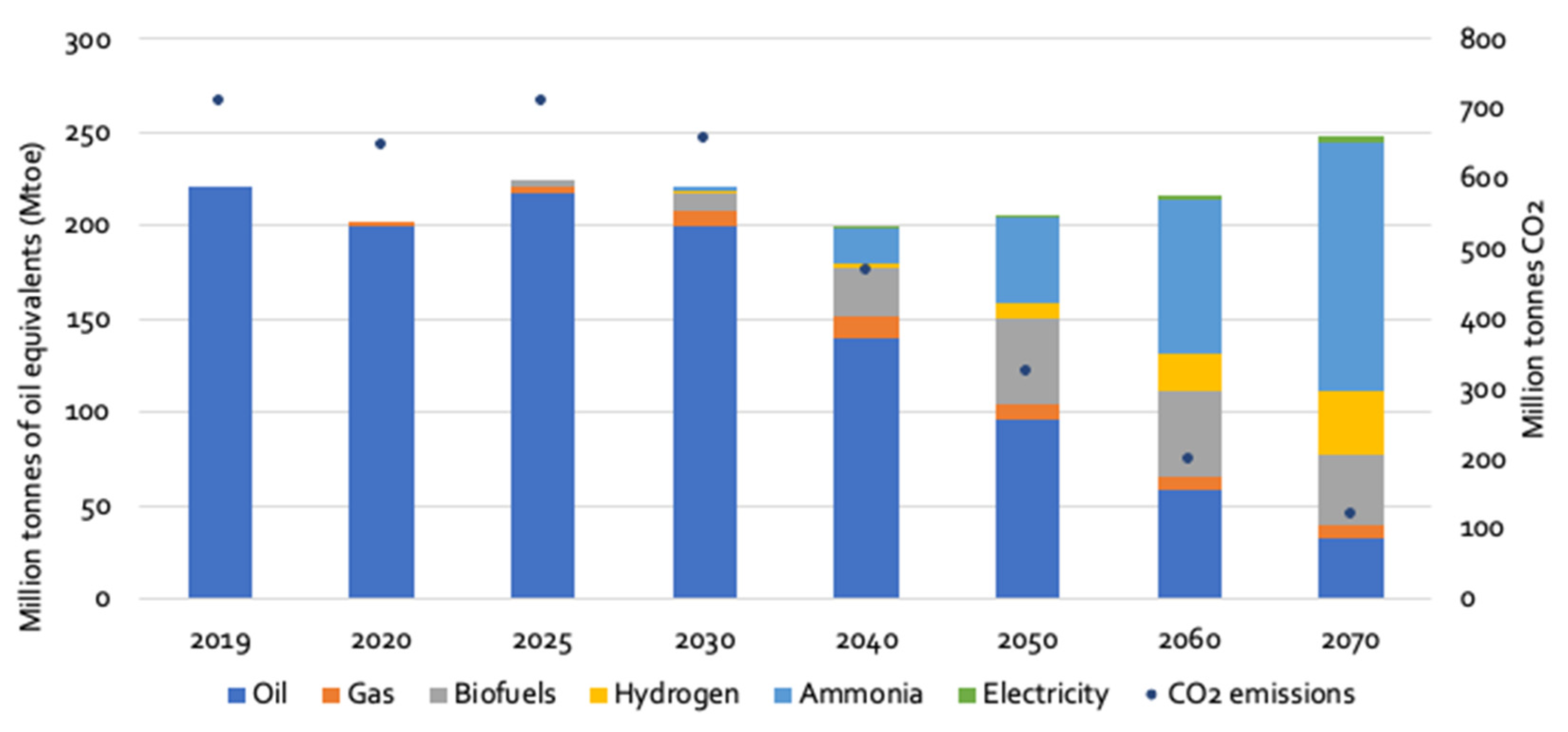
- IEA. Global Energy Consumption and CO2 Emissions in International Shipping in the Sustainable Development Scenario, 2019–2070. Available online: https://www.iea.org/data-and-statistics/charts/global-energy-consumption-and-co2-emissions-in-international-shipping-in-the-sustainable-development-scenario-2019-2070 (accessed on 2 May 2023).
- Andersson, K.; Brynolf, S.; Hansson, J.; Grahn, M. Criteria and decision support for a sustainable choice of alternative marine fuels. Sustainability 2020, 12, 3623. [Google Scholar] [CrossRef]
- Edwards, R.; Padella, M.; Giuntoli, J.; Koeble, R.; O’Connell, A.; Bulgheroni, C.; Marelli, L. Definition of Input Data to Assess GHG Default Emissions from Biofuels in EU Legislation; Version 1c–July 2017; EU Publications: Luxembourg, 2017. [Google Scholar]
- European Union. Directive 2009/28/EC of the European Parliament and of the Council of 23 April 2009 on the promotion of the use of energy from renewable sources and amending and subsequently repealing Directives 2001/77/EC and 2003/30/EC. Off. J. Eur. Union 2009, 5, 2009. [Google Scholar]
- Brynolf, S.; Fridell, E.; Andersson, K. Environmental assessment of marine fuels: Liquefied natural gas, liquefied biogas, methanol and bio-methanol. J. Clean. Prod. 2014, 74, 86–95. [Google Scholar] [CrossRef]
- Bouman, E.A.; Lindstad, E.; Rialland, A.I.; Strømman, A.H. State-of-the-art technologies, measures, and potential for reducing GHG emissions from shipping–A review. Transp. Res. Part D Transp. Environ. 2017, 52, 408–421. [Google Scholar] [CrossRef]
- Balcombe, P.; Brierley, J.; Lewis, C.; Skatvedt, L.; Speirs, J.; Hawkes, A.; Staffell, I. How to decarbonise international shipping: Options for fuels, technologies and policies. Energy Convers. Manag. 2019, 182, 72–88. [Google Scholar] [CrossRef]
- Gilbert, P.; Walsh, C.; Traut, M.; Kesieme, U.; Pazouki, K.; Murphy, A. Assessment of full life-cycle air emissions of alternative shipping fuels. J. Clean. Prod. 2018, 172, 855–866. [Google Scholar] [CrossRef]
- Bilgili, L. Life cycle comparison of marine fuels for IMO 2020 Sulphur Cap. Sci. Total Environ. 2021, 774, 145719. [Google Scholar] [CrossRef]
- Bilgili, L. Comparative assessment of alternative marine fuels in life cycle perspective. Renew. Sustain. Energy Rev. 2021, 144, 110985. [Google Scholar] [CrossRef]
- Al-Douri, A.; Alsuhaibani, A.S.; Moore, M.; Nielsen, R.B.; El-Baz, A.A.; El-Halwagi, M.M. Greenhouse Gases Emissions in Liquified Natural Gas as a Marine Fuel: Life Cycle Analysis and Reduction Potential. Can. J. Chem. Eng. 2022, 100, 1178–1186. [Google Scholar] [CrossRef]
- Comer, B.; O’Malley, J.; Osipova, L.; Pavlenko, N. Comparing the Future Demand for, Supply of, and Life-Cycle Emissions from Bio, Synthetic, and Fossil Lng Marine Fuels in the European Union; ICCT: Washington, DC, USA, 2022. [Google Scholar]
- Jang, H.; Jeong, B.; Zhou, P.; Ha, S.; Nam, D. Demystifying the Lifecycle Environmental Benefits and Harms of Lng as Marine Fuel. Appl. Energy 2021, 292, 116869. [Google Scholar] [CrossRef]
- Livaniou, S.; Chatzistelios, G.; Lyridis, D.V.; Bellos, E. Lng Vs. Mdo in Marine Fuel Emissions Tracking. Sustainability 2022, 14, 3860. [Google Scholar] [CrossRef]
- Winebrake, J.J.; Corbett, J.J.; Umar, F.; Yuska, D. Pollution Tradeoffs for Conventional and Natural Gas-Based Marine Fuels. Sustainability 2019, 11, 2235. [Google Scholar] [CrossRef]
- Burel, F.; Taccani, R.; Zuliani, N. Improving Sustainability of Maritime Transport through Utilization of Liquefied Natural Gas (Lng) for Propulsion. Energy 2013, 57, 412–420. [Google Scholar] [CrossRef]
- Yoo, B.-Y. Economic Assessment of Liquefied Natural Gas (Lng) as a Marine Fuel for CO2 Carriers Compared to Marine Gas Oil (Mgo). Energy 2017, 121, 772–780. [Google Scholar] [CrossRef]
- Paolini, V.; Petracchini, F.; Carnevale, M.; Gallucci, F.; Perilli, M.; Esposito, G.; Segreto, M.; Occulti, L.G.; Scaglione, D.; Ianniello, A. Characterisation and cleaning of biogas from sewage sludge for biomethane production. J. Environ. Manag. 2018, 217, 288–296. [Google Scholar] [CrossRef]
- Ammar, N.R. An Environmental and Economic Analysis of Methanol Fuel for a Cellular Container Ship. Transp. Res. Part D Transp. Environ. 2019, 69, 66–76. [Google Scholar] [CrossRef]
- Oloruntobi, O.; Chuah, L.F.; Mokhtar, K.; Gohari, A.; Onigbara, V.; Chung, J.X.; Mubashir, M.; Asif, S.; Show, P.L.; Han, N. Assessing Methanol Potential as a Cleaner Marine Fuel: An Analysis of Its Implications on Emissions and Regulation Compliance. Clean. Eng. Technol. 2023, 14, 100639. [Google Scholar] [CrossRef]
- Paulauskiene, T.; Bucas, M.; Laukinaite, A. Alternative Fuels for Marine Applications: Biomethanol-Biodiesel-Diesel Blends. Fuel 2019, 248, 161–167. [Google Scholar] [CrossRef]
- Svanberg, M.; Ellis, J.; Lundgren, J.; Landälv, I. Renewable Methanol as a Fuel for the Shipping Industry. Renew. Sustain. Energy Rev. 2018, 94, 1217–1228. [Google Scholar] [CrossRef]
- Shamsul, N.; Kamarudin, S.K.; Rahman, N.; Kofli, N.T. An overview on the production of bio-methanol as potential renewable energy. Renew. Sustain. Energy Rev. 2014, 33, 578–588. [Google Scholar] [CrossRef]
- Issa, M.; Ilinca, A. Petrodiesel and Biodiesel Fuels for Marine Applications. In Petrodiesel Fuels Science, Technology, Health, and Environment; Konur, O., Ed.; Taylor & Francis Group, LLC: Boca Raton, FL, USA, 2021; Volume 3, pp. 1015–1035. [Google Scholar]
- Lin, C.-Y. Effects of biodiesel blend on marine fuel characteristics for marine vessels. Energies 2013, 6, 4945–4955. [Google Scholar] [CrossRef]
- Bicer, Y.; Dincer, I. Environmental impact categories of hydrogen and ammonia driven transoceanic maritime vehicles: A comparative evaluation. Int. J. Hydrog. Energy 2018, 43, 4583–4596. [Google Scholar] [CrossRef]
- Machaj, K.; Kupecki, J.; Malecha, Z.; Morawski, A.; Skrzypkiewicz, M.; Stanclik, M.; Chorowski, M. Ammonia as a potential marine fuel: A review. Energy Strategy Rev. 2022, 44, 100926. [Google Scholar] [CrossRef]
- Wang, X.; Zhu, J.; Han, M. Industrial Development Status and Prospects of the Marine Fuel Cell: A Review. J. Mar. Sci. Eng. 2023, 11, 238. [Google Scholar] [CrossRef]
- Ampah, J.D.; Yusuf, A.A.; Afrane, S.; Jin, C.; Liu, H. Reviewing two decades of cleaner alternative marine fuels: Towards IMO’s decarbonization of the maritime transport sector. J. Clean. Prod. 2021, 320, 128871. [Google Scholar] [CrossRef]
- Bengtsson, S.; Andersson, K.; Fridell, E. Life Cycle Assessment of Marine Fuels: A Comparative Study of Four Fossil Fuels for Marine Propulsion; Chalmers University of Technology: Gothenburg, Sweden, 2011. [Google Scholar]
- Chiong, M.-C.; Kang, H.-S.; Shaharuddin, N.M.R.; Mat, S.; Quen, L.K.; Ten, K.-H.; Ong, M.C. Challenges and opportunities of marine propulsion with alternative fuels. Renew. Sustain. Energy Rev. 2021, 149, 111397. [Google Scholar] [CrossRef]
- El-Houjeiri, H.; Monfort, J.C.; Bouchard, J.; Przesmitzki, S. Life cycle assessment of greenhouse gas emissions from marine fuels: A case study of Saudi crude oil versus natural gas in different global regions. J. Ind. Ecol. 2019, 23, 374–388. [Google Scholar] [CrossRef]
- Elkafas, A.; Rivarolo, M.; Massardo, A. Assessment of alternative marine fuels from environmental, technical, and economic perspectives onboard ultra large container ship. Int. J. Marit. Eng. 2022, 164, 125–134. [Google Scholar] [CrossRef]
- Hansson, J.; Månsson, S.; Brynolf, S.; Grahn, M. Alternative marine fuels: Prospects based on multi-criteria decision analysis involving Swedish stakeholders. Biomass Bioenergy 2019, 126, 159–173. [Google Scholar] [CrossRef]
- Herdzik, J. Decarbonization of marine fuels—The future of shipping. Energies 2021, 14, 4311. [Google Scholar] [CrossRef]
- Horvath, S.; Fasihi, M.; Breyer, C. Techno-economic analysis of a decarbonized shipping sector: Technology suggestions for a fleet in 2030 and 2040. Energy Convers. Manag. 2018, 164, 230–241. [Google Scholar] [CrossRef]
- Huang, J.; Fan, H.; Xu, X.; Liu, Z. Life cycle greenhouse gas emission assessment for using alternative marine fuels: A very large crude carrier (VLCC) case study. J. Mar. Sci. Eng. 2022, 10, 1969. [Google Scholar] [CrossRef]
- Kim, H.; Koo, K.Y.; Joung, T.-H. A study on the necessity of integrated evaluation of alternative marine fuels. J. Int. Marit. Saf. Environ. Aff. Shipp. 2020, 4, 26–31. [Google Scholar] [CrossRef]
- Korczewski, Z. Energy and emission quality ranking of newly produced low-sulphur marine fuels. Pol. Marit. Res. 2022, 29, 77–87. [Google Scholar] [CrossRef]
- Mandić, N.; Ukić Boljat, H.; Kekez, T.; Luttenberger, L.R. Multicriteria analysis of alternative marine fuels in sustainable coastal marine traffic. Appl. Sci. 2021, 11, 2600. [Google Scholar] [CrossRef]
- Moshiul, A.M.; Mohammad, R.; Hira, F.A.; Maarop, N. Alternative marine fuel research advances and future trends: A bibliometric knowledge mapping approach. Sustainability 2022, 14, 4947. [Google Scholar] [CrossRef]
- Prussi, M.; Scarlat, N.; Acciaro, M.; Kosmas, V. Potential and limiting factors in the use of alternative fuels in the European maritime sector. J. Clean. Prod. 2021, 291, 125849. [Google Scholar] [CrossRef]
- Ren, J.; Liang, H. Measuring the sustainability of marine fuels: A fuzzy group multi-criteria decision making approach. Transp. Res. Part D Transp. Environ. 2017, 54, 12–29. [Google Scholar] [CrossRef]
- Rony, Z.I.; Mofijur, M.; Hasan, M.; Rasul, M.; Jahirul, M.; Ahmed, S.F.; Kalam, M.; Badruddin, I.A.; Khan, T.Y.; Show, P.-L. Alternative fuels to reduce greenhouse gas emissions from marine transport and promote UN sustainable development goals. Fuel 2023, 338, 127220. [Google Scholar] [CrossRef]
- Taljegard, M.; Brynolf, S.; Grahn, M.; Andersson, K.; Johnson, H. Cost-effective choices of marine fuels in a carbon-constrained world: Results from a global energy model. Environ. Sci. Technol. 2014, 48, 12986–12993. [Google Scholar] [CrossRef] [PubMed]
- Wang, Y.; Maidment, H.; Boccolini, V.; Wright, L. Life cycle assessment of alternative marine fuels for super yacht. Reg. Stud. Mar. Sci. 2022, 55, 102525. [Google Scholar] [CrossRef]
- Zou, J.; Yang, B. Evaluation of alternative marine fuels from dual perspectives considering multiple vessel sizes. Transp. Res. Part D Transp. Environ. 2023, 115, 103583. [Google Scholar] [CrossRef]
- Abadie, L.M.; Goicoechea, N.; Galarraga, I. Adapting the shipping sector to stricter emissions regulations: Fuel switching or installing a scrubber? Transp. Res. Part D Transp. Environ. 2017, 57, 237–250. [Google Scholar] [CrossRef]
- Ashrafi, M.; Lister, J.; Gillen, D. Toward a harmonization of sustainability criteria for alternative marine fuels. Marit. Transp. Res. 2022, 3, 100052. [Google Scholar] [CrossRef]
- Bilgili, L. A systematic review on the acceptance of alternative marine fuels. Renew. Sustain. Energy Rev. 2023, 182, 113367. [Google Scholar] [CrossRef]
- Corbett, J.J.; Winebrake, J.J. Emissions tradeoffs among alternative marine fuels: Total fuel cycle analysis of residual oil, marine gas oil, and marine diesel oil. J. Air Waste Manag. Assoc. 2008, 58, 538–542. [Google Scholar] [CrossRef] [PubMed]
- Ha, S.; Jeong, B.; Jang, H.; Park, C.; Ku, B. A framework for determining the life cycle GHG emissions of fossil marine fuels in countries reliant on imported energy through maritime transportation: A case study of South Korea. Sci. Total Environ. 2023, 897, 165366. [Google Scholar] [CrossRef]
- Harahap, F.; Nurdiawati, A.; Conti, D.; Leduc, S.; Urban, F. Renewable marine fuel production for decarbonised maritime shipping: Pathways, policy measures and transition dynamics. J. Clean. Prod. 2023, 415, 137906. [Google Scholar] [CrossRef]
- Hermansson, A.L.; Hassellöv, I.-M.; Moldanová, J.; Ytreberg, E. Comparing emissions of polyaromatic hydrocarbons and metals from marine fuels and scrubbers. Transp. Res. Part D Transp. Environ. 2021, 97, 102912. [Google Scholar] [CrossRef]
- Kołakowski, P.; Gil, M.; Wrobel, K.; Ho, Y.-S. State of play in technology and legal framework of alternative marine fuels and renewable energy systems: A bibliometric analysis. Marit. Policy Manag. 2022, 49, 236–260. [Google Scholar] [CrossRef]
- Lindstad, E.; Stokke, T.; Alteskjær, A.; Borgen, H.; Sandaas, I. Ship of the future–A slender dry-bulker with wind assisted propulsion. Marit. Transp. Res. 2022, 3, 100055. [Google Scholar] [CrossRef]
- Merien-Paul, R.H.; Enshaei, H.; Jayasinghe, S.G. In-situ data vs. bottom-up approaches in estimations of marine fuel consumptions and emissions. Transp. Res. Part D Transp. Environ. 2018, 62, 619–632. [Google Scholar] [CrossRef]
- Momenimovahed, A.; Gagné, S.; Gajdosechova, Z.; Corbin, J.C.; Smallwood, G.J.; Mester, Z.; Behrends, B.; Wichmann, V.; Thomson, K.A. Effective density and metals content of particle emissions generated by a diesel engine operating under different marine fuels. J. Aerosol Sci. 2021, 151, 105651. [Google Scholar] [CrossRef]
- Müller-Casseres, E.; Carvalho, F.; Nogueira, T.; Fonte, C.; Império, M.; Poggio, M.; Wei, H.K.; Portugal-Pereira, J.; Rochedo, P.R.; Szklo, A. Production of alternative marine fuels in Brazil: An integrated assessment perspective. Energy 2021, 219, 119444. [Google Scholar] [CrossRef]
- Ni, P.; Wang, X.; Li, H. A review on regulations, current status, effects and reduction strategies of emissions for marine diesel engines. Fuel 2020, 279, 118477. [Google Scholar] [CrossRef]
- Schwartz, H.; Gustafsson, M.; Spohr, J. Emission abatement in shipping–is it possible to reduce carbon dioxide emissions profitably? J. Clean. Prod. 2020, 254, 120069. [Google Scholar] [CrossRef]
- Sofiev, M.; Winebrake, J.J.; Johansson, L.; Carr, E.W.; Prank, M.; Soares, J.; Vira, J.; Kouznetsov, R.; Jalkanen, J.-P.; Corbett, J.J. Cleaner fuels for ships provide public health benefits with climate tradeoffs. Nat. Commun. 2018, 9, 406. [Google Scholar] [CrossRef] [PubMed]
- Van, T.C.; Ramirez, J.; Rainey, T.; Ristovski, Z.; Brown, R.J. Global impacts of recent IMO regulations on marine fuel oil refining processes and ship emissions. Transp. Res. Part D Transp. Environ. 2019, 70, 123–134. [Google Scholar] [CrossRef]
- Winebrake, J.J.; Corbett, J.J.; Meyer, P.E. Energy use and emissions from marine vessels: A total fuel life cycle approach. J. Air Waste Manag. Assoc. 2007, 57, 102–110. [Google Scholar] [CrossRef] [PubMed]
- Winnes, H.; Fridell, E.; Moldanová, J. Effects of marine exhaust gas scrubbers on gas and particle emissions. J. Mar. Sci. Eng. 2020, 8, 299. [Google Scholar] [CrossRef]
- Dang, S.; Yang, H.; Gao, P.; Wang, H.; Li, X.; Wei, W.; Sun, Y. A review of research progress on heterogeneous catalysts for methanol synthesis from carbon dioxide hydrogenation. Catal. Today 2019, 330, 61–75. [Google Scholar] [CrossRef]
- Zetterdahl, M.; Salo, K.; Fridell, E.; Sjöblom, J. Impact of aromatic concentration in marine fuels on particle emissions. J. Mar. Sci. App 2017, 16, 352–361. [Google Scholar] [CrossRef]
- Ecoinvent. Attributional Database. The Ecoinvent Centre, the Swiss Centre for Life Cycle Inventories: Zurich, Switzerland. 2021. Available online: https://ecoinvent.org/the-ecoinvent-database/ (accessed on 2 May 2023).
- Brynolf, S.; Magnusson, M.; Fridell, E.; Andersson, K. Compliance possibilities for the future ECA regulations through the use of abatement technologies or change of fuels. Transp. Res. Part D Transp. Environ. 2014, 28, 6–18. [Google Scholar] [CrossRef]
- Capaz, R.S.; Posada, J.A.; Osseweijer, P.; Seabra, J.E. The carbon footprint of alternative jet fuels produced in Brazil: Exploring different approaches. Resour. Conserv. Recycl. 2021, 166, 105260. [Google Scholar] [CrossRef]
- Schaubroeck, T.; Schaubroeck, S.; Heijungs, R.; Zamagni, A.; Brandão, M.; Benetto, E. Attributional & consequential life cycle assessment: Definitions, conceptual characteristics and modelling restrictions. Sustainability 2021, 13, 7386. [Google Scholar]
- Roos, A.; Ahlgren, S. Consequential life cycle assessment of bioenergy systems—A literature review. J. Clean. Prod. 2018, 189, 358–373. [Google Scholar] [CrossRef]
- Sonnemann, G.; Vigon, B.; Rack, M.; Valdivia, S. Global guidance principles for life cycle assessment databases: Development of training material and other implementation activities on the publication. Int. J. Life Cycle Assess. 2013, 18, 1169–1172. [Google Scholar] [CrossRef]
- Brandão, M.; Azzi, E.; Novaes, R.M.; Cowie, A. The modelling approach determines the carbon footprint of biofuels: The role of LCA in informing decision makers in government and industry. Clean. Environ. Syst. 2021, 2, 100027. [Google Scholar] [CrossRef]
- Moretti, C.; Moro, A.; Edwards, R.; Rocco, M.V.; Colombo, E. Analysis of standard and innovative methods for allocating upstream and refinery GHG emissions to oil products. Appl. Energy 2017, 206, 372–381. [Google Scholar] [CrossRef]
- Ecoinvent. Consequential Database. The Ecoinvent Centre, the Swiss Centre for Life Cycle Inventories: Zurich, Switzerland. 2021. Available online: https://ecoinvent.org/the-ecoinvent-database/ (accessed on 2 May 2023).
- Moretti, C.; Junginger, M.; Shen, L. Environmental life cycle assessment of polypropylene made from used cooking oil. Resour. Conserv. Recycl. 2020, 157, 104750. [Google Scholar] [CrossRef]
- ETIP. European Technology and Innovation Platform Bioenergy (ETIP Bioenergy). ETIP Bioenergy Factsheet: 2020. Available online: https://www.etipbioenergy.eu/fact-sheets (accessed on 2 May 2023).
- Calzado Catalá, F.; De Vuyst, K.; De Meerleer, W.; Gardzinski, W.; Huesken, S.; Iglesias Lopez, A.; Kawula, J.; Lambert, G.; Ludger, M.; Mirabella, W.; et al. Estimating the Marginal CO2 Intensities of EU Refinery Products; CONCAWE Reports: Brussels, Belgium, 2017; Volume 1, pp. 1–28. [Google Scholar]
- Tehrani Nejad M, A. Allocation of CO2 emissions in petroleum refineries to petroleum joint products: A linear programming model for practical application. Energy Econ. 2007, 29, 974–997. [Google Scholar] [CrossRef]
- Amadei, A.M.; De Laurentiis, V.; Sala, S. A review of monetary valuation in life cycle assessment: State of the art and future needs. J. Clean. Prod. 2021, 329, 129668. [Google Scholar] [CrossRef]
- Teuchies, J.; Cox, T.J.; Van Itterbeeck, K.; Meysman, F.J.; Blust, R. The impact of scrubber discharge on the water quality in estuaries and ports. Environ. Sci. Eur. 2020, 32, 103. [Google Scholar] [CrossRef]
- Low Blomberg, E. Scrubber-Fitted Ships See Huge Savings as Fuel Spread Widens. 2022. Available online: https://gcaptain.com/scrubber-fitted-ships-see-huge-savings-as-fuel-spreadwidens/#:~:text=About%208%25%20of%20the%20global,according%20to%20Drewry%20Maritime%20Services (accessed on 2 May 2023).
- Moretti, C.; Vera, I.; Junginger, M.; López-Contreras, A.; Shen, L. Attributional and consequential LCAs of a novel bio-jet fuel from Dutch potato by-products. Sci. Total Environ. 2022, 813, 152505. [Google Scholar] [CrossRef]
- Hönig, V.; Prochazka, P.; Obergruber, M.; Smutka, L.; Kučerová, V. Economic and technological analysis of commercial LNG production in the EU. Energies 2019, 12, 1565. [Google Scholar] [CrossRef]
- Howarth, R.W.; Jacobson, M.Z. How green is blue hydrogen? Energy Sci. Eng. 2021, 9, 1676–1687. [Google Scholar] [CrossRef]
| HSFO | HVO | LNG (Fossil) | LBG | Bio-LNG | Biomethane | Methanol (Fossil) | Methanol (Biobased) | Source |
|---|---|---|---|---|---|---|---|---|
| 84 | - | 56 | 78 | 9 | (EcoInvent 2021) [80] | |||
| 84 | 62 | 27 | 89 | 17 | (Brynolf 2014) [81] | |||
| 94 | 30–700 | 76.5 | 13–17 | 36–46 | (Gray, et al., 2021) [11] | |||
| 86 | 82 | 53 | 92 | (Gilbert, et al., 2018) [20] | ||||
| 100 | 35–45 | 95 | 50 | 19 | 105 | 14 | (Balcombe, et al., 2019) [19] |
| Fuel (and Vector d) | a: (cLCA)kg CO2/kg | a: (aLCA)kg CO2/kg | b: MJ/ MJ | c: MJ/ kg | A: g/MJ Propulsion | ||||
|---|---|---|---|---|---|---|---|---|---|
| CO2 | CH4 | N2O | SOx | NOx | |||||
| HSFO (3.5% S) | 0.336 | 0.332 | 2.01 | 40.5 | 150 | 0.00278 | 0.00750 | 3.14 | 4.39 |
| VLSFO (0.5%S) | 0.463 | 0.459 | 2.01 | 43.1 | 150 | 0.00278 | 0.00750 | 0.449 | 4.39 |
| MGO (0.1% S) | 0.571 | 0.568 | 2.04 | 43.1 | 146 | 0.00278 | 0.00722 | 0.0889 | 4.11 |
| LNG | 0.674 | 0.664 | 1.96 | 39.0 | 114 | 0.833 | 0.00444 | 0.00083 | 0.325 |
| Biomethane | 3.796 | 0.937 | 1.96 | 45.8 | 0 | 0 | 0 | 0 | 0 |
| Fossil Methanol | 1.106 | 0.703 | 2.12 | 20.0 | 145 | 0 | 0 | 0 | 0.847 |
| Biomethanol | 1.801 | 0.686 | 2.12 | 20.0 | 0 | 0 | 0 | 0 | 0 |
| HVO | 5.883 * | 0.387 * | 2.03 | 44.4 | 0 | 0.00178 | 0.00361 | 0.103 | 4.75 |
| … | |||||||||
| d: (kg CO2/g) | 0.001 | 0.0368 | 0.298 | 0 | 0 | ||||
| Environmental Category | Unit | Monetary Cost (EUR/Impact Unit) |
|---|---|---|
| Climate Change | kg CO2 eq | 0.1025 |
| Ozone formation, human health | kg NMVOC eq | 1.19 |
| Acidification | mol H+ eq | 0.344 |
| Eutrophication, marine | kg N eq | 3.21 |
Disclaimer/Publisher’s Note: The statements, opinions and data contained in all publications are solely those of the individual author(s) and contributor(s) and not of MDPI and/or the editor(s). MDPI and/or the editor(s) disclaim responsibility for any injury to people or property resulting from any ideas, methods, instructions or products referred to in the content. |
© 2023 by the authors. Licensee MDPI, Basel, Switzerland. This article is an open access article distributed under the terms and conditions of the Creative Commons Attribution (CC BY) license (https://creativecommons.org/licenses/by/4.0/).
Share and Cite
Krantz, G.; Moretti, C.; Brandão, M.; Hedenqvist, M.; Nilsson, F. Assessing the Environmental Impact of Eight Alternative Fuels in International Shipping: A Comparison of Marginal vs. Average Emissions. Environments 2023, 10, 155. https://doi.org/10.3390/environments10090155
Krantz G, Moretti C, Brandão M, Hedenqvist M, Nilsson F. Assessing the Environmental Impact of Eight Alternative Fuels in International Shipping: A Comparison of Marginal vs. Average Emissions. Environments. 2023; 10(9):155. https://doi.org/10.3390/environments10090155
Chicago/Turabian StyleKrantz, Gustav, Christian Moretti, Miguel Brandão, Mikael Hedenqvist, and Fritjof Nilsson. 2023. "Assessing the Environmental Impact of Eight Alternative Fuels in International Shipping: A Comparison of Marginal vs. Average Emissions" Environments 10, no. 9: 155. https://doi.org/10.3390/environments10090155
APA StyleKrantz, G., Moretti, C., Brandão, M., Hedenqvist, M., & Nilsson, F. (2023). Assessing the Environmental Impact of Eight Alternative Fuels in International Shipping: A Comparison of Marginal vs. Average Emissions. Environments, 10(9), 155. https://doi.org/10.3390/environments10090155