Article

Model Application for Estimation of Agri-Environmental Indicators of Kiwi Production: A Case Study in Northern Greece

Department of Hydraulics, Soil Science and Agricultural Engineering, School of Agriculture, Faculty of Agriculture, Forestry and Natural Environment, Aristotle University of Thessaloniki, 54124 Thessaloniki, Greece
*
Author to whom correspondence should be addressed.
Environments 2023, 10(4), 69; https://doi.org/10.3390/environments10040069
Submission received: 15 March 2023 / Revised: 11 April 2023 / Accepted: 18 April 2023 / Published: 21 April 2023
(This article belongs to the Special Issue Environmental Impact Assessment II)

Abstract

:
Due to the sensitivity of kiwifruit to soil water and nutrient availability, kiwi production is often associated with over-watering and over-fertilization, especially with nitrogen (N), resulting in increased environmental risks. Crop models are powerful tools for simulating crop production and environmental impact of given management practices. In this study, the CropSyst model was applied to estimate soil N budget and environmental effects of kiwi production, with particular regard to N losses, in two grower-managed kiwi orchards in northern Greece, involving two seasons and different management practices. Management options included N fertilization and irrigation. Model estimates were compared with yield and soil mineral N content (0–90 cm depths) measured three times within the growing season. Agri-environmental indicators were calculated based on the N budget simulation results to assess the environmental consequences (focusing on N losses and water use efficiency) of the different management practices in kiwi production. According to model simulation results, kiwifruit yield and N uptake were similar in both orchards. N losses to the environment, however, were estimated on average to be 10.3% higher in the orchard with the higher inputs of irrigation water and N fertilizer. The orchard with the lower inputs showed better water and N use efficiency. N leaching losses were estimated to be higher than 70% of total available soil N in both study sites, indicating potential impact on groundwater quality. These findings demonstrate the necessity for improved irrigation and N fertilization management in kiwi production in the area.

1. Introduction

Kiwi (Actinidia deliciosa (A. chev.) C.F. Liang et A.R. Ferguson var. deliciosa) is a deciduous vine indigenous to the mountainous regions of central and southwestern China. Approximately 85% of the world production of kiwi is from China, New Zealand, Italy, and Greece [1]. The world production of kiwifruit was estimated at 4.4 × 10⁶ Mg in 2020 [1]. The consumption of kiwifruit is increasing each year in central Europe, indicating an expanding market. In Greece, the annual production of kiwi was 256.1 × 10³ Mg in 2019 which corresponds to a production area of 10.4 × 10³ ha [2]. Kiwi orchards are often a monoculture and intensively irrigated, especially in the northern part of Greece. In these areas, farmers have been systematically occupied with kiwi production since the second half of the 20th century. In Greece, the dominant kiwifruit cv. since 1973 has been Hayward. However, selection among 15,000 seedlings originating from open-pollinated ‘Hayward’ plants in northern Greece in 1989 by the farmer Christos Tsechelidis resulted in the cv. Tsechelidis [3]. In the region of Pieria, kiwi production is a dynamic agricultural activity and represents 60% of Greek production with an area covering 3.1 × 10³ ha.
Kiwifruit requires high amounts of irrigation water when cultivated in Mediterranean regions, which are characterized by high light intensities, low precipitation, and relatively high vapor pressure deficits [4]. In these growing conditions, kiwifruit seasonal irrigation volumes can reach about 10–12 × 103 m3 ha−1 [5]. Farmers tend to over-water kiwi since it leads to larger fruits, but this reduces their dry mass and jeopardizes their maintenance after harvest [6]. The risks of over-watering range from groundwater depletion to plant suffocation. In addition, water management has an important effect on kiwifruit production. Evapotranspiration in kiwi orchards increases with increasing levels of water applied and is dependent on water demand, applied water, irrigation method used, canopy cover, and water management. In view of the reduced water availability for the agricultural sector and the foreseen climate change, it is important to develop innovative and more efficient irrigation strategies for optimizing the crop’s irrigation scheduling [7]. Proper irrigation water management in kiwi production will provide high yields of high-quality fruits, having a considerable effect on the orchard’s profitability.
The mineral composition of kiwifruit is an important factor for its quality, in particular its nutritional properties. Adult kiwifruit requires approximately 150 kg Ν ha−1 year−1 [8]. N fertilization is the key factor for obtaining significant fruit yield in terms of quantity and quality and ensuring the economic viability of the orchard. More than half of the global population is fed by crops grown with the use of synthetic N fertilizers [9]. However, only about half of the N fertilizer applied to soil is typically consumed by crops, while the other half either remains in soil or is lost from fields into the water and atmosphere [10,11], posing health, environmental, and economic problems [12]. Excessive application of N fertilizer in relation to crop N requirements can negatively impact fruit quality after harvest and during storage and results in large amounts of residual nitrate N in soil [13] which can be easily leached into deep soil layers, causing substantial negative environmental impacts [14].
N losses to the environment from agricultural activities constitute one of the prime polluting factors potentially resulting in severe environmental impact through greenhouse gas emissions (nitrous oxide and ammonia) to the atmosphere and losses of nitrate and organic N compounds to water bodies [12,15]. Agri-environmental indicators are considered a useful tool to assess the sustainability of different agricultural management systems [15,16]. Although combining soil testing, N fertilizer experiences of the farmer, and projected crop N requirement (expected yield) is a good method for determining N fertilizer application rates [17], it is rather difficult to manage the fate of N in cropping systems aiming to maintain yield increases with the world’s limited land resources [18,19]. Increased yields require a larger pool of plant-available soil N to increase crop growth, but this is more prone to N losses from volatilization, denitrification, and leaching [18]. According to Müller et al. [20], carbon footprints of kiwifruit orchards could be decreased by more accurately adjusting fertilization to crop requirements by monitoring and accounting for plant-available soil N. The plant-available soil N pool, however, is rather difficult to predict and manage [18,19].
Crop growth simulation models have been widely applied for optimizing water and N management in agriculture [21] and are powerful tools in providing information regarding the ability of given management practices to increase productivity while minimizing the environmental impact [22,23,24] for increasing the agroecosystem efficiency. The simulation of crop growth is based on a complex interaction between weather parameters, soil properties, plant characteristics, and management practices which influence crop response to various water and nutrient inputs [25]. The use of crop growth models in agriculture favors the management of water and nutrient resources and supports comparing different management scenarios that aim at the reduction of non-beneficial resource uses and the increase in crop productivity and economic farm revenue [26]. An increasing number of models have been adapted for specific purposes and scales of application using different input variables and crop growth engines [27,28,29].
In spite of the large number of studies on model calibration and validation regarding crop growth and development, there are few papers in the literature about the evaluation of crop models for simulating water and nutrient dynamics. The CropSyst model was evaluated for simulating the N balance in field experiments carried out in northern Italy between 2002 and 2004 [30]. The results showed the robustness of the model in reproducing the course of the measured soil mineral N content and the same level of reliability while simulating the N balances under different levels of N fertilization, thus depicting it as suitable for comparing N fertilization scenarios. In a study conducted by Tahir et al. [31] where the Agricultural Production System Simulator (APSIM) model [32,33] was used to simulate soil N in black soil in China for 20 years, the observed values were consistent with the simulated values of N dynamics, denitrification, and N losses through different soil depths. A field experiment was carried out in New Delhi [34] to quantify the N dynamics in rice crops using the InfoCrop model. Simulated results matched well with the observed values in terms of yield of rice and seasonal N uptake with the components of soil N balance (denitrification, volatilization, N2O emissions) differing among varying N level treatments.
The Cropping Systems (CropSyst) simulation model [35] is a multi-year multi-crop simulation model developed to study the effect of cropping systems management on productivity and environment and has been used to simulate the growth of several crops with generally good results in many parts of the world [36]. The model appears a promising tool for analyzing management practices regarding water and nitrogen [22]. CropSyst was developed with a focus on crop processes and has fundamental differences from approaches adopted by other models such as the Erosion–Productivity Impact Calculator (EPIC) [37] which was originally developed for erosion prediction but has also been applied for cropping systems analysis. Moreover, the water budget in CropSyst shows distinctive features not found in other management-oriented crop growth models. The simple approach of nitrogen transport in CropSyst is preferable compared to models such as the LEACHM model [38] which is more complex with greater input data requirements and longer execution time. Hence, the use of the CropSyst model can lead to a better understanding of the crop response under different environmental conditions and management practices in agriculture.
This paper investigates the effects on soil N dynamics of irrigation and N fertilizer practices, in two grower-managed kiwi orchards in the area of Pieria in northern Greece. The research aim was to set up a crop model to compare the effects on the environment, with particular regard to N losses and water use efficiency of local current management practices in kiwi production. The CropSyst model was used to simulate crop yield and N budget. Model estimates were compared with field data of yield and soil mineral N content (0–90 cm depths) measured three times within the growing season, for two consecutive years. The specific objectives of the study were (1) to estimate the effects of irrigation and N fertilization management practices on N budget using the CropSyst model and (2) to evaluate the potential environmental impact of the different management practices using agri-environmental indicators. To the best of our knowledge, there is limited published research on environmental assessment of kiwi production in the wider area of northern Greece, where the majority of Greek kiwi production takes place. This paper adds knowledge to the research on environmental consequences of the production of kiwi, a non-traditional crop in the Mediterranean region.

2. Materials and Methods

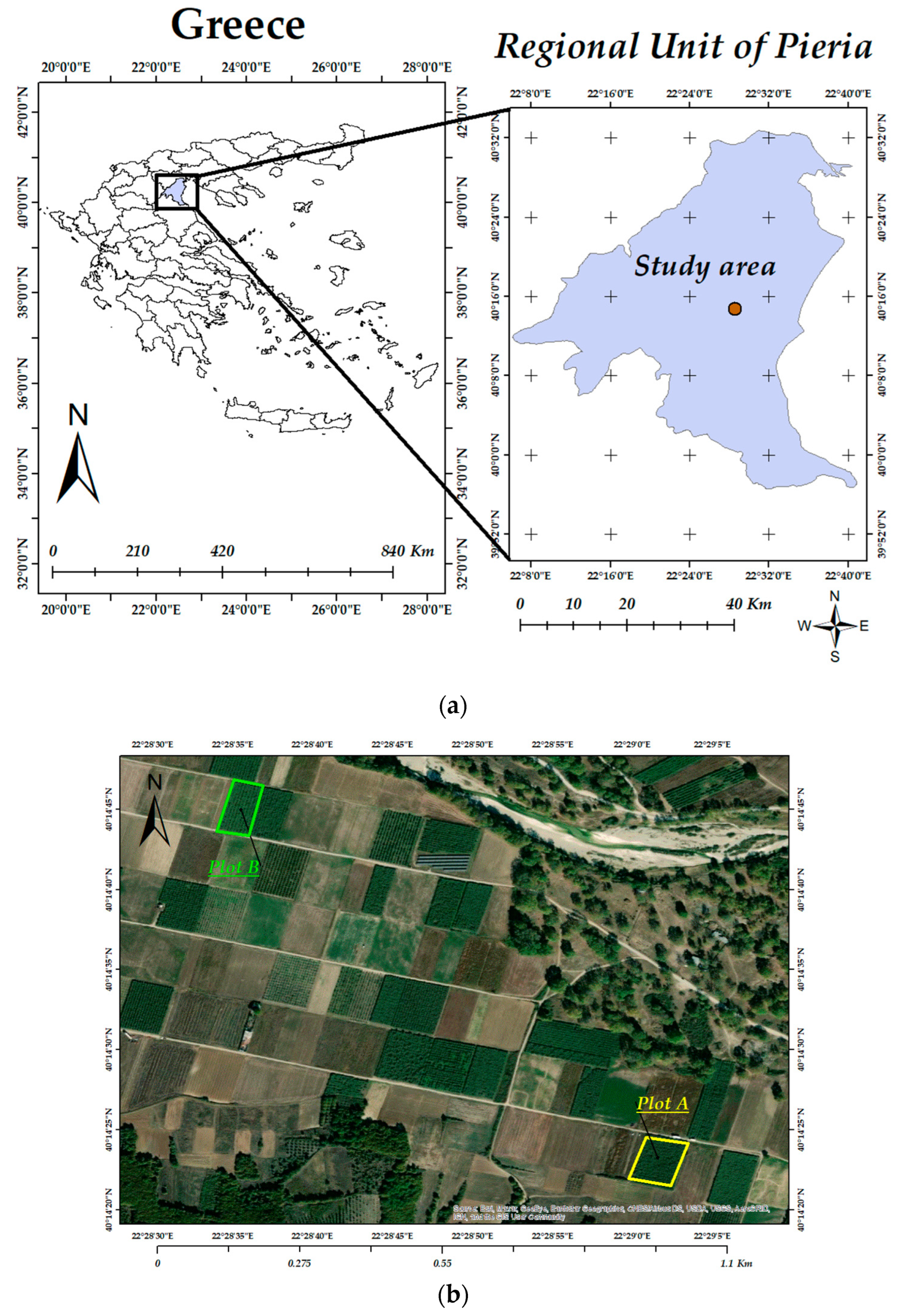
2.1. Study Site Description

The study area was located in the regional unit of Pieria, region of Central Macedonia, northern Greece (Figure 1a). Kiwi (Actinidia deliciosa) production was monitored in two nearby, smallhold, grower-managed orchards: plots A and B (Figure 1b), for two consecutive growing seasons (2020 and 2021). Plot A (40°14′22.43″ N, 22°29′1.53″ E), with elevation of 32 m above sea level (a.s.l.), covered an area of 0.50 ha. Plot B (40°14′44.73″ N, 22°28′35.39″ E), with elevation of 32 m a.s.l., was 0.65 ha. The grower in plot B was offered advice about irrigation, fertilization, and pesticides from the gaiasense system, based on site-specific climatic, soil, and plant nutrition data [39].
The climate of the area is typical Mediterranean [40]. Monthly meteorological data of the study area during 2020 and 2021 are shown in Table 1. The soils in both plots are classified as Fluvisols [41]. Soil quality properties of the two plots are summarized in Table 2. Soil textural classification was the same for both plots throughout the soil profile and the majority of the determined chemical properties were also at similar levels. Kiwi trees in both plots were 10 years of age at the beginning of the study. The kiwi cultivar was Tsechelidis in plot B and cv. Hayward in plot A. The vines of cv. Tsechelidis were planted at a spacing of 2 × 5 m, whereas the vines of cv. Hayward at 3 × 3 m. The vines in both sites were trained in a pergola trellis system. Crop harvest was conducted from 25–27 October 2020 and 31 October–1 November 2021 in plot A, whilst in plot B it was on 9 September 2020 and 14 September 2021.

2.2. Irrigation Management

The irrigation system used in both plots was drip irrigation. The same water source was used for the irrigation of both plots. Irrigation water quality characteristics are presented in Table 3. The total amount of irrigation water applied to plot A during the 2020 growing season was 756 mm. During the 2021 growing season, however, it increased to 1350 mm. The total amount of irrigation water applied to plot B was 599 mm and 828.90 mm for the 2020 and 2021 growing seasons, respectively. The higher amounts of irrigation applied to both plots in 2021, compared to 2020, were associated with the lower precipitation during the crop growing season in 2021 (Table 2). The total amount of irrigation water applied to plot B was lower, compared to plot A, in both years of the study. Table A1 presents in detail the irrigation management calendar for both plots.

2.3. Nitrogen Fertilization Management

Nitrogen fertilizer application to kiwi crops was predominantly carried out through broadcasting and fertigation in both plots. Low amounts of N fertilizer were also added through foliar application. The same fertilizers were used in both plots, however, the amounts and dates of application were different. The total amount of N fertilizer applied to plot A was 231.1 kg N ha−1 and 197.2 kg N ha−1 in 2020 and 2021, respectively. The total amount of N fertilizer applied to plot B was 150.1 kg N ha−1 and 176.3 kg N ha−1 in 2020 and 2021, respectively. Plot B received lower N fertilization, compared to plot A, in both years of study. Analytical information about the N fertilization management practices in both plots is summarized in Table 4.

2.4. Field Measurements and Analysis

Each year, in each plot, soil samples were collected in triplicate, three times in the crop growing season; namely on 12 May 2020 (samples taken from both plots), 16 July 2020 (both plots), 23 September 2020 (plot B), 31 October 2020 (plot A), 26 February 2021 (both plots), 16 July 2021 (both plots), 10 September 2021 (plot B), and 01 November 2021 (plot A). The reason why the third sample was collected on different dates for each plot is associated with the different harvest dates in each plot as already mentioned in Section 2.1. Soil samples were collected with a soil sampler at three soil depths (0–30 cm, 30–60 cm, 60–90 cm), placed in polyethylene bags, and transferred to the laboratory for soil analysis. The received soil samples were air-dried at room temperature (20–25 °C), gently crushed, and passed through a 2 mm sieve to be used for analysis. Soil samples were analyzed for nitrate (NO3) and ammonium (NH4) nitrogen. Both NO3 and NH4 ions available in soil were extracted with 2 M KCl and they were measured using UV–Vis spectrometry and the sodium salicylate–sodium nitroprusside method, respectively [42,43]. Annual yield data were provided by the grower of each plot.

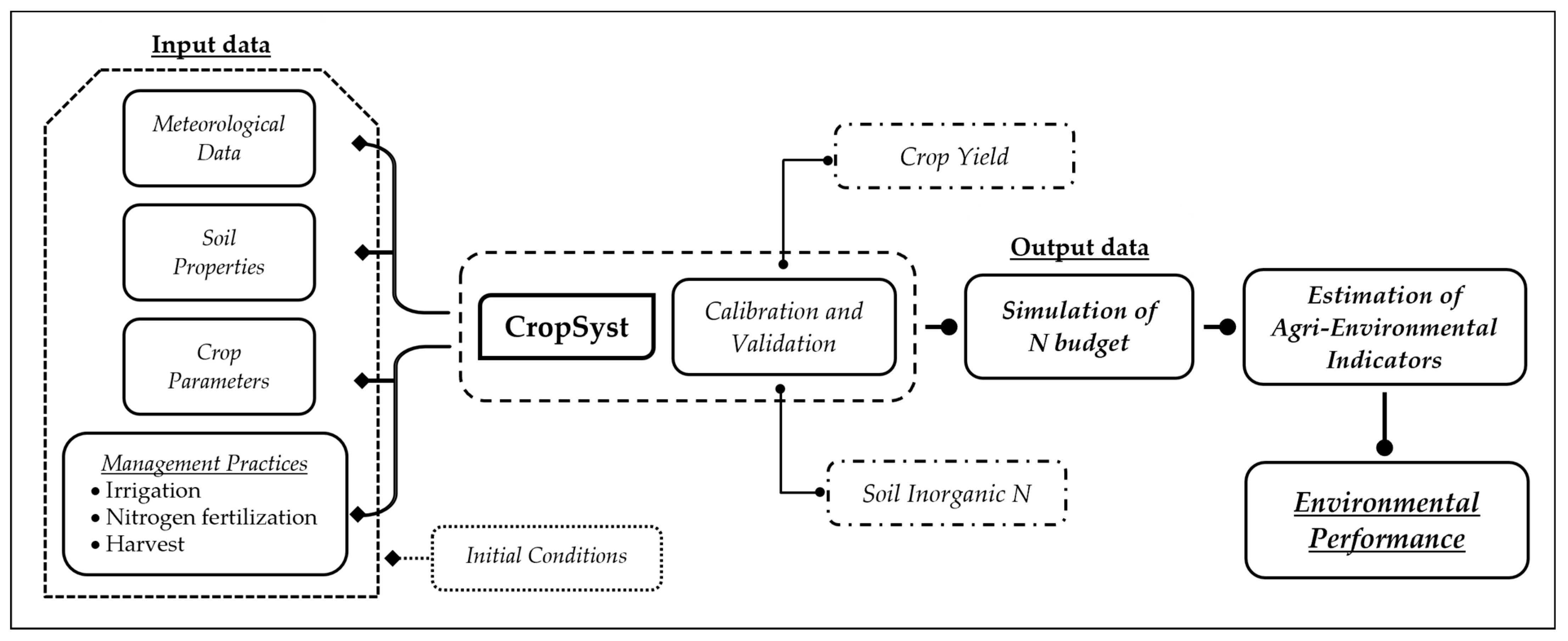
2.5. Model Description and Calibration

2.5.1. Model Description

Crop growth simulation model CropSyst was used to simulate kiwi yield and N budget. CropSyst simulates the soil–water budget, soil–plant N budget, crop phenology, canopy and root growth, biomass production, crop yield, residue production and decomposition, soil erosion by water, and salinity [36]. These processes are affected by weather, soil characteristics, crop characteristics, and cropping system management options including, among others, irrigation and N fertilization. The model has been evaluated in many locations around the world by comparing model estimates to data collected in field experiments [36].
The mineral N budget in the CropSyst model includes separate budgets for nitrate and ammonium and the processes used are N transport, N transformations, ammonium sorption, crop N uptake, and residue mineralization. The method developed for CropSyst for N transport through the soil profile is similar to that described by Corwin et al. [44]. The N transformations developed for CropSyst include net mineralization, nitrification, and denitrification, which follow the approach presented by Stöckle and Campbell [45] using first order kinetics and are assumed to occur in the top 30 to 50 cm of the soil profile. Crop N uptake was modeled by modifying the approach of Godwin and Jones [46] where N uptake is determined as the minimum of crop N demand and potential N uptake. Crop N demand is the amount of N the crop needs to meet its potential growth, as limited by light, temperature, and water, plus its deficiency demand. Yield simulation depends on total biomass accumulated at physiological maturity (BPM) and the harvest index (HI = harvestable yield/aboveground biomass) [36]. The harvest index is determined using as a base an unstressed harvest index modified according to stress intensity (water and N) and crop sensitivity to stress during flowering and grain filling.

2.5.2. CropSyst Calibration, Validation, and Evaluation

Although the model leads to improved decision making in fertilization and water management, it needs to be calibrated and validated through specific field experiments to be used in certain areas. In our study, two-year field data were used for model parameterization. CropSyst was calibrated for one year and then validated for the other year, separately for each plot. The parameters calibrated by the model include crop as well as soil parameters. During calibration, the difference between the simulation and observation result was minimized by a trial-and-error approach. After calibration, the model was validated by applying the calibrated set of parameters to the other year for plot A and plot B.
The evaluation of the CropSyst model was performed by comparing the observed and simulated values of yield and soil inorganic N (0–90 cm depths) over the growing season. Specifically, the model’s simulation performance was evaluated using the statistical criteria (Equations (1)–(5)) of the mean absolute error (ΜAE), the mean absolute percentage error (MAPE), the percent bias (PBIAS), the root mean square error (RMSE), and the normalized root mean square error (NRMSE). Mean absolute error (ΜAE) indicates the average magnitude of the errors in observed and simulated values, without considering their direction, while mean absolute percentage error (ΜAPE) measures the size of the error in percentage terms. The percent bias (PBIAS) measures the average tendency of the simulated values to be larger or smaller than their observed ones. The optimal value is zero, with low-magnitude values indicating accurate model simulation. Positive values of PBIAS indicate overestimation bias whereas negative values indicate model underestimation bias. The root mean square error (RMSE) expresses the variance of errors and ranges from zero to positive infinity, with the model’s performance improving as it approaches zero. The normalized root mean square error (NRMSE) can be interpreted as a fraction of the overall range that is typically resolved by the model with values between zero and one.
M A E = i = 1 n | O i S i | n
M A P E = i = 1 n | O i S i | O i n × 100
P B I A S = i = 1 n ( S i O i ) i = 1 n O i × 100
R M S E = i = 1 n ( O i S i ) 2 n
N R M S E = R M S E O ¯
where: n is the number of observations, O is the mean of the observations, Si and Oi are the simulated and observed values, respectively.

2.6. Environmental Performance Indicators

To assess the environmental consequences of the different irrigation and N fertilization management practices in kiwi production, the following agri-environmental indicators were evaluated for the two plots. Agri-environmental indicators provide information on environmental as well as agronomic performance [47,48].

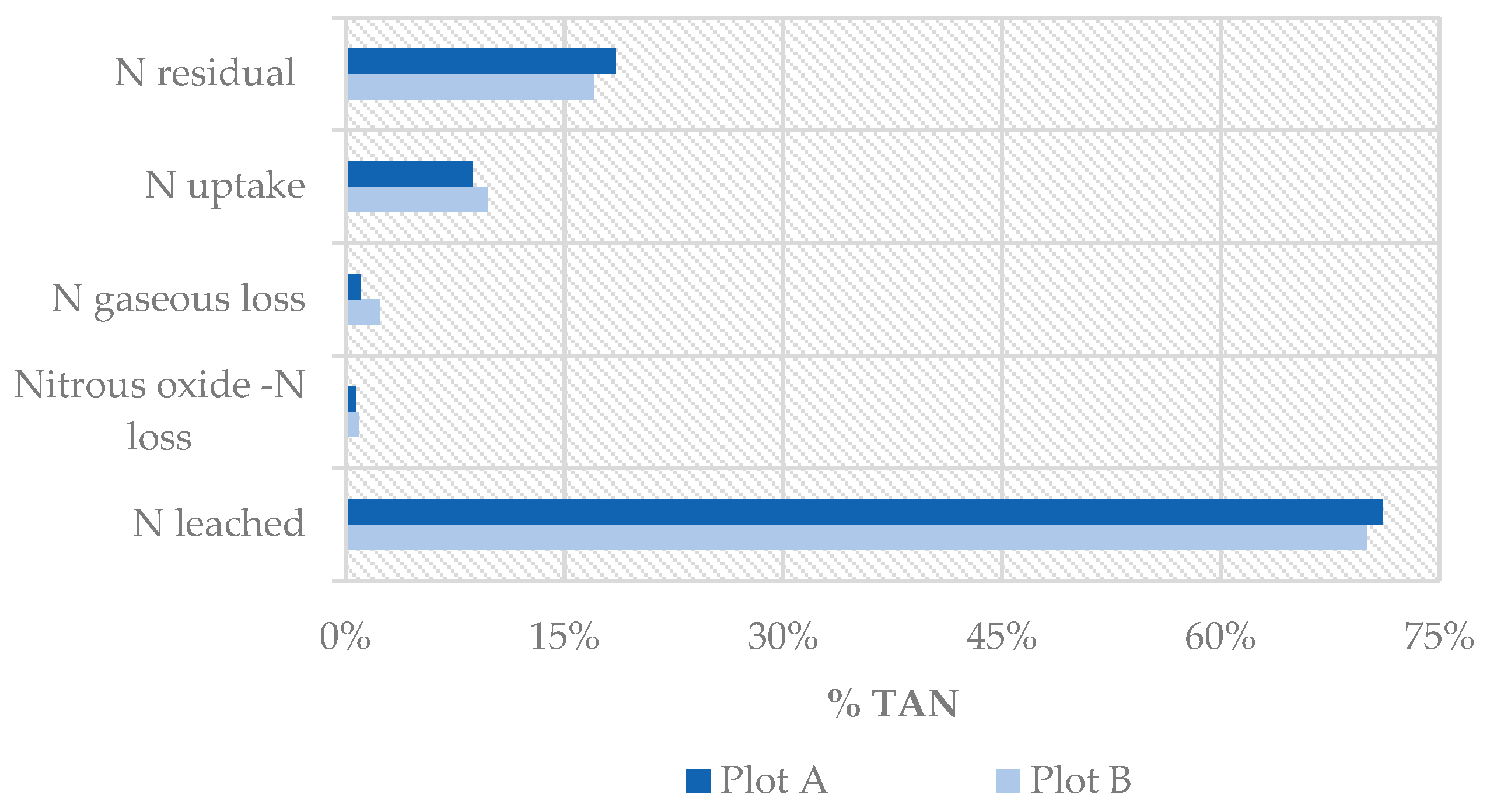
2.6.1. Nitrogen Budget Components (%TAN)

Nitrogen budget components as a percentage of total available soil nitrogen (% TAN) express the outputs of N budget, namely N uptake, N leached, and N lost in the atmosphere, and also the residual soil N, as a percentage of the total available nitrogen (TAN) in the soil profile. Total available nitrogen (TAN) (kg N ha−1) was calculated as the sum of total inorganic N applied as fertilizer (FN), the initial inorganic N in the soil profile (0–90 cm) (SN), and the net mineralized N (Nmin) (Equation (6)).
TAN = FN + SN + net Nmin
The net mineralized N was estimated as the difference between the mineralized N and the immobilized N during the crop growing season and was simulated by the CropSyst model. N uptake (kg N ha−1) was simulated by the CropSyst model and refers to crop N removal. N environmental losses by leaching (leached N), nitrification, denitrification, and volatilization (N2O losses and N gaseous losses) during the crop growing season were also simulated by the CropSyst model in kg N ha−1.

2.6.2. Residual Soil Nitrogen (kg N ha−1)

Residual soil nitrogen (RSN) shows the amount of inorganic N (ammonium and nitrate) that remains in the soil at the end of the growing season after crops have been harvested, for the 0–90 cm depths.

2.6.3. Nitrogen Productivity Factor (kg N Mg−1)

Nitrogen productivity factor (NPF) was calculated as the amount of N fertilizer applied per unit of yield (Equation (7)).
N P F = F N Y s
where: Ys is the simulated yield of kiwi crop (Mg ha−1) and FN is the amount of N fertilizer applied (kg N ha−1).

2.6.4. Irrigation Water Productivity (m3 Mg−1)

Irrigation water productivity (IWP) was determined as the simulated yield obtained per unit of irrigation water applied (kg m−3) (Equation (8)) and is an index of water use efficiency by the crop. This indicator considers just the total amount of water applied by irrigation, or irrigation water use (IWU), with no distinction of what part is consumed as ETc, LF, or N-BWU. ETc is the crop evapotranspiration and LF is the leaching fraction, which must be considered when there is a risk of salt accumulation in the root zone. N-BWU is the non-beneficial water use, i.e., the water that is lost through percolation, runoff out of the cropping site, and wind drift when sprinkling irrigation is applied.
I W P = Y s I W U
where: Ys is the simulated crop yield (103 kg ha−1) and IWU is the total amount of the applied irrigation water (m3 ha−1). This equation, however, has the limitation of not considering the effect of precipitation on crop performance.

2.6.5. Estimation of Environmental Performance

The environmental performance of kiwi production was evaluated, based on the above agri-environmental indicators estimated for the two kiwi orchards under study, taking into consideration the different irrigation and N fertilization management practices applied to each orchard. Figure 2 shows a flowchart that summarizes the approach for the environmental performance evaluation. As presented in Figure 2, the input data for the elaboration of the CropSyst model included meteorological data, soil properties, crop parameters, management practices, and the required initial conditions. Following model calibration and validation for crop yield and soil inorganic N for 2020 and 2021 growing seasons, N budget was simulated (including soil inorganic N, N uptake, leached N, and N lost to the atmosphere). Based on N budget simulation results, agri-environmental indicators were estimated and the environmental effects of the different irrigation and N fertilization management practices applied to kiwi orchards were evaluated.

3. Results and Discussion

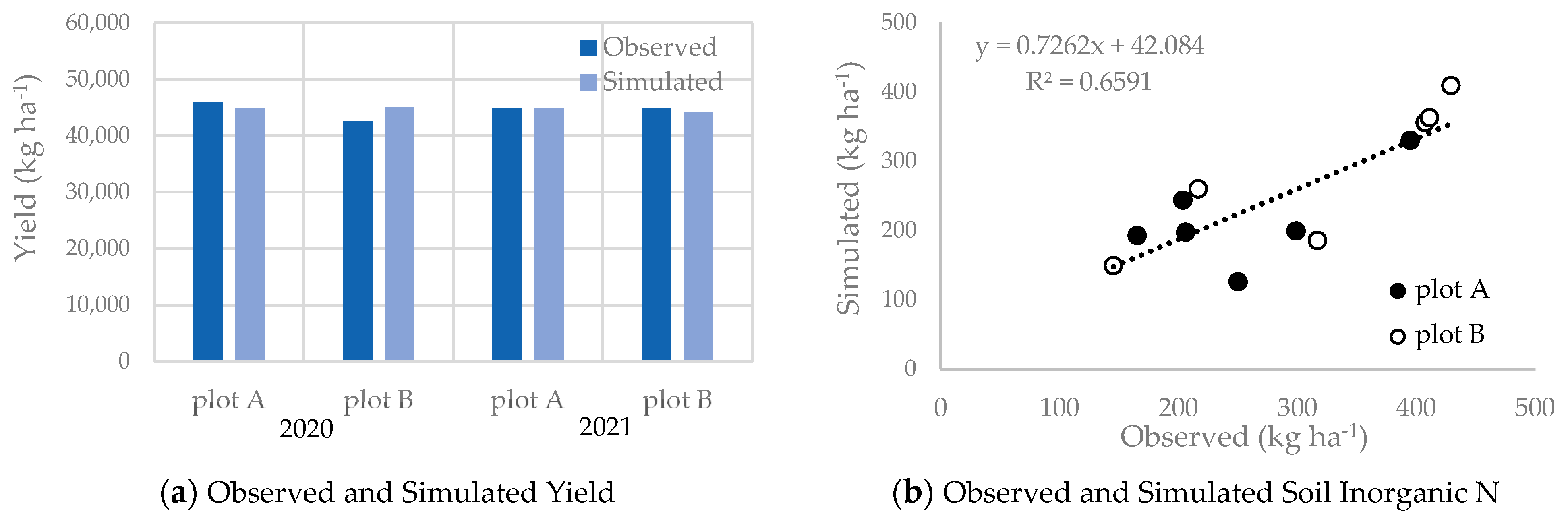
3.1. Model Performance

The observed and simulated yields by the CropSyst model for the two plots for the years 2020 and 2021 are shown in Figure 3a while in Figure 3b the comparison of observed and simulated soil inorganic N within the 0–90 cm depths in 2020 and 2021 is presented. The statistical criteria for the model evaluation in simulating yield and inorganic N are shown in Table 5.
The comparison between the observed and simulated yields illustrated a good agreement between measured and predicted values by the CropSyst model, as a low percentage of difference between observed and simulated values existed (Table 5). The mean absolute percentage error (MAPE) was low, showing the model’s highly accurate prediction, with the mean absolute error (MAE) being 108 kg ha−1. The value of percent bias (PBIAS) is close to zero, indicating very good performance of the model in yield simulation. The root mean square error (RMSE) was 1422.96 kg ha−1 and normalized root mean square error (NRMSE) was close to zero, showing the very good performance of the model.
The simulation of soil inorganic N (0–90 cm depths) compared relatively well with the measured data. R2 (Pearson’s correlation coefficient) describes the proportion of the variance in observed data explained by the model with values greater than 0.5 being considered acceptable (R2 = 0.6591). Mean absolute percentage error was 19.44%, indicating a good prediction by the model. The model had a mean absolute error of 55.45 kg N ha−1. This value, although it is not negligible, constitutes only 5.2% of the mean TAN and therefore was considered acceptable. RMSE value was 68.87 kg N ha−1 and NRMSE was 0.24, showing a relatively good performance by the CropSyst model. PBIAS had a negative low value indicating the model’s good performance and underestimation of soil inorganic N.

3.2. Simulation of N Budget

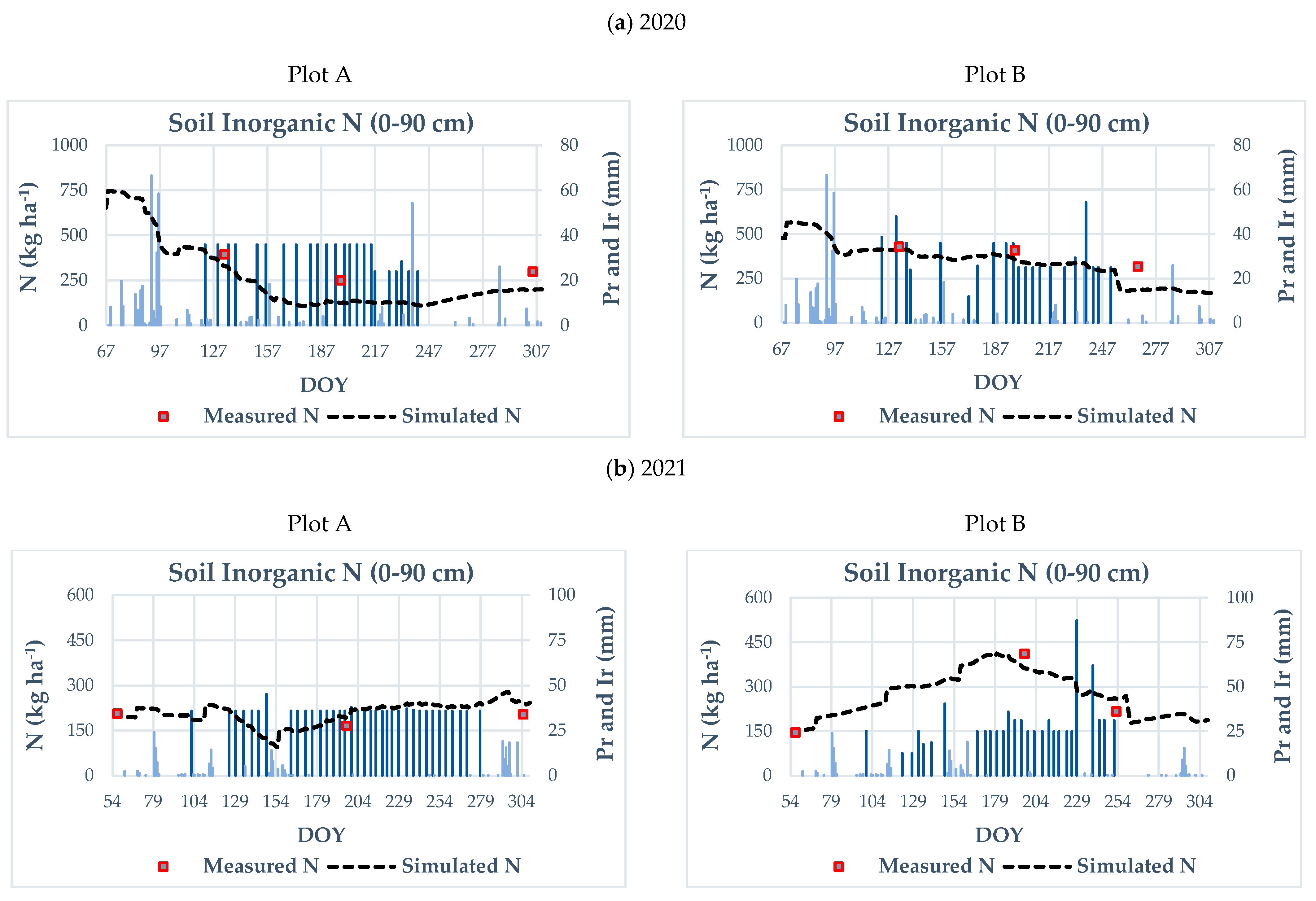
3.2.1. Soil Inorganic N

Simulated inorganic N (sum of NH4-N and NO3-N) fluctuation within the soil profile (0–90 cm depths) on a daily basis for both plots and years of study is presented in Figure 4. The pattern of inorganic N fluctuation differed between the plots and the years mainly due to the different irrigation and fertilization management practices and weather conditions (from year to year). Inorganic N content was high at the beginning of the 2020 growing season in both plots (655 kg N ha−1 and 477 kg N ha−1 in the top 90 cm in plots A and B, respectively). Other studies in medium-textured soils in the Mediterranean region have also found similarly high values. Villar-Mill et al. [49] reported a range of 123 to 459 kg NO3-N ha−1 in the top 120 cm, Vazquez et al. [50] reported 851 kg inorganic N ha−1 in the top 100 cm, and Vazquez et al. [51] reported 453 kg inorganic N ha−1 in the top 100 cm. During the growing season, soil inorganic N presented a decreasing trend; the residual soil inorganic N was up to 70% lower in relation to the initial N, suggesting potential N leaching losses. In the 2021 cultivation period, the initial soil inorganic N was at lower levels compared with 2020 (206 kg N ha−1 and 145 kg N ha−1 in the top 90 cm in plots A and B, respectively).

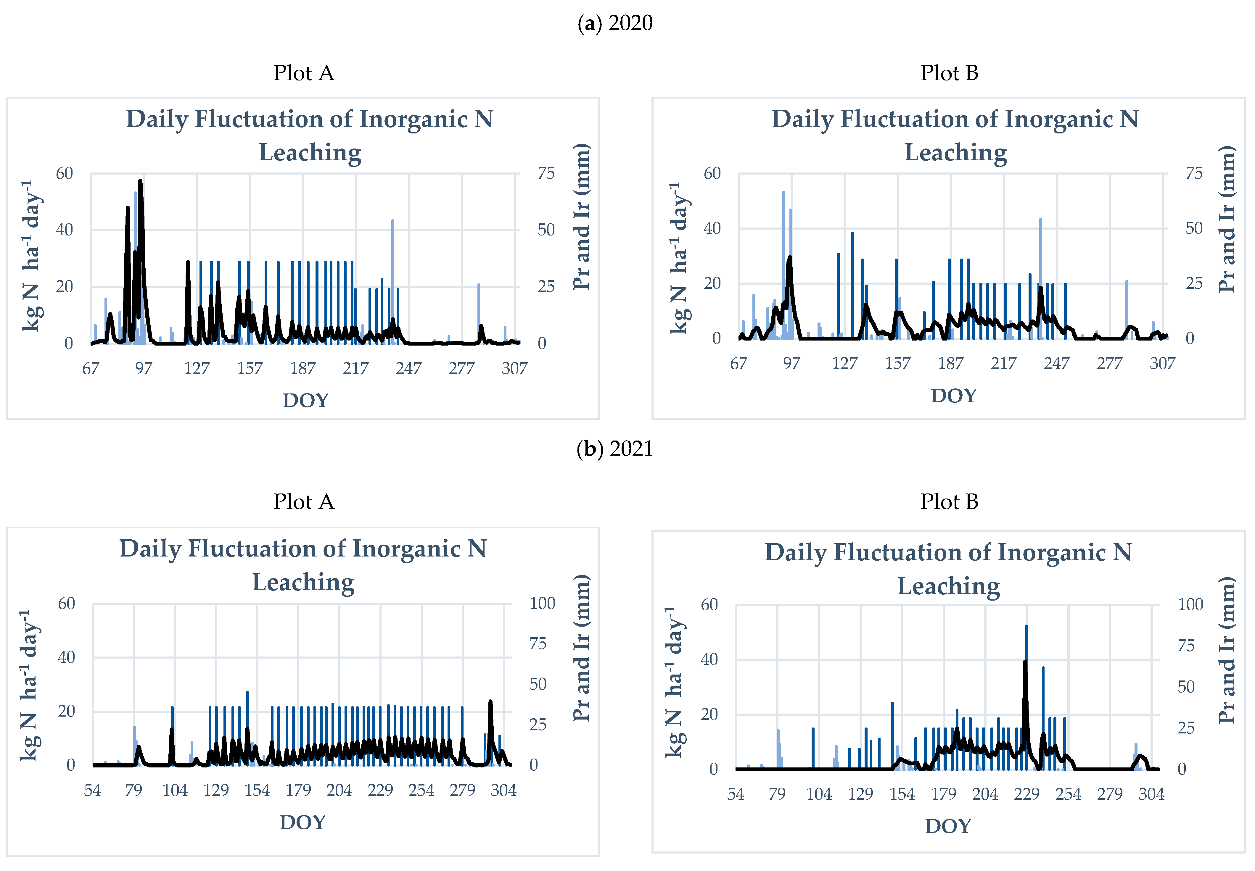
3.2.2. N Leaching Losses

The inorganic N leached (sum of NH4-N and NO3-N) below the 90 cm depths on a daily basis, as simulated by CropSyst model, for plots A and B in both years of study is shown in Figure 5. In 2020, for both plots under study, high daily N leaching rates (maximum up to 57.5 kg N ha−1 day−1 and 29.6 kg N ha−1 day−1 for plots A and B, respectively) occurred early in the growing season, following the application of the first dose of N fertilizer and about a 2-week period of rainfall (including three rainfall events of 66.6, 32.4, and 58.5 mm day−1 towards the end of this 2-week period). Despite the high soil inorganic N content in the profile at the beginning of the growing season, the growers of both plots applied the basic N fertilizer dose (96 kg N ha−1, Table 4) according to the standard practices in the area. This management practice, in conjunction with the weather conditions, most probably resulted in the high N leaching rates. Towards the end of the growing season, daily N leaching rates were very low. Other studies have already shown the dependency of N leaching on both the total amount of precipitation and its distribution throughout the year [10,13]. The daily N leaching pattern in 2021 was very different compared to 2020, mostly due to the different weather conditions, irrigation, and N fertilizer application. In 2021, the daily N leaching pattern also differed between the two plots. This could be mainly attributed to the different N fertilizer and irrigation management practices. Maximum daily N leaching rate was 23.8 kg N ha−1 day−1 and 39.4 kg N ha−1 day−1 for plots A and B, respectively.

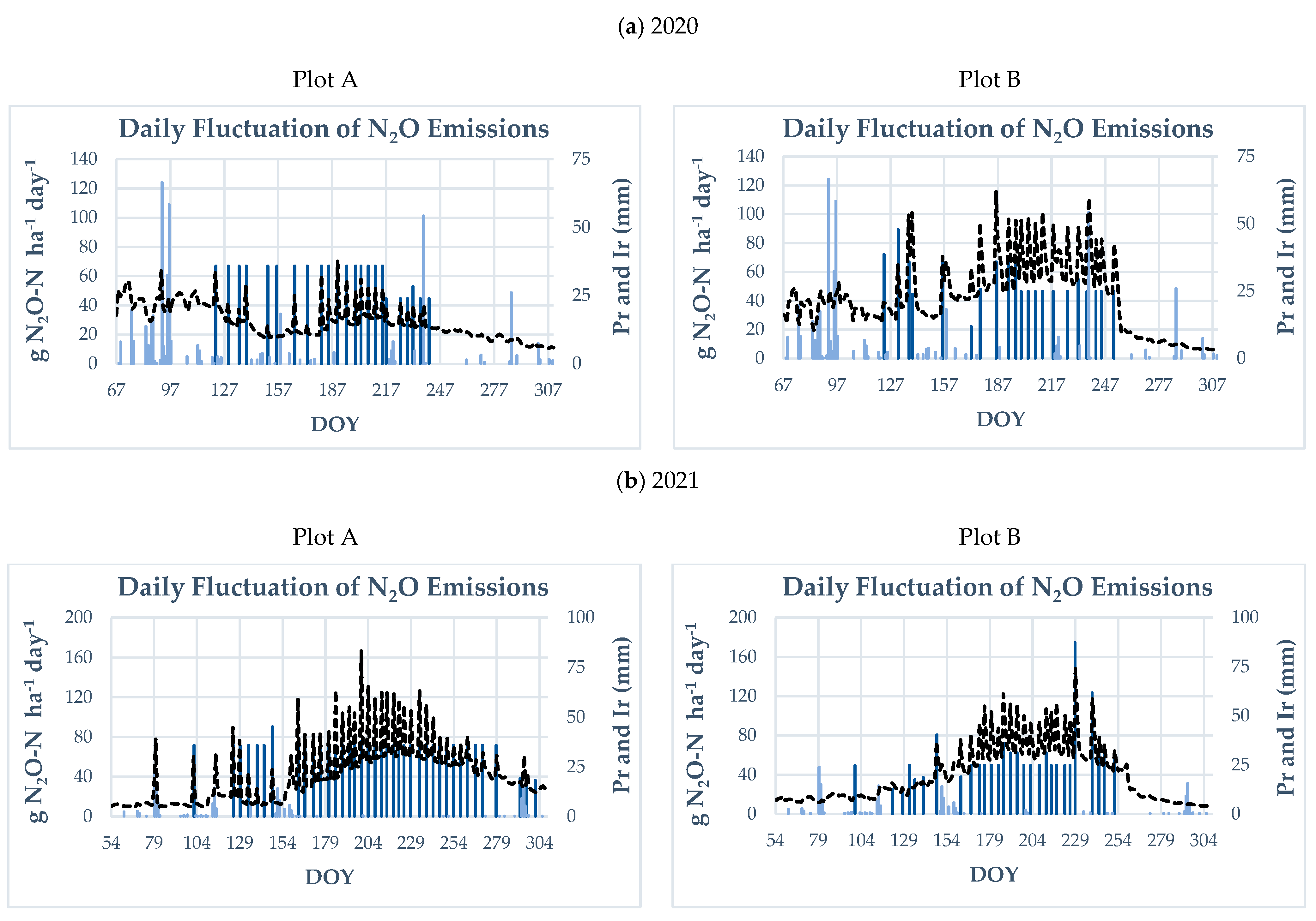
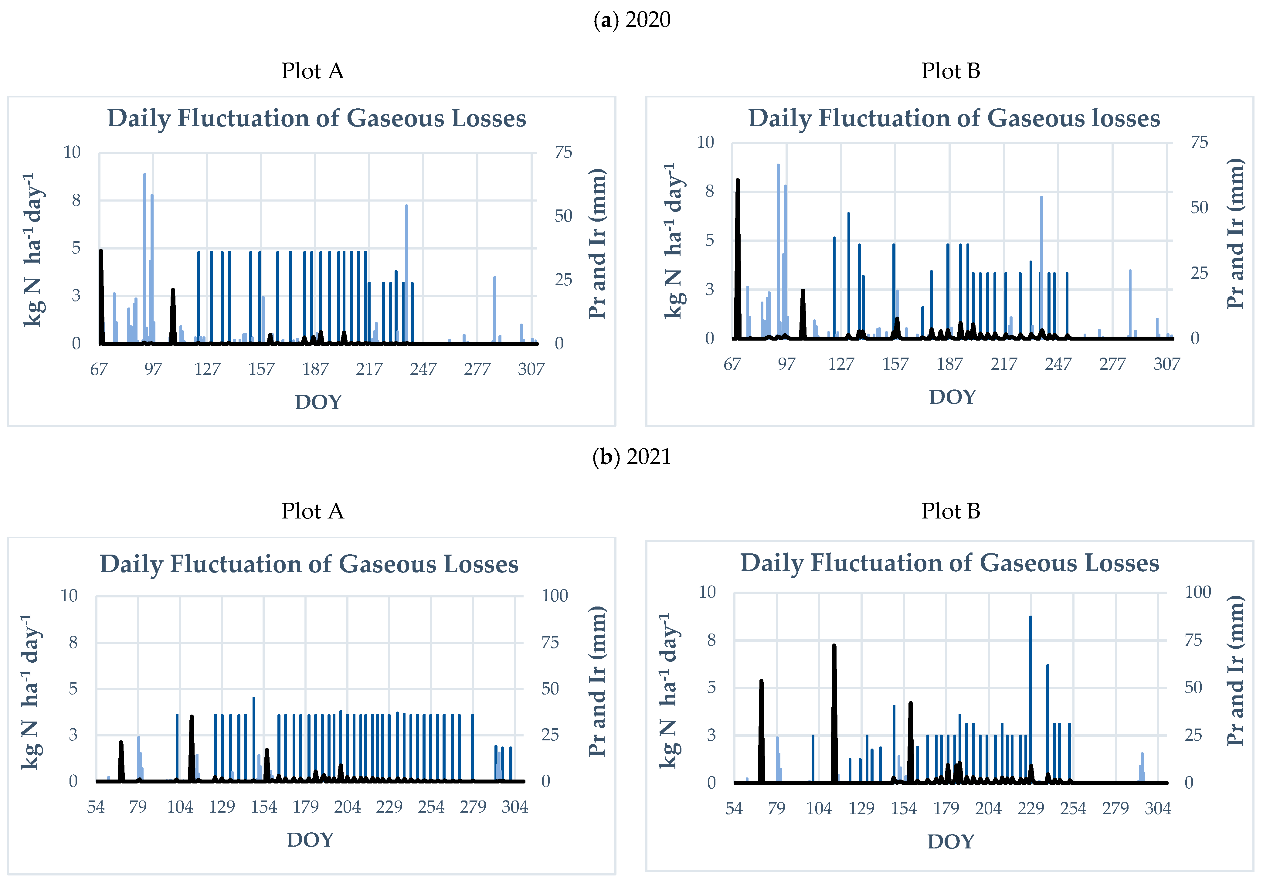
3.2.3. Atmospheric N Losses

A large number of peaks of simulated daily nitrous oxide (N2O) emissions were detected during 2020 and 2021 concerning both plots (Figure 6). The large number of peaks are a result of the combination of many fertilizer applications and irrigation events during the cultivation periods (Table 4 and Table A1). During 2020, the largest N2O peak, being observed about four months after the first application, was 70 g N2O-N ha−1 day−1 regarding plot A and 110 g N2O-N ha−1 day−1 in the case of plot B. In 2021, daily emissions were larger compared to 2020, reaching about 170 g N2O-N ha−1 day−1 and 150 g N2O-N ha−1 day−1 in plots A and B, respectively. The increase in daily N2O emissions in 2021 may be predominantly associated with the increased amount of irrigation water applied, compared to 2020.
In both plots and years of study, N gaseous losses were predominantly associated with N fertilizer application with the method of broadcasting. As shown in Figure 7, regarding plot A, the largest peak of gaseous N losses was 4.86 kg N ha−1 day−1 in 2020 and 3.51 kg N ha−1 day−1 in 2021. In the case of plot B, the largest peak of gaseous N losses was 8.08 kg N ha−1 day−1 in 2020 and 7.24 kg N ha−1 day−1 in 2021. All peaks, in both plots, corresponded to the highest amount of N fertilizer applied by broadcasting early in the growing season (see Table 4).

3.2.4. Kiwi N Uptake

Simulated kiwi N uptake was comparable for both plots in both years of study. Mean N uptake was 103.3 kg ha−1 (it ranged between 102.8 and 103.7 kg N ha−1 between the different plots and years of study).

3.3. Environmental Performance: Agri-Environmental Indicators

Agri-environmental indicators were calculated based on the N budget simulation results to assess the environmental consequences (focusing on N losses) of the different irrigation and N fertilization management practices in kiwi production. Figure 8 illustrates the arithmetic mean of the outputs of N budget, namely N uptake, leached N, and N lost in the atmosphere (N2O and gaseous loss), and also the residual soil N, as percentage of the total available nitrogen (TAN) in the soil profile, based on CropSyst simulation results, for the 2020 and 2021 growing seasons. N leaching losses were higher in plot A in relation to plot B, indicating higher environmental threat to groundwater quality during the cultivation periods. A slightly higher percentage of residual N was observed in the case of plot A, while N uptake and N atmospheric losses were lower compared to plot B. The emission factor (EF) for direct N2O losses from both plots was within the IPCC EF1 uncertainty range of 0.3–3% [52]. N losses (sum of atmospheric and N leaching losses) were up to 73.3% of TAN. Other research has illustrated that N losses to the environment accounted for 77.2% of total N input in kiwi orchards in China [53] and 76% of N fertilizer inputs in olive groves in Portugal [54]. In absolute values, N losses were 866.8 kg N ha−1 and 786.1 kg N ha−1 for plots A and B, respectively; hence, an increase of about 10% in N losses was found for plot A compared to plot B. The management practices in plot B involved lower application of both irrigation water and N fertilizer (by 32.2% and 23.8%, respectively, considering the total amount applied in both years in plot A). Consequently, the reduced irrigation and N fertilization resulted in lower N losses, whilst crop yield and N uptake were similar for both plots.
Mean N leaching losses were 845.86 and 752.28 kg N ha−1, for plots A and B, respectively. Other research work in drip-irrigated crops in the Mediterranean region has shown nitrate N leaching losses ranging from 431 to 891 kg NO3-N ha−1 [50]. Mean N leaching losses expressed as a percentage of TAN (Figure 8) were higher than 70% in both plots. This high percentage of TAN leached below the 90 cm depths during the crop growing season, hence influencing groundwater quality. Kiwifruit vines have a relatively shallow rooting system, with the critical root zone distributed within the top 60 cm depths [55]. Consequently, more than 70% of TAN, which leached below the root zone, could not be used by kiwi and contributed to groundwater pollution. Therefore, kiwi production posed a severe threat to the environment in both orchards under study and management practices need to be improved. Gao et al. [56], in their study, showed that more than 77.5% of nitrate leached below the root zone in kiwi orchards in China. Optimizing water and fertilizer management practices appears to be the primary approach for reducing N leaching [57].
Mean residual soil N was lower in plot B compared to plot A (Table 6), thus indicating the lower potential risk for N leaching following the growing season in plot B in relation to plot A. The lower residual N in plot B may be attributed to the lower N fertilizer applied. Other research has also shown that nitrate N accumulation in soil increased with increasing N application rates [10,57,58].
NPF was lower in plot B compared to plot A (Table 6) because of the lower N fertilizer addition per Mg of product, suggesting the better N use efficiency in plot B. According to Koukoulakis and Papadopoulos [59], N removal by kiwifruit harvest is 120 kg N ha−1 for a yield of 30 Mg ha−1, suggesting an average N removal rate by the crop of 4 kg N Mg−1 of product. This value is in good agreement with the calculated NPF, especially in the case of plot B.
The amounts of N fertilizer applied by the growers in the two plots under study ranged from about 150 to 230 kg N ha−1. These amounts of N fertilizer may fully cover or be in excess of crop requirements, as kiwifruit require approximately 150 kg Ν ha−1 year−1 [8]. Soil inorganic N constitutes a source of available N for plant uptake and should be taken into consideration to optimize N fertilization. As already shown in Figure 4, the soil inorganic N content in the profile was not negligible in both plots and years of study, suggesting that the amount of N fertilizer applied was higher than necessary. Over-fertilization with N results in N surplus causing large amounts of residual inorganic N in soil [13,58] which can be easily leached into deep soil layers, resulting in negative environmental impacts [14,60].
Finally, IWP was higher in plot B compared to plot A (Table 6), suggesting higher kiwifruit production per m3 of irrigation water applied, hence demonstrating the better water use efficiency by kiwi in plot B. Both plots, however, were over-irrigated. Irrigation water needs (IrN) of kiwi crops were estimated (not simulated) on a monthly basis as the difference between crop evapotranspiration (ETc), calculated according to Allen et al. [61], and effective precipitation (Pe), determined according to the USDA [62] (Table 7). As shown in Table 7, in most cases, the amount of irrigation water applied to both plots was higher than crop irrigation water needs; higher than double the needs in certain months. The excessive amount of irrigation water applied, apart from causing waste of resources, potentially increased drainage and consequently N leaching. Other studies have shown increased nitrate leaching with increased irrigation [59,60,63].
The above results clearly present that kiwifruit was over-irrigated and over-fertilized with N in the area. The over-irrigation and over-fertilization with N occurred in both orchards under study and may explain the high percentage of TAN leached below the 90 cm depths during the crop growing season.

4. Conclusions

The CropSyst model was calibrated and validated with field measurements in two kiwi orchards in northern Greece during two consecutive growing seasons. According to CropSyst model simulation results, the simultaneous reduction in N fertilizer and irrigation water inputs to kiwi production resulted in similar yields and N uptake, but lower N leaching losses during the crop growing season. Additionally, it resulted in lower RSN and hence lower potential risk for N leaching following the cultivation period and lower NPF and IWP, indicating better N and water use efficiency. More than 70% of total available N leached below the 90 cm depths during the crop growing season in both study sites, due to over-irrigation and over-fertilization with N, posing a potential threat to groundwater quality.
This study has pointed out the necessity for improved irrigation and N fertilizer management for sustainable kiwi production in the area. Further work is necessary to determine the optimal N fertilizer and irrigation water management strategies.

Author Contributions

Conceptualization, M.K., P.K., D.K. and P.G.; methodology, M.K., P.K., D.K. and P.G.; software, M.K. and P.K.; validation, M.K., P.K., D.K. and P.G.; data curation, M.K., P.K., D.K. and P.G.; writing—original draft preparation, M.K. and P.K.; writing—review and editing, M.K., P.K., D.K. and P.G.; supervision, D.K. and P.G.; project administration, M.K., P.K., D.K. and P.G.; funding acquisition, M.K., P.K., D.K. and P.G. All authors have read and agreed to the published version of the manuscript.

Funding

This research was part of the project with contract number LIFE17 ENV/GR000220 entitled “LIFE GAIA Sense: Innovative Smart Farming services supporting Circular Economy in Agriculture” which is co-funded by the LIFE Programme of the European Union.

Data Availability Statement

The datasets generated and analyzed during the current study are available from the corresponding author on reasonable request.

Conflicts of Interest

The authors declare no conflict of interest.

Appendix A

Table A1. Irrigation management calendars for plots A and B in 2020 and 2021.
Irrigation Management Practices 2020Irrigation Management Practices 2021
Plot A Plot B Plot A Plot B
Date of ApplicationIrrigation (mm)Date of ApplicationIrrigation (mm)Date of ApplicationIrrigation (mm)Date of ApplicationIrrigation (mm)
1 May362 May3611 April369 April25
8 May3610 May484 May361 May12.5
14 May3616 May368 May367 May12.5
18 May3618 May2413 May3611 May25
30 May364 June3618 May3614 May12.5
4 June3620 June1222 May3619 May18.75
14 June3625 June2427 May3627 May31.2
21 June364 July3611 June3610 June18.75
29 June3611 July3615 June3616 June25
3 July3615 July3620 June3621 June25
8 July3618 July2524 June3624 June25
13 July3622 July2529 June3628 June25
18 July3626 July253 July362 July25
21 July3630 July257 July365 July36
25 July365 August2511 July369 July31.2
29 July3613 August2514 July3613 July31.2
2 August3619 August2518 July3617 July25
4 August2424 August2522 July3621 July25
12 August2429 August2526 July3626July25
16 August241 September2530 July3630 July31.2
19-August248 September252 August362 August25
23 August24 6 August365 August25
28 August24 9 August3610 August25
12 August3613 August25
16 August3616 August87.5
21 August3626 August62
25 August3630 August31.2
29 August362 September31.2
2 September368 September31.2
6 September36
10 September36
14 September36
18 September36
23 September36
27 September36
5 October36
19 October18
23 October18
28 October18

References

  1. Faostat. 2020. Available online: https://www.fao.org/faostat/en/#home (accessed on 15 July 2022).
  2. Hellenic Statistical Authority. 2019. Available online: https://www.statistics.gr/el/statistics/-/publication/SPG06/- (accessed on 20 August 2022).
  3. Sotiropoulos, T.; Koukourikou-Petridou, M.; Petridis, A.; Stylianidis, D.; Almaliotis, D.; Papadakis, I.; Therios, I.; Molassiotis, A. ‘Tsechelidis’ Kiwifruit. HortScience 2009, 44, 466–468. [Google Scholar] [CrossRef]
  4. Dichio, B.; Montanaro, G.; Sofo, A.; Xiloyannis, C. Stem and whole-plant hydraulics in olive (Olea europaea) and kiwifruit (Actinidia deliciosa). Trees 2013, 27, 183–191. [Google Scholar] [CrossRef]
  5. Holzapfel, E.A.; Merino, R.; Marino, M.A.; Matta, R. Water production functions in kiwi. Irrig. Sci. 2000, 19, 73–79. [Google Scholar] [CrossRef]
  6. Francia, M.; Giovanelli, J.; Golfarelli, M. Multi-sensor profiling for precision soil-moisture monitoring. Comput. Electron. Agric. 2022, 197, 106924. [Google Scholar] [CrossRef]
  7. Torres-Ruiz, J.M.; Perulli, G.D.; Manfrini, L.; Zibordi, M.; Lopéz Velasco, G.; Anconelli, S.; Pierpaoli, E.; Corelli-Grappadelli, L.; Morandi, B. Time of irrigation affects vine water relations and the daily patterns of leaf gas exchanges and vascular flows to kiwifruit (Actinidia deliciosa Chev.). Agric. Water Manag. 2016, 166, 101–110. [Google Scholar] [CrossRef]
  8. Santoni, F.; Barboni, T.; Paolini, J.; Costa, J. Influence of cultivating parameters on the composition of volatile compounds and physicochemical characteristics of kiwi fruit. J. Sci. Food Agric. 2013, 93, 604–610. [Google Scholar] [CrossRef] [PubMed]
  9. Zhang, X.; Davidson, E.A.; Mauzerall, D.L.; Searchinger, T.D.; Dumas, P.; Shen, Y. Managing nitrogen for sustainable development. Nature 2015, 528, 51–59. [Google Scholar] [CrossRef]
  10. Lu, Y.; Kang, T.; Gao, J.; Chen, Z.; Zhou, J. Reducing nitrogen fertilization of intensive kiwifruit orchards decreases nitrate accumulation in soil without compromising crop production. J. Integr. Agric. 2018, 17, 1421–1431. [Google Scholar] [CrossRef]
  11. Lassaletta, L.; Billen, G.; Grizzetti, B.; Anglade, J.; Garnier, J. 50 years trends in nitrogen use efficiency of world cropping systems: The relationship between yield and nitrogen input to cropland. Environ. Res. Lett. 2014, 9, 105011. [Google Scholar] [CrossRef]
  12. Sutton, M.A.; Bleeker, A.; Howard, C.M.; Bekunda, M.; Grizzetti, B.; de Vries, W.; van Grinsven, H.J.M.; Abrol, Y.P.; Adhya, T.K.; Billen, G.; et al. Our Nutrient World: The challenge to produce more food and energy with less pollution. In On behalf of the Global Partnership on Nutrient Management and the International Nitrogen Initiative; Centre for Ecology and Hydrology: Edinburgh, UK, 2013; pp. 1–114. [Google Scholar]
  13. Zhou, J.Y.; Gu, B.J.; Schlesinger, W.H.; Ju, X.T. Significant accumulation of nitrate in Chinese semi-humid croplands. Sci. Rep. 2016, 6, 25088. [Google Scholar] [CrossRef] [PubMed]
  14. Sutton, M.A.; Erisman, J.W.; Leip, A.; Van Grinsven, H.; Winiwarter, W. Too much of a good thing. Nature 2011, 472, 159–161. [Google Scholar] [CrossRef] [PubMed]
  15. Raimondi, G.; Maucieri, C.; Squartini, A.; Stevanato, P.; Tolomio, M.; Toffanin, A.; Borin, M. Soil indicators for comparing medium-term organic and conventional agricultural systems. Eur. J. Agron. 2023, 142, 126669. [Google Scholar] [CrossRef]
  16. de Olde, E.M.; Moller, H.; Marchand, F.; McDowell, R.W.; MacLeod, C.J.; Sautier, M.; Halloy, S.; Barber, A.; Benge, J.; Bockstaller, C.; et al. When experts disagree: The need to rethink indicator selection for assessing sustainability of agriculture. Environ. Dev. Sustain. 2017, 19, 1327–1342. [Google Scholar] [CrossRef]
  17. Westfall, D.G.; Havlin, J.L.; Hergert, G.W.; Raun, W.R. Nitrogen Management in Dryland Cropping Systems. J. Prod. Agric. 1996, 9, 192–199. [Google Scholar] [CrossRef]
  18. Cassman, K.G.; Dobermann, A.; Daniel, T.; Walters, D.T. Agroecosystems, Nitrogen-use Efficiency, and Nitrogen Management. Ambio 2002, 31, 132–140. [Google Scholar] [CrossRef]
  19. Daly, A.B.; Jilling, A.; Bowles, T.M.; Buchkowski, R.W.; Frey, S.D.; Kallenbach, C.M.; Keiluweit, M.; Mooshammer, M.; Schimel, J.P.; Grandy, A.S. A holistic framework integrating plant-microbe-mineral regulation of soil bioavailable nitrogen. Biogeochemistry 2021, 154, 211–229. [Google Scholar] [CrossRef]
  20. Müller, K.; Holmes, A.; Deurer, M.; Clothier, B.E. Eco-efficiency as a sustainability measure for kiwifruit production in New Zealand. J. Clean. Prod. 2015, 106, 333–342. [Google Scholar] [CrossRef]
  21. Salo, T.J.; Palosuo, T.; Kersebaum, K.C.; Nendel, C.; Angulo, C.; Ewert, F.; Bindi, M.; Calanca, A.P.; Klein, T.; Moriondo, M.; et al. Comparing the performance of 11 crop simulation models in predicting yield response to nitrogen fertilization. J. Agric. Sci. 2016, 154, 1218–1240. [Google Scholar] [CrossRef]
  22. Stöckle, C.O.; Martin, S.; Campbell, G.S. CropSyst, a cropping systems model: Water/nitrogen budgets and crop yield. Agric. Syst. 1994, 46, 335–359. [Google Scholar] [CrossRef]
  23. Leghari, S.J.; Hu, K.; Liang, H.; Wei, Y. Modeling water and nitrogen balance of different cropping systems in the North China Plain. Agronomy 2019, 9, 696. [Google Scholar] [CrossRef]
  24. Wajid, A.; Hussain, K.; Ilyas, A.; Habib-ur-Rahman, M.; Shakil, Q.; Hoogenboom, G. Crop models: Important tools in decision support system to manage wheat production under vulnerable environments. Agriculture 2021, 11, 1166. [Google Scholar] [CrossRef]
  25. Janssen, S.; van Ittersum, M.K. Assessing farm innovations and responses to policies: A review of bio-economic farm models. Agric. Syst. 2007, 94, 622–636. [Google Scholar] [CrossRef]
  26. Abi Saab, M.T.; Todorovic, M.; Albrizio, R. Comparing AquaCrop and CropSyst models in simulating barley growth and yield under different water and nitrogen regimes. Does calibration year influence the performance of crop growth models? Agric. Water Manag. 2015, 147, 21–33. [Google Scholar] [CrossRef]
  27. Hammer, G.L.; Kropff, M.J.; Sinclair, T.R.; Porter, J.R. Future contributions of crop modelling from heuristics and supporting decision making to understanding genetic regulation and aiding crop improvement. Eur. J. Agron. 2002, 18, 15–31. [Google Scholar] [CrossRef]
  28. Li, T.; Feng, Y.; Li, X. Predicting crop growth under different cropping and fertilizing management practices. Agric. For. Meteorol. 2009, 149, 985–998. [Google Scholar] [CrossRef]
  29. Todorovic, M.; Albrizio, R.; Zivotic, L.; Abi Saab, M.T.; Stöckle, C.; Steduto, P. Assessment of AquaCrop, CropSyst, and WOFOST models in the simulation of sunflower growth under different water regimes. Agron. J. 2009, 101, 509–521. [Google Scholar] [CrossRef]
  30. Confalonieri, R.; Gusberti, D.; Bocchi, S.; Acutis, M. The CropSyst model to simulate the N balance of rice for alternative management. Agron. Sustain. Dev. 2006, 26, 241–249. [Google Scholar] [CrossRef]
  31. Tahir, N.; Li1, J.; Ma, Y.; Ullah, A.; Zhu, P.; Peng, C.; Hussain, B.; Danish, S. 20 Years nitrogen dynamics study by using APSIM nitrogen model simulation for sustainable management in Jilin China. Sci. Rep. 2021, 11, 17505. [Google Scholar] [CrossRef]
  32. McCown, R.L.; Hammer, G.L.; Hargreaves, J.N.G.; Holzwoth, D.P.; Freebairrn, D.M. APSIM: A novel software system for model development, model testing and simulation in agricultural systems research. Agric. Syst. 1996, 50, 255–271. [Google Scholar] [CrossRef]
  33. Keating, B.A.; Carberry, P.S.; Hammer, G.L.; Probert, M.E.; Robertson, M.J.; Holzworth, D.; Huth, N.I.; Hargreaves, J.N.G.; Meinke, H.; Hochman, Z.; et al. An overview of APSIM, a model designed for farming systems simulation. Eur. J. Agron. 2003, 18, 267–288. [Google Scholar] [CrossRef]
  34. Ebrayi, K.N.; Pathak, H.; Kalhra, N.; Bhatia, A.; Jain, N. Simulation of Nitrogen Dynamics in soil using Infocrop model. Environ. Monit. Assess. 2007, 131, 451–465. [Google Scholar] [CrossRef] [PubMed]
  35. Stöckle, C.O.; Nelson, R.L. CropSyst user’s manual (version 3.0). In Biological Systems Engineering Dept; Washington State University: Pullman, WA, USA, 2000. [Google Scholar]
  36. Stöckle, C.O.; Donatelli, M.; Nelson, R.L. CropSyst: A cropping systems simulation model. Eur. J. Agron. 2003, 18, 289–307. [Google Scholar] [CrossRef]
  37. Sharpley, A.N.; Williams, J.R. EPIC, Erosion, Productivity Impact Calculator: 1 Model Documentation. In U.S. Dept. of Agriculture Technical Bulletin; No. 1768; USA Government Printing Office: Washington, DC, USA, 1990; p. 235. [Google Scholar]
  38. Wagenet, R.J.; Hutson, J.L. LEACM: A Process-Based Model of Water and Solute Movements, Transformations, Plant Uptake and Chemical Reactions in the Unsaturated Zone (Version 2.0); Water Resources Institute, Cornell University: Ithaca, NY, USA, 1989; Volume 2. [Google Scholar]
  39. Fragkou, E.; Tsegas, G.; Karagounis, A.; Barbas, F.; Moussiopoulos, N. Quantifying the impact of a smart farming system application on local-scale air quality of smallhold farms in Greece. Air. Qual. Atmos. Hlth. 2022, 16, 1–14. [Google Scholar] [CrossRef]
  40. Tsanakas, K.; Karymbalis, E.; Gaki-Papanastassiou, K.; Maroukian, H. Geomorphology of the Pieria Mtns, Northern Greece. J. Maps 2019, 15, 499–508. [Google Scholar] [CrossRef]
  41. Aristotle University of Thessaloniki. 2015. Available online: https://iris.gov.gr/SoilServices/ (accessed on 7 April 2023).
  42. Norman, R.J.; Edberg, J.C.; Stucki, J.W. Determination of nitrate in soil extracts by dual-wavelength ultraviolet spectrophotometry. Soil Sci. Soc. Am. J. 1985, 49, 1182–1185. [Google Scholar] [CrossRef]
  43. Nelson, D.W. Determination of ammonium in KCl extracts of soils by the salicylate method. Commun. Soil Sci. Plant Anal. 1983, 14, 1051–1062. [Google Scholar] [CrossRef]
  44. Corwin, D.L.; Waggoner, B.L.; Rhoades, J.D. A functional model of solute transport that accounts for bypass. J. Environ. Qual. 1991, 20, 647–658. [Google Scholar] [CrossRef]
  45. Stöckle, C.O.; Campbell, G. Simulation of crop response to water and nitrogen: An example using spring wheat. Trans. ASAE 1989, 32, 66–74. [Google Scholar] [CrossRef]
  46. Godwin, D.C.; Jones, A.C. Nitrogen dynamics in soil-plant systems. In Modelling Plant and Soil Systems; Hanks, J., Ritchue, J.T., Eds.; American Society of Agronomy: Madison, WI, USA, 1991; Volume 31, pp. 287–321. [Google Scholar]
  47. Langeveld, J.W.A.; Verhagen, A.; Neeteson, J.J.; van Keulen, H.; Conijn, J.G.; Schils, R.L.M.; Oenema, J. Evaluating farm performance using agri-environmental indicators: Recent experiences for nitrogen management in The Netherlands. J. Environ. Manag. 2007, 82, 363–376. [Google Scholar] [CrossRef]
  48. Bockstaller, C.; Guichard, L.; Makowski, D.; Aveline, A.; Girardin, P.; Plantureux, S. Agri-environmental indicators to assess cropping and farming systems: A review. Agron. Sustain. Dev. 2008, 28, 139–149. [Google Scholar] [CrossRef]
  49. Villar-Mir, J.M.; Villar-Mir, P.; Stockle, C.O.; Ferrer, F.; Aran, M. On-farm monitoring of soil nitrate-nitrogen in irrigated cornfields in the Ebro Valley (northeast Spain). Agron. J. 2002, 94, 373–380. [Google Scholar] [CrossRef]
  50. Vázquez, N.; Pardo, A.; Suso, M.L.; Quemada, M. A methodology for measuring drainage and nitrate leaching in unevenly irrigated vegetable crops. Plant Soil 2005, 269, 297–308. [Google Scholar] [CrossRef]
  51. Vázquez, N.; Pardo, A.; Suso, M.L.; Quemada, M. Drainage and nitrate leaching under processing tomato growth with drip irrigation and plastic mulching. Agric. Ecosyst. Environ. 2006, 112, 313–323. [Google Scholar] [CrossRef]
  52. Intergovernmental Panel on Climate Change (IPCC). Available online: https://www.ipcc-nggip.iges.or.jp/public/2006gl/index.html (accessed on 3 August 2022).
  53. Lu, Y.; Zhou, J.; Sun, L.; Gao, J.; Raza, S. Long-term land-use change from cropland to kiwifruit orchard increases nitrogen load to the environment: A substance flow analysis. Agric. Ecosyst. Environ. 2022, 335, 108013. [Google Scholar] [CrossRef]
  54. Cameira, M.R.; Pereira, A.; Ahuja, L.; Ma, L. Sustainability and environmental assessment of fertigationin an intensive olive grove under Mediterranean conditions. Agric. Water Manag. 2014, 146, 346–360. [Google Scholar] [CrossRef]
  55. Chartzoulakis, K.; Michelakis, N.; Vougioukalou, E. Growth and production of kiwi under different irrigation systems. Fruits 1991, 46, 75–81. [Google Scholar]
  56. Gao, J.; Lu, Y.; Chen, Z.; Wang, L.; Zhou, J. Land-use change from cropland to orchard leads to high nitrate accumulation in the soils of a small catchment. Land Degrad. Dev. 2019, 30, 2150–2161. [Google Scholar] [CrossRef]
  57. Quemada, M.; Baranski, M.; Nobel-de Lange, M.N.J.; Vallejo, A.; Cooper, J.M. Meta-analysis of strategies to control nitrate leaching in irrigated agricultural systems and their effects on crop yield. Agric. Ecosyst. Environ. 2013, 174, 1–10. [Google Scholar] [CrossRef]
  58. Gheysari, M.; Mirlatify, S.M.; Homaee, M.; Asadi, M.E.; Hoogenboom, G. Nitrate leaching in a silage maize field under different irrigation and nitrogen fertilizer rates. Agric. Water Manag. 2009, 96, 946–954. [Google Scholar] [CrossRef]
  59. Koukoulakis, P.; Papadopoulos, A. Interpretation of Soil Analysis; Stamoulis Publications: Stamoulis, Greece, 2001; p. 372. (In Greek) [Google Scholar]
  60. Zhang, S.; Chen, S.; Hu, T.; Geng, C.; Liu, J. Optimization of irrigation and nitrogen levels for a trade-off: Yield, quality, water use efficiency and environment effect in a drip-fertigated apple orchard based on TOPSIS method. Sci. Hortic. 2023, 309, 111700. [Google Scholar] [CrossRef]
  61. Allen, R.G.; Pereira, L.S.; Raes, D.; Smith, M. Crop evapotranspiration: Guidelines for computing crop water requirements. In FAO Irrigation and Drainage Paper; No. 56; FAO: Rome, Italy, 1998; p. 300. [Google Scholar]
  62. USDA Soil Conservation Service. National Engineering Handbook, Section 4, Hydrology; USDA Soil Conservation Service: Washington, DC, USA, 1972.
  63. Phogat, V.; Skewes, M.A.; Cox, J.W.; Sanderson, G.; Alam, J.; Šimůnek, J. Seasonal simulation of water, salinity and nitrate dynamics under drip irrigated mandarin (Citrus reticulata) and assessing management options for drainage and nitrate leaching. J. Hydrol. 2014, 513, 504–516. [Google Scholar] [CrossRef]
Figure 1. (a) Map of the study area; (b) kiwi orchards (plots A and B).
Environments 10 00069 g001
Figure 2. Flowchart of the methodology used to estimate the environmental performance of the different irrigation and N fertilization management practices in kiwi production in the present study, using CropSyst model and agri-environmental indicators.
Environments 10 00069 g002
Figure 3. (a) Observed and simulated yield (kg ha−1) for the two plots (A and B) in 2020 and 2021; (b) comparison of observed and simulated soil inorganic N (sum of NH4-N and NO3-N) within the 0–90 cm depths in 2020 and 2021.
Environments 10 00069 g003
Figure 4. Soil inorganic N (sum of NH4-N and NO3-N) within the 0–90 cm depths, for plots A and B in (a) 2020 and (b) 2021; observed and simulated values by the CropSyst model. The blue bars show precipitation (Pr), whereas the dark blue bars show irrigation (Ir) water applied.
Environments 10 00069 g004
Figure 5. Daily fluctuation of inorganic N (sum of NH4-N and NO3-N) leaching in g N ha−1 day−1, for plots A and B in (a) 2020 and (b) 2021; simulated by the CropSyst model. The blue bars show precipitation (Pr), whereas the dark blue bars show irrigation (Ir) water applied.
Environments 10 00069 g005
Figure 6. Daily fluctuation of nitrous oxide emissions in g N2O-N ha−1 day−1, for plots A and B in (a) 2020 and (b) 2021; simulated by the CropSyst model. The blue bars show precipitation (Pr), whereas the dark blue bars show irrigation (Ir) water applied.
Environments 10 00069 g006
Figure 7. Daily fluctuation of gaseous losses in kg N ha−1 day−1, for plots A and B in (a) 2020 and (b) 2021; simulated by the CropSyst model. The blue bars show precipitation (Pr), whereas the dark blue bars show irrigation (Ir) water applied.
Environments 10 00069 g007
Figure 8. Mean values of crop N uptake, residual soil N (0–90 cm), leached N, and N lost to the atmosphere (N2O loss and N gaseous loss), as percentage of total available soil N (TAN) for the plots A and B.
Environments 10 00069 g008
Table 1. Monthly meteorological data of the study area in 2020 and 2021 (Pr: Precipitation; Tmean: Mean Temperature; Tmax: Maximum Temperature; Tmin: Minimum Temperature; RHmean: Mean Relative Humidity; RHmax: Maximum Relative Humidity; RHmin: Minimum Relative Humidity; Rs: Solar Radiation; u2: Wind Speed).
Meteorological
Data 2020
MonthYear
JanFebMarAprMayJunJulAugSepOctNovDec
Pr (mm)3.6038.70100.50192.9019.5027.004.2079.505.4039.006.60200.40717.30
Tmean (°C)4.267.939.7312.3717.8021.4023.4123.4321.0516.059.979.2214.72
Tmax (°C)11.7514.7015.9919.1225.1528.0829.6329.7827.8923.0116.8612.8121.23
Tmin (°C)−1.671.854.156.1310.8514.8917.7818.0915.3410.734.925.859.08
RHmean (%)75.2974.4982.2578.3375.3577.6880.0282.8079.0282.8486.2791.2580.47
RHmax (%)92.5793.9997.9197.7096.3996.8296.2397.4995.9297.7998.0098.6696.62
RHmin (%)48.4049.9358.0351.8548.9453.4258.5260.5655.2158.6662.7776.8456.93
Rs (MJ m−2 day−1)8.9312.0913.7218.8922.6525.3826.7422.1418.2612.818.094.0516.15
u2 (m s−1)0.290.650.300.350.070.000.000.000.000.000.000.030.14
Meteorological
Data 2021
MonthYear
JanFebMarAprMayJunJulAugSepOctNovDec
Pr (mm)105.6013.2054.0030.0030.0021.902.701.800.9033.302.1057.60353.10
Tmean (°C)6.877.788.6111.8418.4121.9624.5824.7319.3013.0611.075.2914.46
Tmax (°C)11.9614.0714.4618.2425.5128.5830.9131.1925.5017.5915.4010.5720.33
Tmin (°C)2.362.392.715.6611.5015.7318.3718.9514.279.497.511.119.17
RHmean (%)80.6378.6773.5179.2376.8380.2876.7279.1083.5092.8894.4385.4881.77
RHmax (%)95.2194.6192.0596.5396.1196.7894.2794.9196.2399.3099.7297.4196.09
RHmin (%)59.9857.0550.8955.5153.1558.1353.5657.6261.5478.6882.7963.4961.03
Rs (MJ m−2 day−1)7.3211.5815.1018.9725.6524.7826.9023.1517.2111.577.25-17.22
u2 (m s−1)0.440.402.830.340.030.000.000.000.000.000.030.010.34
Table 2. Soil quality properties in the two plots (A and B) at the beginning of the growing season. The values shown are averages of two years (S: Sand; Si: Silt; C: Clay; OM: Organic Matter; CEC: Cation Exchange Capacity; ECe: Electrical Conductivity in the Saturation Paste Extract; ESP: Exchangeable Sodium Percentage; Exchang.: Exchangeable).
PropertiesPlot APlot B
0–30 cm30–60 cm60–90 cm0–30 cm30–60 cm60–90 cm
S (%)45.160.177.543.555.857.8
Si (%)32.825.814.133.525.525.8
C (%)22.114.18.423.118.716.4
Soil texture (USDA)LoamSandy loamSandy loamLoamSandy loamSandy loam
pH7.57.98.17.77.98.0
OM (%)1.40.50.31.20.50.3
CEC (cmolc kg−1)20.613.68.518.615.212.9
ECe (dS m−1)0.40.70.90.50.70.4
ESP0.91.31.41.01.11.3
CaCO3 (%)1.74.66.64.211.411.3
Olsen P (mg kg−1)24.17.56.523.25.74.1
Exchang. K (mg kg−1)304.598.172.3546.3206.0103.0
Exchang. Na (mg kg−1)42.035.325.040.739.739.7
Exchang. Ca (mg kg−1)3996.42630.31897.72906.42836.22669.9
Exchang. Mg (mg kg−1)309.3157.7107.7284.4237.5137.1
Table 3. Irrigation water quality parameters in 2020 and 2021.
pHEC25 °C
(dS m−1)
SARNO3-N
(mg L−1)
20207.70.440.31.7
20217.80.500.32.2
Table 4. Nitrogen fertilization management calendars for both plots under study in 2020 and 2021 (DOY: Day of Year).
Plot APlot B
Date of ApplicationDOYN Fertilizer (kg ha−1)Method of ApplicationDate of ApplicationDOYN Fertilizer (kg ha−1)Method of Application
2020
8 March6896Broadcasting 10 March7096Broadcasting
17 April10844Broadcasting 15 April10617.6Broadcasting
26 April1170.6Foliar application25 April1160.6Foliar application
30 May1510.2Foliar application29 May1500.2Foliar application
10 June16218Broadcasting 6 June15816.2Broadcasting
21 June1730.3Foliar application18 June1700.3Foliar application
29 June18130Fertigation25 June1778Fertigation
8 July19021Fertigation11 July1936Fertigation
21 July20321Fertigation18 July2006Fertigation
2021
9 March6833Broadcasting 10 March6938.5Broadcasting
5 April950.3Foliar application3 April930.3Foliar application
20 April11056Broadcasting 22 April11253.2Broadcasting
28 April1180.3Foliar application29 April1190.3Foliar application
8 May1280.2Foliar application11 May1310.2Foliar application
18 May1380.3Foliar application23 May1430.3Foliar application
4 June15556Broadcasting 6 June15749Broadcasting
14 June1650.2Foliar application16 June1670.2Foliar application
3 July18430Fertigation28 June17926Fertigation
18 July19921Fertigation5 July1868Fertigation
Table 5. Statistical comparison between the observed and simulated yield and soil inorganic N (sum of NH4-N and NO3-N) within the 0–90 cm depths in 2020 and 2021.
Evaluated
Parameters
Statistical Criteria
MAE 1MAPE 2PBIAS 2RMSE 1NRMSE
Yield1082.500.411422.960.03
Soil inorganic N55.4519.44−1368.870.24
MAE: mean absolute error; MAPE: mean absolute percentage error; PBIAS: percent bias; RMSE: root mean square error; NRMSE: normalized root mean square error; 1: kg ha−1; 2: %.
Table 6. Mean values of Residual Soil Nitrogen (RSN), Nitrogen Productivity Factor (NPF), and Irrigation Water Productivity (IWP) for plots A and B.
RSN (kg N ha−1)NPF (kg N Mg−1)IWP (kg m−3)
Plot A 2204.84.6
Plot B1813.76.4
Table 7. Monthly kiwi Evapotranspiration (ETc) in mm, Effective Precipitation (Pe) in mm, Irrigation water Needs (IrN) in mm (IrN = ETc − Pe), and Irrigation water applied (Ir) in mm, for plots A and B during the 2020 and 2021 growing seasons.
Plot APlot B
ETcPeIrNIrETcPeIrNIr
2020
March21100−80 21100−80
April37122−85 46122−76
May932073180992079144
June138271111441382711172
July15641522521564152208
August12777501801277750125
September88583 3303350
October413011
Total 481756 426599
2021
March2954−25 2954−25
April373073646301625
May9430642161003070112
June1402211818014022118119
July15931562881593156230
August13121292881312129281
September831822524914862
October47331490
Total 5711350 538829
Disclaimer/Publisher’s Note: The statements, opinions and data contained in all publications are solely those of the individual author(s) and contributor(s) and not of MDPI and/or the editor(s). MDPI and/or the editor(s) disclaim responsibility for any injury to people or property resulting from any ideas, methods, instructions or products referred to in the content.

