Abstract
Taiwan is located at the junction of plates in which the stratum is relatively unstable, resulting in frequent earthquakes. Driftwood has always been regarded as a precious asset that enables ecoscientists to track earthquakes. In the event of a typhoon or heavy rain, the surface water flows to flush the woods from the hills to the coast. More specifically, a large rainfall or earthquake may cause floods and collapses, and the trees in the forest will be washed down. Therefore, this study used high-resolution images to build an image database of the new north coast of Taiwan, and a deep learning approach is incorporated to classify the driftwoods. To improve the interpretation of driftwood in the remote images, we initially import eight pieces of textured information which are employed to the raw bands (B, G, R, and IR). The usage of spatial information image extraction technology is incorporated into a deep learning analysis using two parallel approaches. The generative adversarial network (GAN) is used to analyze the color images alongside an ancillary image with texture information. Most of the salt–pepper effects are produced by applying a high-resolution thematic map, and an error matrix is generated to compare the differences between them. The raw data (original R + G + B + IR) images, when analyzed using GAN, have about 70% overall classification outcomes. Not all of the driftwood can be detected. By applying the texture information to the parallel approach, the overall accuracy is enhanced to 78%, and about 80% of the driftwood can be recognized.
1. Introduction
Driftwood has always been regarded as a precious natural asset in Taiwan. Taiwan is located at the junction of plates, and the stratum is unstable with frequent earthquakes, which have made the soil density soft and loose. Once a typhoon or heavy rain occur, the huge rainfall displaces the trees on the hill to the seashore, which is called driftwood. In other woods, the load on plants and soil, and the large increase in surface water flow, may cause flooding and collapse, and the trees in the forest will be washed down as a result. In fact, not all driftwood trees have economic value, such as juniper, cinnabar, and other precious wood species. Generally, as long as the forest encounters natural collapse and floods, every species of tree may become driftwood.
In the past, pixel-based classification has been widely used in image classification applications. In our previous work, we have studied the application of machine learning techniques and contributed to reducing the salt–pepper effect of investigating coastal waste [1]. However, there are some interesting questions that arise on how to use deep learning techniques for analysis. The current study plans to use two kinds of image data material to demonstrate that the GAN classifier is a suitable material. Furthermore, an effective classification approach (e.g., support vector machine) can be employed to attain the classification outcomes. The drawback of this sort of progress is the challenge of successfully obtaining approximate classification results from one’s efforts. Unfortunately, the salt–pepper effect is widely produced with this sort of analysis. On the other hand, with the speedy development of deep learning algorithms, studies on the understanding of digital images for different computer vision applications have drawn a great deal of attention from scientists in recent years through applying various algorithms/networks of performance and assessing the feasibility of massive amounts of data. Deep learning usually applies on raw data samples (e.g., an RGB image) and removes the need for domain features. However, pieces of driftwood are usually irregularly shaped within the images, and detecting objects to make the classification work a success are quite difficult. Object detection identifies and localizes specific objects within an image, while semantic segmentation assigns a label to each pixel, effectively segmenting the image into different regions. A basic question arises: how to determine the texture information necessary for the deep learning (or picture-based classification) approach? That is, before feeding images into a deep learning model, you can apply pre-processing techniques to enhance or extract texture information. These pre-processed features may be useful for the inputs to the deep learning model. Accordingly, the new approach of deep feature learning, which automatically utilizes complex and high-level feature representations, has significantly improved the performance of state-of-the-art methods across computer visions, such as object detection or picture-based approaches. Meanwhile, a series of discriminative models can be applied to the classification–learning process by learning the conditional probability of the object similarity. More specifically, one of the most popular deep learning methods used for object detection or identification is convolutional neural networks (CNN) for feature extraction and image classification [2,3,4,5,6,7].
Meanwhile, the advanced generative models are focused on the data distribution to laterally discover the underlying features from large amounts of data in an unsupervised setting. One of the well-accepted uses of these deep learning methods for computer vision fields is a technique called data augmentation. A fundamental question arises: why should we consider using GAN as a classifier to perform the identification of driftwood in the coastal area? There are a few reasons for managing data augmentation using GAN [4]: (1) the best application for increasing model skill, (2) providing a regularizing effect, and (3) reducing generalization errors. It successfully works by introducing new or artificial examples to the input into the set of samples on which the model can be trained. These techniques are new with regard to many applications of existing images in the training dataset. More specifically, a successful generative model provides a general approach for data augmentation in classification progress. In theoretical aspects, data augmentation is a procedure of increasing the training set by creating modified copies of a dataset using existing data, which is a simplified solution of generative modeling [8].
The generative adversarial network has been one of the significant recent developments in the domain of unsupervised deep generative models [8]. The basic idea for GANs is that they consist of two neural networks working against each other in a sort of competition. (a) First, there is the generator. The generator network takes random noise merged into inputs and generates some fake data samples. Initially, the generator produces random and meaningless outputs. (b) Second there, is the discriminator: The discriminator network takes real data samples from the training dataset and fake data samples from the generator as input into account. Its task is to distinguish between real and fake data. At the beginning of training, the discriminator is not good at distinguishing the real and fake samples. That is, the generator model will generate plausible examples for suitable training. Figure 1 illustrates the architecture of a typical GAN. In this figure, the discriminator will train the real data (the image of driftwood) from the training set and the fake data generated by the generator. The system will learn to distinguish between the two categories and improve its ability to correctly classify them. The generator will input a series of random noise as input and generates fake data. Hence, the generated data are then fed to the discriminator. The generator’s objective is to create data that fool the discriminator into thinking it is real. After some epochs, it becomes better at generating data that are more similar to the real data.
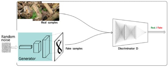
Figure 1.
The steps for GAN.
The conventional generative models use different forms of probability density function to approximate the distribution [9]. However, it cannot perform well on complex distributions. Those models may include the infinite Gaussian mixture models (GMM) [10], the hidden naive Bayes model (NBM) [10], and the hidden Markov models (HMM) [11]. An auto-encoder has a structure similar to multi-layer perceptron (MLP) which has the primary difference when using an unsupervised data for the number of neurons in the output layer is equal to the number of inputs [12]. In addition, a variation auto-encoder (VAE) learns the basic probability distribution and generates a new sample for Bayesian inference by maximizing the lower bound of the log-likelihood. In contrast, generative adversarial networks learn data distributions through the adversarial training process by the game theory instead of maximizing the likelihood. Therefore, the GAN approach has several advantages over VAE-based models: (1) the capability to learn and simulate the complex data distributions and (2) the ability to efficiently create brilliant and vividly.
The goal of this study is to identify the driftwood of the study area through image data by the GAN approach. Then, the parallel data also use the texture information to improve the classification outcomes. Due to the driftwood having an irregular shape, it should need some texture information to reinforce the content of data to reach a better classification performance. The data and methods of GAN will be introduced in the following section.
2. Data Collection and Methods
2.1. Data
The first type of image to use is the original image (B, G, R, and IR) taken from the UAV (Unmanned Aerial Vehicle) with 20 cm × 20 cm image resolution. The entire area consists of 5975 × 2075 pixels. The second type of image used requires applying the gray image with optimized texture. We adopted the texture information listed in Table 1. Figure 2 presents the study steps for analysis. We selected 134 training samples for the following categories: driftwood, grass, rock, gravel, tree, road, and seawater, respectively. In addition, we also take 58 testing samples for the above categories. This ratio is designed to satisfy the ratio of 7 to 3 of training/testing for most of the classification theory. We used ADAM (Adaptive Moment Estimation [13], which is a popular optimization algorithm used in training deep learning models) and SGD (stochastic gradient descent, which is an iterative optimization algorithm that aims to minimize a given loss function by updating the parameters of model by using the gradients of the loss with respect to those parameters) as the optimizer for showing the difference as the iteration of computation [14]. Then, RELU (Rectified Linear Unit is a simple effective non-linear function that introduces non-linearity into the neural network) is used as an activating function for the network’s internal transformation of deep learning. In pixel-based image classification, the texture information is an essential material for improving the accuracy outcomes. Hence, we employed four valuable texture indicators in Table 1, referring to Wan and Lei [1]. The texture image contains spatial distribution-related information which can successfully increase image classification. In some cases, the appropriate selection of texture images can increase classification accuracy. The following four types of texture information are used: (1) Homogeneity, (2) Contrast, (3) Dissimilarity, and (4) Entropy.

Table 1.
Texture indices for ancillary information of GAN.
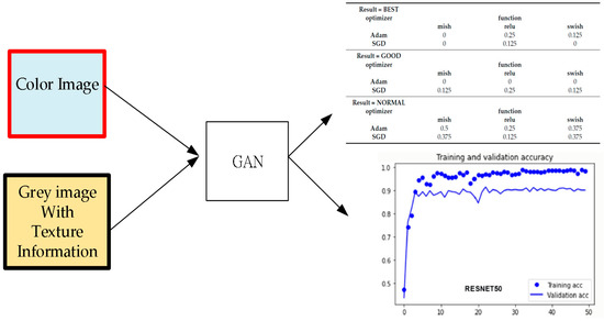
Figure 2.
Study plan. Note: acc is Accuracy, RESNET50 is RESNET with 50 epochs of iteration.
In the study, the image fusion of the gray level of pixels in texture information follows the following equation of Open CV [15]:
The entire study contains four parts. The first part discusses the background of the GAN and classifies the driftwood in the coastal area that may face the problem. The second part introduces the data we obtained and the format of it. The third part presents how the GAN operates for this study plan. The last part shows the results for the classification prediction of GAN.
2.2. Methods
Generative Adversarial Networks (GANs) are generally considered as an unsupervised learning model. It was introduced by Ian J. Goodfellow in 2014 [2,3]. GANs are the ideal of a basic system of two rival neural network models. They contend with each other and are able to simulate a series of variations within a dataset to analyze them. The generative network can create candidates while the discriminative network is used to evaluate them. The contest operates in terms of data distribution. The generative network learns the implicit mapping rules from a latent space to a data distribution to operate the discriminative network, which can distinguish candidates produced by the generator from the true data distribution. The generative network’s training objective is to “fool” the discriminator network by producing novel candidates that the discriminator thinks are not synthesized.
Generative Adversarial Networks (GANs) can be divided into three parts:
- Generative: It learns a generative model to describes how data are generated considering a probabilistic model.
- Adversarial: The training data of a model are made by an adversarial setting.
- Networks: Use deep neural networks as artificial intelligence (AI) algorithms for training progress.
We proposed a set of deep-learning-based GAN (Generative Adversarial Network)-structured labeled data to detect the area of driftwood on the seashore. Figure 3 shows the model for GAN for handling the picture-based image data for classification analysis.
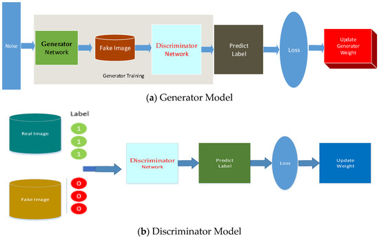
Figure 3.
Generator and discriminator models.
Step 1: The user labels render only a few amounts of few defective driftwood images and save the labeled images into our system.
Step 2: The module produces a defect-sensitive model through the GAN technique.
Step 3: A series of prototype images are used as base images to be taken by the UAV.
Step 4: The generative network creates candidates with respect to the discriminative network and evaluates them [16]. The contest follows in terms of data distribution. Generally, the generative network is designed to learn the map from a latent space to a data distribution when the discriminative network discriminates candidates produced by the generator from the true data distribution. The generative network’s training goal is to increase the error rate of the discriminative network.
Step 5: A given dataset serves as the initial training data for the discriminator. Training progress concerns presenting them from the training dataset until it approaches an acceptable level of accuracy. The generator trains the data by considering whether it succeeds in fooling the discriminator. Typically, the generator is produced by randomly input sampled data through a given latent space [17,18,19].
Afterwards, we step-by-step plan the entire study to four stems.
- (a)
- The Generator Model
The generator model generates a set of samples in the domain using a set of input random vectors. A Gaussian distribution can be typically utilized to generate the vector, which is then used as a seed for the generative process. A compressed representation of the data distribution will be formed after training when points in this multidimensional vector space will be assigned to points in the issue domain. This vector space is also known as a latent space or a vector space made up of latent variables. Latent variables, often known as hidden variables, are factors that are significant for a domain but cannot be seen directly [20,21,22].
- (b)
- The Discriminator Model
The discriminator model forecasts a series of binary class labels of actual or fake (created), using the sample from the domain as input (real or generated). In other words, the training dataset contains the actual example. The generator model outputs the created examples. An ordinary (and well-known) classification model serves as the discriminator [23]. The discriminator model is eliminated during the training progress, since we are more interested in the generator. Generally speaking, the generator is adaptable because it has mastered the art of successfully extracting features from instances in the issue area. With the same or similar input data, some or all of the feature extraction layers can be employed in transfer learning applications [24,25,26].
- (c)
- Generation of training samples and testing samples
There are 7 categories of images made of 28 × 28 pixels, which are located at the northeast of the coast of Taiwan. This is the training sample of the study area. Figure 4 shows all the categories and distributions for the training samples and locations for testing samples.
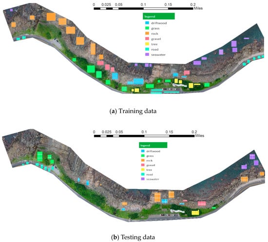
Figure 4.
Sampling of picture of the coastal area: (a) training data region, (b) testing data region.
- (d)
- Generate the confusion matrix and thematic map for verification
The confusion matrix uses the testing samples to ensure our two approaches are valid. The first approach considered using the original bands for GAN. The second approach applied the texture information with the original band for GAN. The results for the confusion matrix and thematic map are both rationally presented.
3. Results
3.1. The Post-Progress for GAN
The previous preliminary steps for GAN are defined architecture, data preparation, initializing the networks, and training loop. Then, the dropout and training are incorporated into the second stage of the generator and discriminator networks:
- (1)
- Dropout in discriminator: During training, we applied dropout to the discriminator’s hidden layers. For example, you can set a dropout rate of 0.5, meaning 50% of the neurons are randomly deactivated during each forward and backward pass.
- (2)
- Training the discriminator: We sampled a batch of real data from the dataset and generated a batch of fake data using the generator. Then, we trained the discriminator with the real and fake data batches: We computed the discriminator loss based on how well it distinguishes real from fake data. Then, we updated the discriminator’s weights and biases using backpropagation.
- (3)
- Dropout in generator: During training, we applied dropout to the generator’s hidden layers (if necessary). See Figure 5.
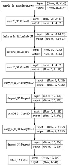 Figure 5. Steps for dropout and used active function.
 - (4)
- Training the generator: We generated a new batch of fake data using the generator. Then, we trained the generator to “fool” the discriminator. We computed the generator loss based on the discriminator’s response to the generated data. Afterwards, we updated the generator’s weights and biases using backpropagation.
The final step is used to build the ending criteria:
- (i)
- Alternating training: Step 2 and Step 4 are used to exchange information between each other.
- (ii)
- Loss function: We used appropriate loss functions, such as binary cross-entropy, to guide the training of both the discriminator and the generator.
- (iii)
- Hyperparameter tuning: Usually, we experiment with different learning rates, batch sizes, dropout rates, and architectures to optimize GAN training.
- (iv)
- Stopping criteria: We decided on a stopping criterion based on the performance of the discriminator and generator. The latter will discuss the outcomes of accuracy.
3.2. Epoch for Accuracy
Generally, a neural network is a supervised machine learning algorithm that is typically used to solve classification problems. However, using neural networks for machine learning has its advantages and disadvantages. Developing a neural network model involves addressing various architecture-related issues [27,28]. It usually depends on the complexity of the problem and the available data; we can train neural networks of different sizes and depths. It has to be noticed that most of the neural network system requires iterations (recorded as epoch) to present the convergence speed of learning [29]. Additionally, we need to preprocess our input features, initialize the weights, add bias if necessary, and select appropriate activation functions [30,31].
The accuracy and loss values are the way to observe the convergence and prediction for each epoch, which are plotted in Figure 6a,b. The GAN has two types of loss functions: one for generator training and one for discriminator training. Both the generator and discriminator losses are calculated from a single measure of distance between the probability distributions of functions. However, during generator training, we drop the term in the distance measurement that reflects the distribution of the real data and focuses only on the term that reflects the distribution of the fake data. Figure 6a presents the percentage errors of the generator on the y-axis, while Figure 6b presents the percentage errors of the discriminator. The red bars represent the accuracy (in %), and the blue lines represent the error rates. The focus of the observations was on the convergence of the last 600 epochs. The generator randomly produced many samples, resulting in a significant deviation in the loss.
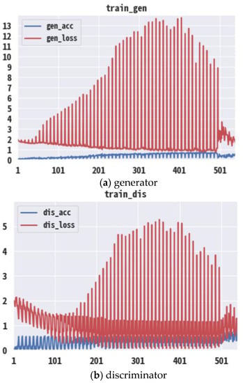
Figure 6.
The outcomes of accuracy rate and prediction loss. Note: The x-axis is the number of epochs; the y-axis is the value of loss (for red) and accuracy (for blue).
3.3. Confusion Matrix
Confusion matrix on images from GAN of datasets without any pre-processing on 28 × 28 pixels. The study plans to classify seven categories as driftwood, grass, rock, gravel, tree, road, and seawater. Through the GAN approach, the prediction accuracy is about 0.7. This is because most of the driftwoods are irregular in shape, which makes it very hard to identify their appearance by GAN with raw image material. Current advances for Generative Adversarial Networks (GANs) have create a series of realistic-looking digital images that create a major challenge to the detection by the computer model. In addition, we also use the selected texture information as material to attain the accuracy of the prediction of the confusion matrix.
It has to be noticed that the driftwoods in Figure 7a are all misclassified as rock. This is due to the driftwoods being irregular without any certain shape. With applying useful texture information (Table 1), the driftwood will successfully be detected by GAN. Thus, it can be concluded that texture information is a crucial material for picture-based deep learning classifiers.
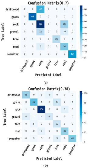
Figure 7.
The confusion matrix of two different types of image material. (a) The confusion matrix of color image with GAN; (b) The confusion matrix of gray image by texture information with GAN.
3.4. Prediction for Thematic Map
A thematic map displays the geographic pattern of a specific category (thematic) in a geographic area. This often contains the use of different colors and map symbols to present the selected target category of geographic features which are determined by a given classifier.
Driftwood is a precious material in the coastal area of Taiwan. If a UAV can take some images or pictures to quickly observe the locations of driftwood, it can save a lot of time. However, generating a thematic map can be challenging with a picture-based deep-learning approach; thus, we have to opt to use square blocks to present it. The left side of the blocks represents the real categories, while the right side shows the predicted categories generated by the GAN. We also overlapped the prediction category on the top of the ground-truth area. Figure 8a,c show the prediction by a color image, and Figure 8b,d show the prediction of the gray image with texture information. The main finding is that in Figure 8c,d, the driftwoods are being successfully predicted.
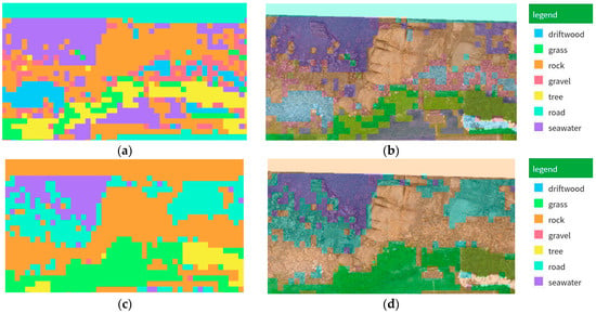
Figure 8.
The original bands for plotting thematic map. (a) Prediction for original bands; (b) Overlap (a) to the ground truth area; (c) Prediction for employed texture information; (d) Overlap (c) to the ground truth area.
4. Conclusions
Driftwood has always been regarded as a precious natural asset in Taiwan. The locations and distributions of driftwoods are difficult for detecting by spatial technology combing with deep learning approaches. However, the essential idea of a GAN derives from the “indirect” training through the discriminator, another neural network that can tell how “realistic” the input seems, which itself is also being updated automatically. With the rapid growth in deep learning approaches, the studies of computing digital images for many computer vision assessments have played an important role in recent years due to different algorithms’ extraordinary performance and the availability of large amounts of data. If one can select a proper training data set, the model learns through those data and then generates new predictions with testing samples for classification. For instance, a GAN model train in pictures look at least superficially precise to human observers in which they may have many realistic attributes. The originally proposed as a form of a generative model for unsupervised learning, then, it directly applied raw data (e.g., an R+G+B + IR image) and eliminated the needs for domain features. The preliminary study finds there are two approaches to obtaining the regional picture to attain the image classification for driftwood. The first one is to use an R+G+B + IR image. Alternatively, we also can use the gray image with texture information to attain the thematic map. The accuracy of their results is outlined below:
- (a)
- Original RGB + IR image has about 70% overall classification outcomes. All the driftwood accuracy is misclassified. But a big amount of rock was misclassified, reducing the producer accuracy.
- (b)
- The texture gray-based image has about 78% overall classification outcomes. But a large amount of grass has been misclassified to the tree, reducing the producer accuracy. The driftwood has about 79.5% producer accuracy.
Author Contributions
Conceptualization, M.-L.Y. and S.W.; Methodology, S.W. and M.-L.Y.; Validation, S.W. and M.-L.Y.; Programing H.-L.M.; Formal analysis and investigation H.-L.M. and S.W.; Writing—original draft preparation, S.W.; Writing—review and editing, S.W., H.-L.M. and T.-Y.C. All authors have read and agreed to the published version of the manuscript.
Funding
This research was funded by grant number MOST 110-2121-M-275-001 and NSTC 112-2121-M-275-001.
Data Availability Statement
The data provider is the GIS center Taiwan.
Acknowledgments
The authors expressed their gratitude for the Ministry of Science and Technology (MOST 110-2121-M-275-001) for sponsoring this work.
Conflicts of Interest
The authors declare no conflict of interest.
References
- Wan, S.; Lei, T.C. A development of a robust machine for removing Irregular noise with the intelligent system of auto-encoder for image classification of coastal waste. Environments 2022, 9, 114. [Google Scholar] [CrossRef]
- Kwak, G.H.; Park, N.W. Impact of texture information on crop classification with machine learning and UAV images. Appl. Sci. 2019, 9, 643. [Google Scholar] [CrossRef]
- Goodfellow, I.; Pouget-Abadie, J.; Mirza, M.; Xu, B.; Warde-Farley, D.; Ozair, S.; Bengio, Y. Generative adversarial networks. Commun. ACM 2020, 63, 139–144. [Google Scholar] [CrossRef]
- Gui, J.; Sun, Z.; Wen, Y.; Tao, D.; Ye, J. A Review on Generative Adversarial Networks: Algorithms, Theory, and Applications. IEEE Trans. Knowl. Data Eng. 2023, 35, 3313–3332. [Google Scholar] [CrossRef]
- Radford, A.; Metz, L.; Chintala, S. Unsupervised representation learning with deep convolutional generative adversarial networks. arXiv 2015, arXiv:1511.06434. [Google Scholar]
- Luc, P.; Couprie, C.; Chintala, S.; Verbeek, J. Semantic segmentation using adversarial networks. arXiv 2016, arXiv:1611.08408. [Google Scholar]
- Chen, Y.; Lin, Z.; Zhao, X.; Wang, G.; Gu, Y. Deep learning-based classification of hyperspectral data. IEEE J. Sel. Top. Appl. Earth Obs. Remote Sens. 2014, 7, 2094–2107. [Google Scholar] [CrossRef]
- Wan, S. A spatial decision support system for extracting the core factors and thresholds for landslide susceptibility map. Eng. Geol. 2009, 108, 237–251. [Google Scholar] [CrossRef]
- Lu, X.; Matsuda, S.; Hori, C.; Kashioka, H. Speech restoration based on deep learning Auto-encoder with layer-wised pretraining. In Proceedings of the Thirteenth Annual Conference of the International Speech Communication Association, Portland, OR, USA, 9–13 September 2012. [Google Scholar]
- Kudo, Y.; Aoki, Y. Dilated convolutions for image classification and object localization. In Proceedings of the 2017 Fifteenth IAPR International Conference on Machine Vision Applications (MVA), Nagoya, Japan, 8–12 May 2017; pp. 452–455. [Google Scholar]
- Chang, S.H.; Wan, S. A novel study on ant-based clustering for paddy rice image classification. Arab. J. Geosci. 2015, 8, 6305–6316. [Google Scholar] [CrossRef]
- Pham, D.T.; Sagiroglu, S. Training multilayered perceptrons for pattern recognition: A comparative study of four training algorithms. Int. J. Mach. Tools Manuf. 2001, 41, 419–430. [Google Scholar] [CrossRef]
- Pang, Y.; Sun, M.; Jiang, X. Convolution in convolution for network in network. IEEE Trans. Neural Netw. Learn. Syst. 2018, 29, 1587–1597. [Google Scholar] [CrossRef]
- Odena, A.; Olah, C.; Shlens, J. Conditional image synthesis with auxiliary classifier gans. In Proceedings of the 34th International Conference on Machine Learning, Sydney, Australia, 6–11 August 2017; Volume 70, pp. 2642–2651. [Google Scholar]
- Available online: https://docs.opencv.org/3.4/de/d25/imgproc_color_conversions.html (accessed on 11 June 2021).
- Armanious, K.; Hepp, T.; Küstner, T.; Dittmann, H.; Nikolaou, K.; La Fougère, C.; Yang, B.; Gatidis, S. Independent attenuation correction of whole body [18F] FDG-PET using a deep learning approach with Generative Adversarial Networks. EJNMMI Res. 2020, 10, 53. [Google Scholar] [CrossRef]
- Mao, X.; Li, Q.; Xie, H. Aligngan: Learning to align cross-domain images with conditional generative adversarial networks. arXiv 2017, arXiv:1707.01400. [Google Scholar]
- Schlegl, T.; Seeböck, P.; Waldstein, S.M.; Schmidt-Erfurth, U.; Langs, G. Unsupervised anomaly detection with generative adversarial networks to guide marker discovery. In Proceedings of the International Conference on Information Processing in Medical Imaging, Boone, NC, USA, 25–30 June 2017; Springer: Berlin/Heidelberg, Germany, 2017; pp. 146–157. [Google Scholar]
- Hsu, C.C.; Lee, C.Y.; Zhuang, Y.X. Learning to Detect Fake Face Images in the Wild. In Proceedings of the 2018 International Symposium on Computer, Consumer and Control (IS3C), Taichung, Taiwan, 6–8 December 2018; IEEE: New York City, NY, USA, 2018; pp. 388–391. [Google Scholar]
- Wu, Q.; Wang, P.; Shen, C.; Reid, I.; van den Hengel, A. Are you talking to me? Reasoned visual dialog generation through adversarial learning. In Proceedings of the IEEE Conference on Computer Vision and Pattern Recognition, Salt Lake City, UT, USA, 18–23 June 2018; pp. 6106–6115. [Google Scholar]
- Joo, D.; Kim, D.; Kim, J. Generating a Fusion Image: One’s Identity and Another’s Shape. In Proceedings of the IEEE Conference on Computer Vision and Pattern Recognition, Salt Lake City, UT, USA, 18–23 June 2018; pp. 1635–1643. [Google Scholar]
- Reed, S.E.; Akata, Z.; Mohan, S.; Tenka, S.; Schiele, B.; Lee, H. Learning what and where to draw. In Advances in Neural Information Processing Systems; MIT Press: Cambridge, MA, USA, 2016; pp. 217–225. [Google Scholar]
- Karpathy Atoderici, G. Large-scale video classification with convolutional neural networks. In Proceedings of the IEEE Computer Society Conference on Computer Vision and Pattern Recognition, Nanjing, China, 28–30 July 2014; pp. 1725–1732. [Google Scholar] [CrossRef]
- Krizhevsky Ahinton, G. Neural ImageNet Classification with Deep Convolutional Neural Networks. Inf. Process. Syst. 2012, 25, 1–9. [Google Scholar] [CrossRef]
- Gu, J.; Wang, Z.; Kuen, J.; Ma, L.; Shahroudy, A.; Shuai, B.; Liu, T.; Wang, X.; Wang, G.; Cai, J.; et al. Recent advances in convolutional neural networks. Pattern Recognit. 2018, 77, 354–377. [Google Scholar] [CrossRef]
- Badrinarayanan, V.; Kendall, A.; Cipolla, R. SegNet: A Deep Convolutional Encoder-Decoder Architecture for Image Segmentation. IEEE Trans. Pattern Anal. Mach. Intell. 2017, 39, 2481–2495. [Google Scholar] [CrossRef] [PubMed]
- Lange, S.; Riedmiller, M. Deep auto-encoder neural networks in reinforcement learning. In Proceedings of the International Joint Conference on Neural Networks, Barcelona, Spain, 18–23 July 2010. [Google Scholar] [CrossRef]
- Espindola, G.M.; Camara, G.; Reis, I.A.; Bins, L.S.; Monteiro, A.M. Parameter selection for region-growing image segmentation algorithms using spatial autocorrelation. Int. J. Remote Sens. 2006, 27, 3035–3040. [Google Scholar] [CrossRef]
- Du, P.; Tan, K.; Xing, X. A Novel Binary Tree Support Vector Machine for Hyperspectral Remote Sensing Image Classification. Opt. Commun. 2012, 285, 3054–3060. [Google Scholar] [CrossRef]
- Chapelle, O.; Haffner, P.; Vapnik, V. Support vector machines for histogram-based image classification. IEEE Trans. Neural Netw. 1999, 10, 1055–1064. [Google Scholar] [CrossRef] [PubMed]
- Furey, T.; Cristianini, N.; Duffy, N.; Bednarski, D.; Schummer, M.; Haussler, D. Support vector machine classification and validation of cancer tissue samples using microarray expression data. Bioinformatics 2000, 16, 906–914. [Google Scholar] [CrossRef] [PubMed]
Disclaimer/Publisher’s Note: The statements, opinions and data contained in all publications are solely those of the individual author(s) and contributor(s) and not of MDPI and/or the editor(s). MDPI and/or the editor(s) disclaim responsibility for any injury to people or property resulting from any ideas, methods, instructions or products referred to in the content. |
© 2023 by the authors. Licensee MDPI, Basel, Switzerland. This article is an open access article distributed under the terms and conditions of the Creative Commons Attribution (CC BY) license (https://creativecommons.org/licenses/by/4.0/).