Review

Paleoliquefaction Studies and the Evaluation of Seismic Hazard

1
M. Tuttle & Associates, P.O. Box 345, Georgetown, ME 04548, USA
2
Lettis Consultants International, Inc., Santa Clarita, CA 91355, USA
3
Department of Geosciences, Auburn University, Auburn, AL 36849, USA
4
Civil & Environmental Engineering, Georgia Institute of Technology, 790 Atlantic Drive, Atlanta, GA 30332, USA
*
Author to whom correspondence should be addressed.
Geosciences 2019, 9(7), 311; https://doi.org/10.3390/geosciences9070311
Submission received: 7 June 2019 / Revised: 5 July 2019 / Accepted: 7 July 2019 / Published: 13 July 2019

Abstract

:
Recent and historical studies of earthquake-induced liquefaction, as well as paleoliquefaction studies, demonstrate the potential usefulness of liquefaction data in the assessment of the earthquake potential of seismic sources. Paleoliquefaction studies, along with other paleoseismology studies, supplement historical and instrumental seismicity and provide information about the long-term behavior of earthquake sources. Paleoliquefaction studies focus on soft-sediment deformation features, including sand blows and sand dikes, which result from strong ground shaking. Most paleoliquefaction studies have been conducted in intraplate geologic settings, but a few such studies have been carried out in interplate settings. Paleoliquefaction studies provide information about timing, location, magnitude, and recurrence of large paleoearthquakes, particularly those with moment magnitude, M, greater than 6 during the past 50,000 years. This review paper presents background information on earthquake-induced liquefaction and resulting soft-sediment deformation features that may be preserved in the geologic record, best practices used in paleoliquefaction studies, and application of paleoliquefaction data in earthquake source characterization. The paper concludes with two examples of regional paleoliquefaction studies—in the Charleston seismic zone and the New Madrid seismic zone in the southeastern and central United States, respectively—which contributed to seismic source models used in earthquake hazard assessment.

1. Introduction

Paleoseismology is the study of prehistoric earthquakes as preserved in the geologic record, and it improves our understanding of the long-term behavior of fault zones and seismic sources (e.g., Reference [1]). Paleoseismology is especially useful in regions where strain rates are relatively low and recurrence times of large earthquakes are longer than the historical record. In such regions, the seismicity catalog is often insufficient to characterize the expected rates of large events, a critical issue for estimating uncertainty in seismic hazard assessments.
The paleoliquefaction approach to paleoseismology focuses on soft-sediment deformation structures and related ground failures resulting from liquefaction induced by earthquakes. This field of study developed over the past 40 years and provides important information about timing, source areas, magnitudes, and recurrence times of large paleoearthquakes during the Late Quaternary. Paleoliquefaction studies are especially useful in intraplate and interplate regions where seismogenic faults may not rupture the surface or are otherwise difficult to identify [2,3]. Paleoliquefaction studies have been conducted in seismically active regions of central and eastern North America, including the New Madrid seismic zone in the central United States (US) (e.g., References [4,5,6,7,8]), the Charleston seismic zone in the southeastern US (e.g., References [9,10,11,12]), and the Charlevoix seismic zone in southeastern Canada [13], where large historical earthquakes are known to have induced liquefaction (Figure 1). They have been carried out in the Wabash Valley (e.g., References [14,15]) and the Eastern Tennessee [16] seismic zones, where only small to moderate earthquakes occurred during the historical period. In addition, paleoliquefaction studies were conducted in interplate settings like the Dominican Republic and Puerto Rico in the northeastern Caribbean and the Pacific Northwest in the US, where subduction zones and crustal faults pose a significant seismic hazard (e.g., References [3,17,18,19,20]). Paleoliquefaction studies have been conducted in a lacustrine setting in eastern Turkey [21] and a volcanic setting in southern Italy [22]. Studies focusing on soft-sediment deformation structures in lacustrine deposits were reported for southern Italy [23], Mexico [24], and Argentina [25]. Recently, several paleoliquefaction studies were carried out in the Canterbury region of New Zealand, where a system of crustal faults, some of which did not rupture the surface, produced the 2010–2011 sequence of earthquakes and caused extensive and recurrent liquefaction (e.g., References [26,27,28,29,30,31,32]).
Paleoliquefaction data were used to develop seismic source models for the US national seismic hazard maps [33,34] and for the central and eastern US (CEUS) seismic source characterization for nuclear facilities [35]. Paleoliquefaction studies, along with other paleoseismic investigations such as fault studies, supplement modern seismicity studies and provide critical information on the long-term behavior and earthquake potential of seismic sources, which is essential for probabilistic seismic hazard assessments. This review paper presents background information on earthquake-induced liquefaction and resulting soft-sediment deformation features that may be preserved in the geologic record, best practices used in paleoliquefaction studies, and application of paleoliquefaction data in earthquake source characterization.

2. Earthquake-Induced Liquefaction

The 1964 Alaska (US), 1964 Niigata (Japan), and 1967 Caracas (Venezuela), earthquakes caused catastrophic liquefaction-related failures (e.g., Reference [37]). More recent earthquakes, including the 1995 Hyogo-ken Nanbu (Japan) and 2010–2019 Canterbury (New Zealand) earthquakes also caused large economic losses due to liquefaction-related damages to the built environment (e.g., References [38,39]). These and other events spurred research in earthquake-induced liquefaction and earthquake soil dynamics in the geological and geotechnical engineering communities. Progress was made in better understanding the process of liquefaction, the conditions contributing to liquefaction, and ground motions that initiate liquefaction; however, many uncertainties remain regarding liquefaction triggering assessment, including the influence of fines and gravel content of soils, age effects on liquefaction susceptibility, the degree of saturation below the water table, and methods for predicting liquefaction triggering [40]. Readers are referred to the National Academies of Sciences [40] for a thorough review of the art and practice in the assessment of earthquake-induced liquefaction and its consequences. Aspects of earthquake-induced liquefaction especially pertinent to paleoliquefaction studies are summarized below.

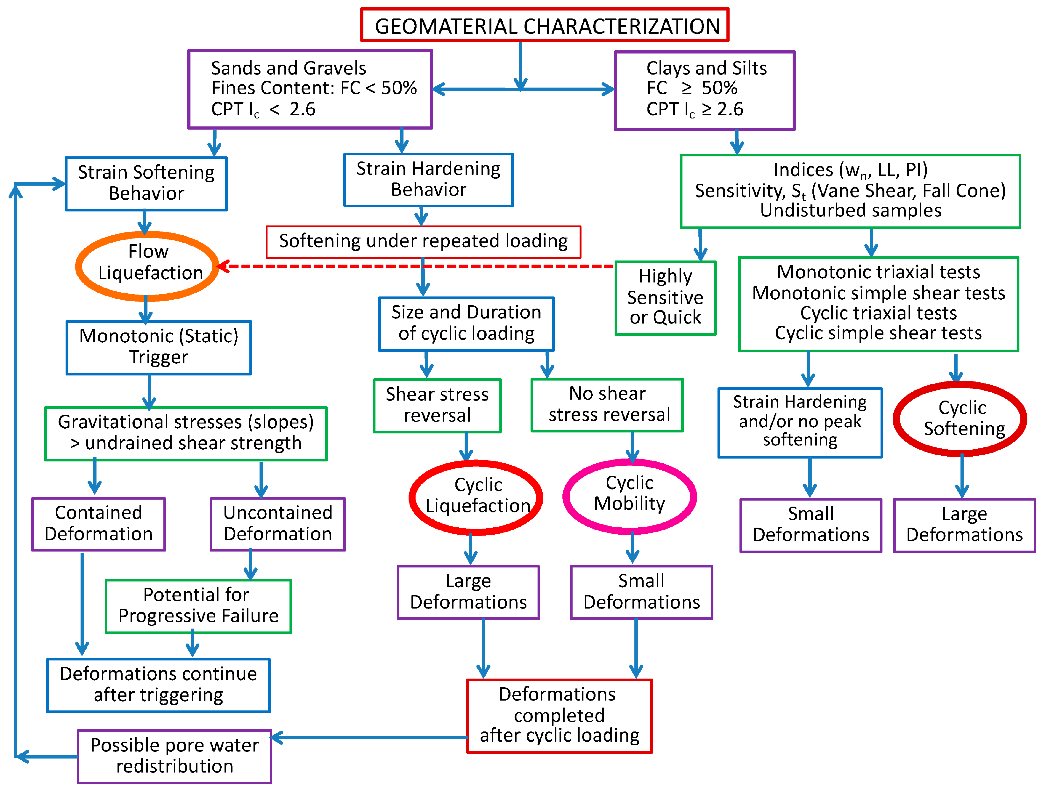
2.1. Process of Liquefaction

There are two primary types of liquefaction: (a) flow liquefaction, associated with static monotonic loading; and (b) cyclic liquefaction, caused by repeated (earthquake) loading (Figure 2 [41,42]). In cases of both cyclic and flow liquefaction, a significant loss of soil strength occurs. Cyclic liquefaction results from the accumulation of excess porewater pressure in granular soils (sands and gravels) as repeated load cycles are applied by earthquake ground motions. Flow liquefaction occurs during first-time (monotonic static) loading of unstable soils, including sands, silts, and clays.
At most documented liquefaction sites, the more common mechanism is cyclic liquefaction. Cyclic liquefaction occurs when the structure of water-saturated, loose, granular sediment breaks down due to rapidly applied and repetitive loading caused by earthquakes [37,41,42,43]. During cyclic loading, the loosely packed particles attempt to move into a denser configuration (termed contraction). During an earthquake, however, there is not enough time for the water in the pores of the sediment to be squeezed out. Instead, the water is trapped and prevents the particles from moving closer together. This is accompanied by an increase in porewater pressure that reduces the contact forces between the individual particles, thereby softening and weakening the sediment. In loose contractive sand, the development of positive porewater pressure reduces the effective stress state and, when the effective strength envelope is reached, the onset of cyclic liquefaction occurs (e.g., Reference [41]). During large earthquakes, the increase in porewater pressure can lead to upward flow of water and entrainment of sediment through the process of fluidization [43,44,45]. The upward flow of water and entrained sand can lead to the formation of liquefaction features, including sand dikes, diapirs, sills, and blows (Figure 3). These and other soft-sediment deformation structures are discussed further in Section 2.4 below. For additional information on the process of liquefaction, see References [40,41,46,47,48,49,50].

2.2. Conditions That Influence the Formation of Liquefaction Features

Earthquake-induced liquefaction features commonly form in alluvial, coastal, deltaic, and lacustrine deposits of the Holocene age (0.01 Ma to present), where sand is interbedded with silt and clay and shallow groundwater conditions prevail (e.g., References [28,29,30,31,32,52,53,54,55,56,57,58,59,60,61]). Sedimentological and hydrological conditions in these environments are conducive to the formation of liquefaction features. Liquefaction features also formed in similar deposits of the Late Pleistocene age (0.126 to 0.01 Ma) (e.g., References [13,14,52]) and as old as 200,000–240,000 years before present (BP) [61].
The physical properties of sediment that influence liquefaction susceptibility, or their tendency to liquefy during earthquakes include the size, shape, and packing arrangement of the sediment grains [37,40,49,62]. Well-rounded, well-sorted, loose to moderately loose, fine sand with a high void ratio or low relative density would be especially susceptibility to liquefaction, so long as it is saturated. Liquefaction susceptibility decreases with increasing fines content, especially fines with a high plasticity index [40,63,64,65]. Layering in sediment plays an important role in liquefaction and the formation of liquefaction features. Layers of clay or silt form impermeable barriers that prevent or retard the upward flow of water, thereby promoting the buildup of porewater pressure in underlying sandy layers (e.g., References [66,67,68]). In addition, layers of clay or silt above sandy layers can lead to the formation of a water layer, foundering of the overlying layer, and formation of sand diapirs and dikes (e.g., References [67,69]).
Aging can have a significant effect on the strength of soil and, thus, may influence its liquefaction susceptibility (e.g., References [70,71]). Due largely to aging effects, Pleistocene (2.58 to 0.01 Ma) [72] deposits tend to be less susceptible to liquefaction than Holocene (0.01 Ma to present) [72] deposits, and pre-Pleistocene (before 2.58 Ma) deposits tend to have a very low liquefaction susceptibility [54,73]. Over time, sediment consolidates, especially if buried by subsequent deposits, becoming more densely packed and less susceptible to liquefaction. In addition, cementation of sand grains by clay, calcium carbonate, and iron and manganese oxides will strengthen the sediment and reduce its liquefaction susceptibility [74]. A fluctuating water table can promote the precipitation and concentration of clays, carbonates, and oxides. On the other hand, considerable groundwater flow can flush potential cementing agents out of sandy deposits [75]. Research in the Charleston seismic zone of the southeastern US suggests that repeated liquefaction by large earthquakes every few hundred years can counter the effects of aging or “reset the clock” (e.g., References [40,76]).

2.3. Ground Motions That Cause Liquefaction

The key index parameters of ground motion include ground acceleration, ground velocity, ground displacement, and duration of ground shaking [37,77,78]. These factors, combined with the frequency characteristics of ground motion, account for the intensity of ground shaking. Characteristics of earthquake ground motions at a particular site, which may or may not suffer liquefaction, will depend on several seismological and geological factors. These factors include magnitude of the earthquake, the source mechanism of the earthquake, distance to the site from the earthquake source, directivity of seismic energy related to the direction and speed of fault rupture, characteristics of the rocks along the wave path from source to site, and local soil conditions at the site [37].
Earthquake-induced liquefaction is caused by the buildup of excess porewater pressure due to cyclic shear stresses imparted by ground motions. In particular, the amplitude of the cyclic shear stresses and the number of cycles of shearing contribute to liquefaction [37]. Maximum shear stress is related to maximum ground acceleration. The number of cycles depends on the duration of the earthquake and also, implicitly, its frequency content. Both maximum ground acceleration and duration of ground shaking generally increase with earthquake magnitude and may also increase as a result of seismotectonic setting, site conditions, and bedrock topography (i.e., basin effects) (e.g., Reference [37]).
During the 1976 M 7.5 Guatemala, 1976 M 7.6 Tangshan (China), 1978 M 6.5 Miyagiken-Oki (Japan), 1983 M 6.8 and 7.7, Nihonkai-Chuba (Japan), 1989 M 6.9 Loma Prieta (California), 2016 M 5.8 Pawnee (Oklahoma), and M 7.1 Darfield and M 6.2 Christchurch (New Zealand) earthquakes, liquefaction was triggered by peak ground accelerations (PGAs) of ≤0.1 g [26,79,80,81]. The US National Research Council judged that a typical peak ground acceleration (PGA) threshold value of liquefaction is 0.1 g and that smaller accelerations associated with long-duration earthquakes also can induce liquefaction in very susceptible soils [82]. More recently, de Magistris et al. [83] estimated a threshold value of 0.09 g based on a statistical analysis of case histories of earthquake-induced liquefaction, primarily from Japan and the US, including earthquakes ranging from M 5.9 to M 8+. The peak acceleration for triggering liquefaction ranged from 0.08 to 0.84 g, with the most cases of liquefaction between 0.16 and 0.32 g.
Liquefaction triggering is assessed by using simplified empirical models based on in situ testing (e.g., standard penetration test or SPT, cone penetration test or CPT, shear-wave velocity) to correlate penetration resistance to relative soil density [37,41,42,49,84,85,86]. From in situ measurements at sites of liquefaction and non-liquefaction, relations are developed for predicting resistance to liquefaction triggering, or the cyclic resistance ratio ( C R R ) . The simplified empirical models evaluate the seismic loading that initiates the liquefaction process. The seismic loading is characterized as the magnitude- and stress-corrected cyclic stress ratio ( C S R M , σ v ) , which is expressed as follows [87]:
C S R M , σ v =   0.65 · ( a m a x g ) · ( σ v σ v ) · r d · 1 M S F ,
where a m a x is the peak (horizontal) ground acceleration (or PGA), g is the gravitational acceleration constant ( g = 9.8 m/s2 = 32 ft/s2), σ v and σ v are the total and effective vertical stresses, respectively, r d is a stress reduction coefficient that accounts for the flexibility of the model soil column ( r d ≤ 1.0), and M S F is a magnitude scaling factor, which is a function of M and is a proxy for the duration of loading [88]). Liquefaction triggering potential is often expressed as a factor of safety against liquefaction ( F S L ) as follows:
F S L = r e s i s t a n c e l o a d i n g = C R R C S R M , σ v .
The characterization of seismic loading in terms of a m a x and M is a critical part of empirical liquefaction triggering assessment [89].

2.4. Earthquake-Induced Liquefaction Features

There is a large body of literature on earthquake-induced liquefaction features, including articles about laboratory experiments (e.g., References [90,91]), post-earthquake surveys and studies (e.g., References [6,26,27,28,29,30,31,32,52,53,58,92,93,94,95,96]), and paleoliquefaction studies (e.g., References [6,8,9,14,15,21,22,23,24,25,97,98,99]). In addition, there are reviews on earthquake-induced liquefaction features and criteria for distinguishing them from non-seismic features (e.g., References [2,23,44,51,91,97,98,99,100]). Earthquake-induced liquefaction features are also important in the assessment of intensity fields and epicentral intensity of modern and historical earthquakes [101,102,103,104]. In the environmental seismic intensity scale (ESI) based on effects of ground shaking in the natural environment, liquefaction features along with other environmental effects are used to define earthquake intensity levels IV–XII [105,106,107]. This overview is not intended as a comprehensive discussion of all the relevant literature, but rather as an introduction for new investigators to the topic, drawing on several classic studies, our own experience, and several recent studies that advanced the field of study.
As described above in Section 2.1, strong ground shaking can induce liquefaction and fluidization of water-saturated, loose, sandy sediment, and it can lead to the formation of liquefaction features. From a geological perspective, deformation of unconsolidated sand is related to a trigger (groundwater movements, wave action, and seismic shaking), a deformation mechanism (liquefaction and fluidization), and a driving force (gravitational body force, unevenly distributed loads, unstable density gradients, and shear forces) [44]. Seismic shaking is the likely trigger for regionally extensive liquefaction and can result in the formation of sand dikes and sand blows if fluidization is involved. In addition, dish structures, load casts, pseudonodules, and ball-and-pillow structures can form in muddy and sandy sediments in response to seismic shaking; however, these features may also form as the result of other triggers. Many of the liquefaction features that are observed following earthquakes were reproduced during laboratory experiments, including sand blows with a central crater and a thin surface coating of finer sand, and loss of stratification in the feeder area or source zone [91].
Earthquake-induced liquefaction features can be divided into two categories: (1) features related to deformation extending beyond the layer that liquefies; and (2) features related to deformation within the sedimentary layer that liquefies. Features that extend beyond the liquefied layer include intrusive dikes, sills, and diapirs, and extrusive sand blows or volcanoes (e.g., References [6,21,22,23,24,26,28,29,30,31,92,100,108,109]). Features that form within the liquefied layer include disturbed bedding, dish structures, ball-and-pillow structures, load casts and related folds, pseudonodules, convolute bedding and lamination, and folds related to slumping (e.g., References [21,22,23,24,25,32,44,54,91,97,98,99,100,110,111]).

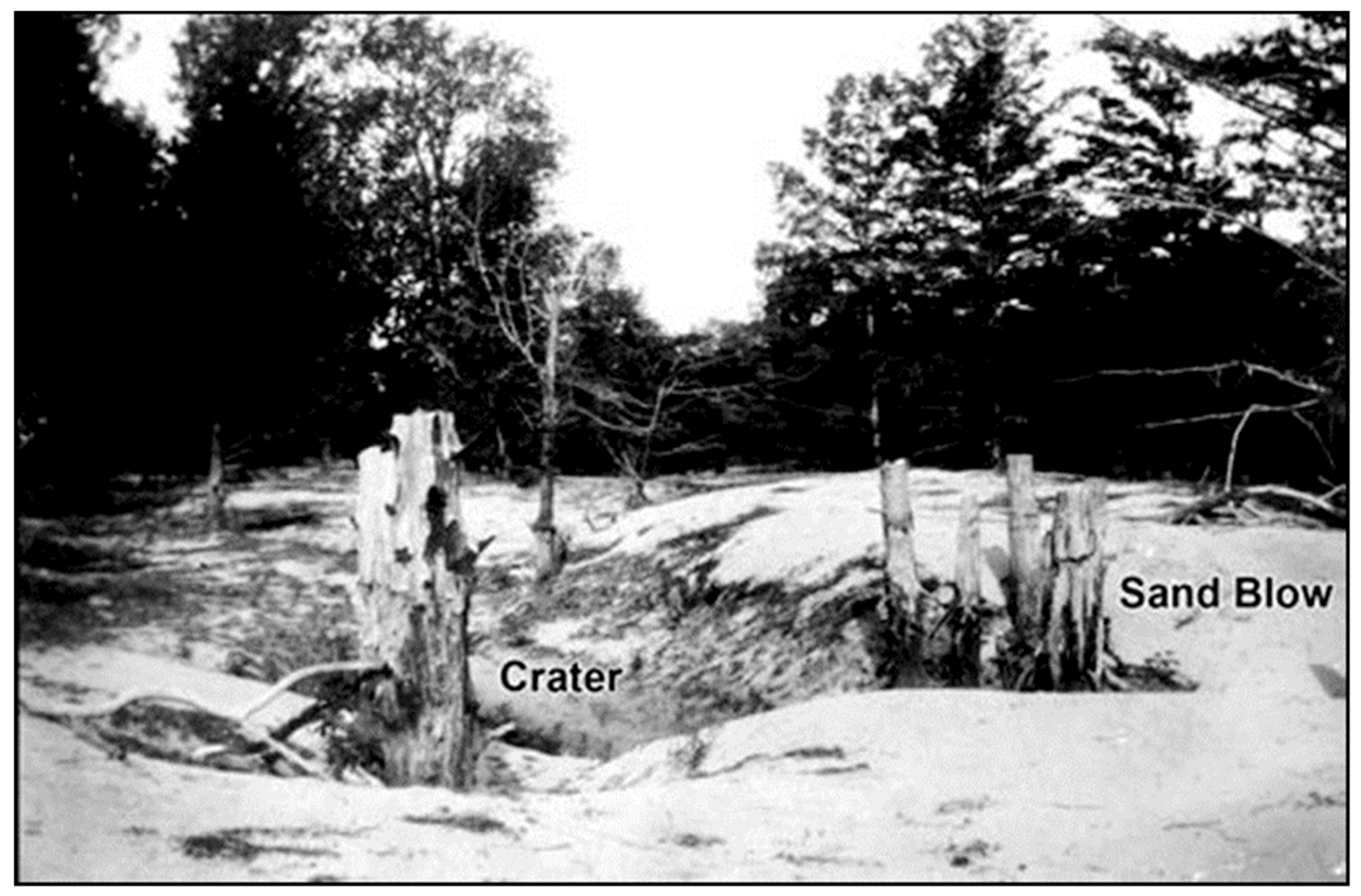
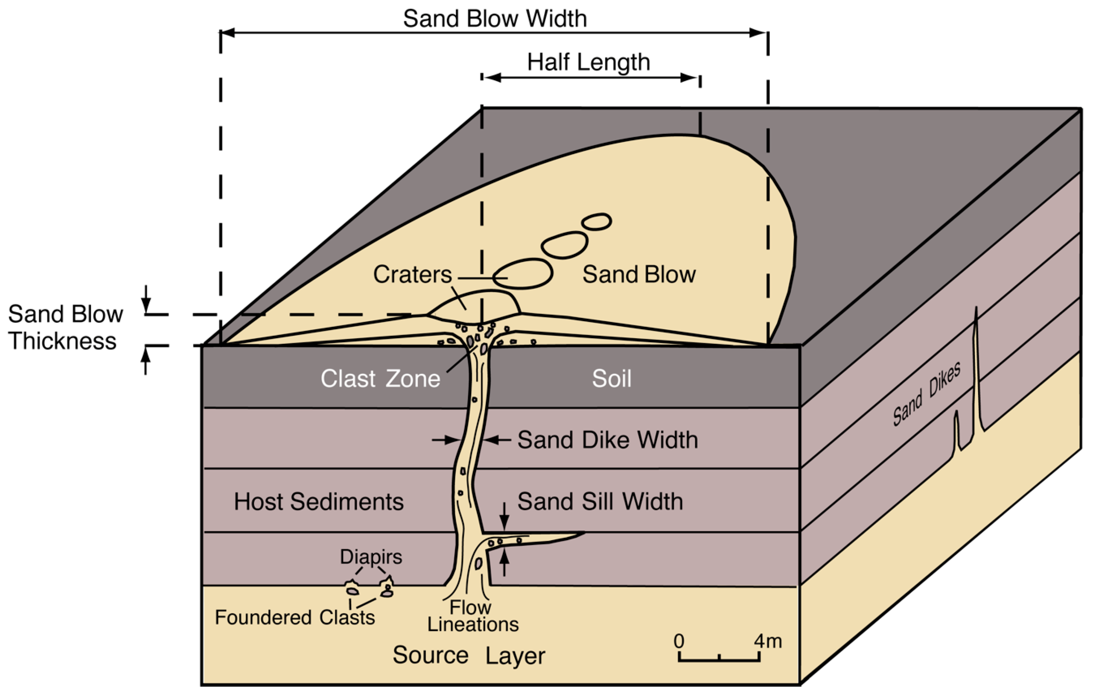
2.4.1. Blows, Dikes, Sills, and Diapirs

Sand blows result from venting of water and entrained sediment onto the ground surface at the time of the earthquake, or soon thereafter in cases of delayed effects (Figure 3, Figure 4 and Figure 5; e.g., References [51,92,99,100]). Sand blows are also called sand volcanoes because they resemble small volcanic cones, some with small craters at the surface, aligned along ground fissures. The opening at the ground surface through which the slurry of water and sediment flows is referred to as the vent. As vented water flows across the ground surface, the entrained sediment is deposited to form constructional cones or to fill topographically low or subsided areas (see photographs of sand blows that formed during the 2010–2011 Canterbury (New Zealand) earthquake sequence in the Supplementary Materials of Reference [30] and during the 2012 Emilia (Italy) earthquake sequence in Reference [112]. In plan view, the shape of a sand blow is related to the shape of the conduit through which the slurry of water and sand vented. Linear to elliptical blows result from venting through fissures [26,28,30,69,92,95]. Circular blows result from venting through tubular-shaped conduits such as root casts (e.g., Reference [113]).
Generally, sand blows are thicker and coarser-grained above the vent area and thin and fine away from the vent [6,8]. Several investigators noted that some sand blows also fine upward and are capped by silt or clay (e.g., Reference [22]), including depositional units of compound sand blows resulting from multiple earthquakes in a sequence (e.g., References [6,7,8,26,30,92]. For example, compound sand blows that formed during the 2010–2011 Canterbury (New Zealand) earthquake sequence were composed of multiple fining-upward units capped by silt drapes (Figure 4 [26,30]). Each of these fining-upward units formed during a different earthquake in the sequence. In the New Madrid seismic zone of the central US, compound sand blows that formed during the 1811–1812 earthquake sequence, as well as paleo-sand blows in the region, are composed of several depositional units that generally fine upward and are capped by silt or clay layers (Figure 5 [6,7,8]). The silt and clay layers capping the sandy units are thought to be related to low flow velocity during the waning stage of venting and, in some locations, to settling of fines out of standing water following an event.
Sand blows that formed during a single event, involving ground oscillation and pulsing of vented water and sediment, should not be confused with compound sand blows (e.g., References [58,114]). These single-event sand blows are composed of multiple sand layers that are not capped by silt or clay.
Craters form in the surface of the sand blow above the most recently active vents. Following an event, the craters are often coated with silt or clay (see examples of craters in sand blows that formed during the 2010–2011 Canterbury earthquake sequence in the Supplementary Materials of Reference [30]) and are eventually filled with wind- and water-borne sediment [92]. It was also noted that sand blows may contain clasts of the underlying deposits through which the slurry of water and sand flowed [6,8,92]. The clasts tend to be larger and more abundant in close proximity to the vent. In cases of compound sand blows that formed as a result of recurrent liquefaction, clasts are often more abundant in the lowest and earliest unit to be deposited (Figure 4 and Figure 5). The sedimentological characteristics of sand blows vary from site to site and region to region and likely depend on a number of factors such as grain-size distribution of the source bed, the flow rate and duration of venting water and entrained sediment, and variations in the flow rate related to ground oscillation and pulsing (e.g., References [5,77,92]). In cases where a large volume of subsurface sediment vented to the surface or where lateral spreading or faulting occurred, the soil horizon buried beneath the blow may dip toward the vent or be displaced downward across the vent (Figure 5 [22,69]).
Sand-blow craters that formed in the ground surface were studied in the Charleston seismic zone of the southeastern US [10,109]. Vented sediment, including clasts of soil, was deposited around the crater rims and in the base of the craters. Over time, the craters filled with reworked sand-blow deposits, slack-water deposits, and organic material [10,109]. Sand-blow craters were studied during the post-earthquake survey of the M 7.7 Bhuj (India) earthquake [58]. In at least one location, a sand-blow crater was formed by explosive deformation. Crater formation with forceful ejection of soil clasts post-date the vented sand and silt surrounding the crater, suggesting that explosive ground deformation resulted from delayed effects of soil liquefaction [115].
Sand dikes are sheet-like or tabular-shaped intrusive bodies that crosscut bedding in the host deposits (Figure 5a and Figure 6 [51,92,99,100]). Dikes usually have well-defined margins and can be differentiated from the host deposit by differences in grain size and weathering characteristics. Dikes typically originate in a layer of sandy sediment (i.e., the source layer) and are composed of sediment derived from the source layer (Figure 6). The dikes may contain clasts of the intruded host deposits and exhibit flow structure or lineations. They often become narrower and more fine-grained up section, and sometimes branch upward. Dikes may pinch out or terminate within the stratigraphic section or extend through the entire section to the ground surface. Tree root casts, animal burrows, desiccation cracks, and other voids or weak spots near the ground surface can be utilized as pathways to the surface (e.g., References [5,20,113]). Sand diapirs are similar to dikes but are relatively small intrusions of sediment extending from the layer that liquefied into the base of the overlying layer (e.g., Reference [13]). In contrast to dikes and diapirs, sills are intruded parallel to bedding of host deposits and usually take the form of lenses intruded below low-permeability layers (Figure 3 and Figure 6). The source layer of dikes, diapirs, and sills may contain foundered clasts of the overlying layer and exhibit deformation structures related to liquefaction and fluidization, such as disturbed bedding, dish structures, ball-and-pillow structures, load casts and related folds, and flow structure or lineations (e.g., References [5,13,22,97]). Alternatively, the source layer may be massive if bedding is completely destroyed.

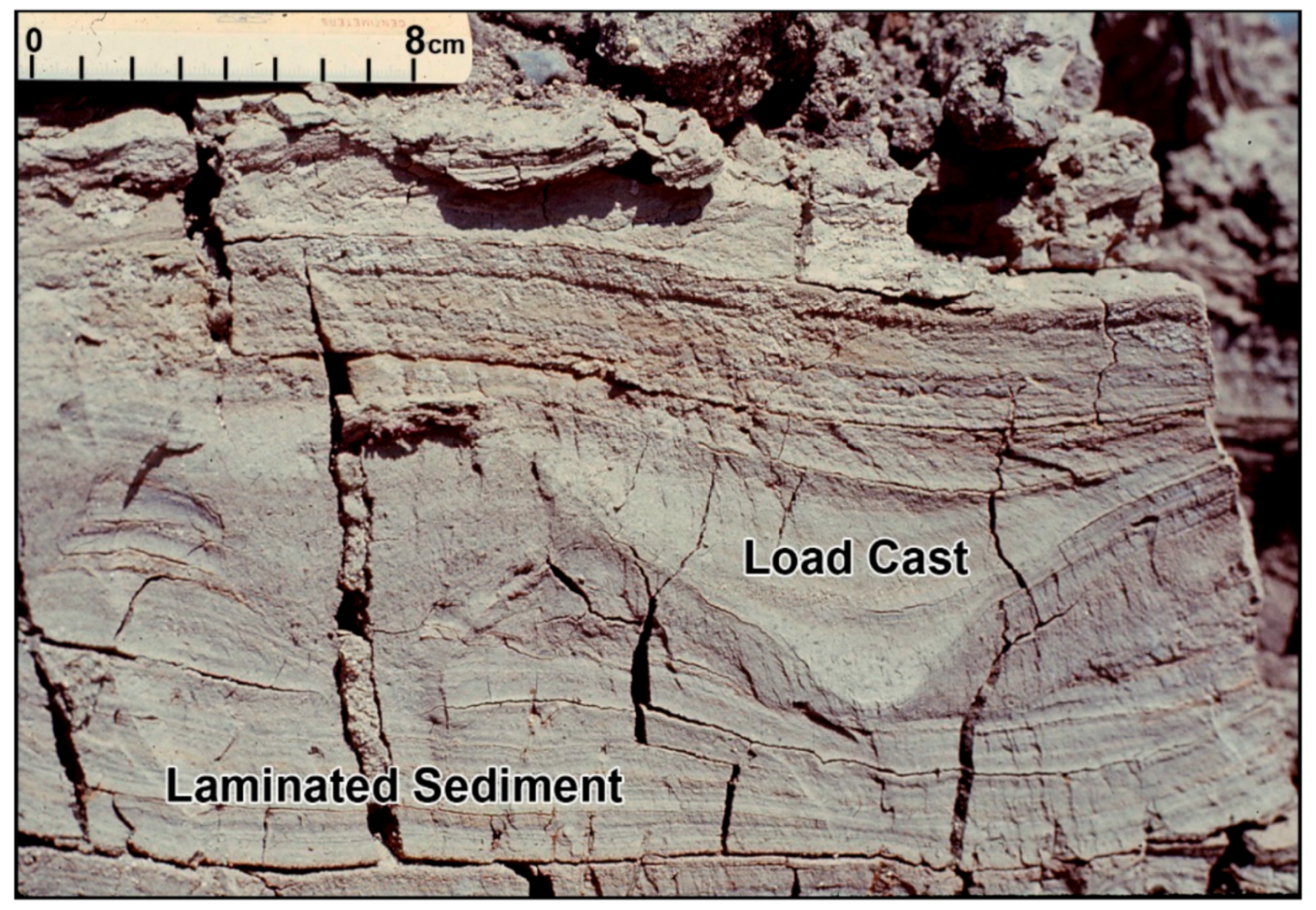
2.4.2. Soft-Sediment Deformation Structures within the Layer That Liquefied

Deformation structures within the layers that liquefied include disturbed bedding, dish structures, ball-and-pillow structures, load casts and related folds, pseudonodules, convolute bedding and lamination, and folds related to slumping (e.g., References [5,13,22,24,25,32,44,54,91,97,98,99,111,117]). In a review of the physical conditions under which soft-sediment deformation occurs, Owen [44] concluded that dish structures, load casts, pseudonodules, and ball-and-pillow structures can form in muddy and sandy sediments in response to seismic shaking, but that these features may also form as the result of other triggers. Sims [97], who pioneered the use of these types of features in paleoliquefaction studies, developed recognition criteria by studying earthquake-induced structures that formed in different environments during modern and historical earthquakes. It was noted that these liquefaction features typically form in interbedded fine- and coarse-grained deposits close to the sediment-water interface as a result of bearing strength failure due to liquefaction of the coarse-grained layers. In a more recent review, Sims [98] provided a detailed discussion of the characteristics of liquefaction features and the conditions under which these features form. In the case of load casts, fine-grained layers sag into the liquefied coarse-grained layer but without completely detaching (Figure 7). If the sagging layers detach, convolute laminations and ball-and-pillow structures form as they sink into the liquefied coarse-grained layer. Pseudonodules form when the coarse-grained layer separates into domains or irregular masses. Disturbed bedding, dish structures, and foundered clasts were also described in source layers of sand dikes and sand blows that formed during earthquakes (e.g., References [5,13,117]). In his early research, Sims [53] found that load casts form at lower modified Mercalli intensities of about VI, whereas convolute laminations and pseudonodules form at higher intensities of VIII–IX. Therefore, the occurrence of the different types of strata-bound liquefaction features may help constrain the locations and magnitudes of paleoearthquakes.
Given that strata-bound soft-sediment deformation can form as a result of a variety of triggers, it may be best to use these structures in combination with sand dikes and sand blows [13,110]. A recent study by Uner [21] was a good example of this approach. In this study, fluid-escape structures, including sand volcanoes, flame structures, and dish and pillar structures, were found in combination with disturbed layers, ball-and-pillow structures, convolutions, and slump structures in Quaternary lacustrine deposits of Lake Van in eastern Turkey. The lacustrine deposits are composed of sand, silt, and clay and contain the soft-sediment deformation structures at various stratigraphic levels. The most recent deformation was likely caused by the 2011 M 7.2 Van-Tabanlı earthquake, and the earlier episodes of deformation are attributed to earlier earthquakes of magnitude 5 or greater [21]. Moretti and Ronchi [25] made a compelling case that a 1.5-m-thick and 500-m-long deformed layer in Pleistocene fluvio-lacustrine deposits of the Neuquén Basin in northern Patagonia (Argentina) is the product of earthquake-induced liquefaction. They performed facies analysis of the Pleistocene deposits and morphological analysis of the soft-sediment deformation structures, primarily large load structures, and excluded non-seismic triggers, such as overloading and wave action, for the deformation of the layer.

2.4.3. Diagnostic Criteria for Earthquake-Induced Liquefaction Features

Criteria used to identify and utilize paleoliquefaction features in paleoseismology studies were developed over the past forty years. Focusing primarily on intrusive and extrusive features extending beyond the layer that liquefies, the following general criteria were recommended for identifying earthquake-induced liquefaction features [2,99]:
(1)
Sedimentary characteristics consistent with case histories of earthquake-induced liquefaction;
(2)
Sedimentary characteristics indicative of a sudden, strong, upwardly directed hydraulic force of short duration;
(3)
Occurrence of more than one type of liquefaction feature and of similar features at multiple nearby locations;
(4)
Occurrence in geomorphic settings where hydraulic conditions described in (2) would not develop under non-seismic conditions;
(5)
Age data to support both contemporaneous and episodic formation of features over a large area.
Criteria (1)–(3) are required and (4) and (5) are preferred to attribute a soft-sediment deformation structure to earthquake-induced liquefaction. The more criteria that are satisfied, the greater the confidence is in the interpretation. Lunina and Gladkov [108] proposed criteria for recognizing earthquake-induced soft-sediment deformation structures, specifically dikes, in regions of past and present permafrost where cryogenic processes commonly deform sediment. Sims [97] suggested criteria for distinguishing seismically from non-seismically induced strata-bound soft-sediment deformation structures as follows:
(1)
Liquefiable sediment is present or potentially present;
(2)
Deformational structures observed are similar to those formed experimentally or are shown to have formed during seismic events;
(3)
Structures are restricted to or originate from a single stratigraphic interval;
(4)
Zones of structures are correlated over large areas;
(5)
Absence of detectable influence by slopes, slope failures, or other sedimentological, biological, or deformational processes.
Wheeler [110] later expanded the criteria and further evaluated limitations related to determining the origin of these deformation structures (Table 1).
Having performed detailed analysis of deformation structures, including deformed laminations, load structures, large water-escape structures, slumps, and Neptunian dykes, in a Pleistocene lacustrine succession of the Sant’Arcangelo Basin of southern Italy, Moretti and Sabato [23] proposed criteria to distinguish seismic from non-seismic soft-sediment deformation structures. They differentiated various deformation structures by driving force system and trigger mechanism and found that all the studied deformation structures may have been triggered by earthquakes, except for small-scale load structures and Neptunian dikes, which they attributed to overloading and extensional tectonics, respectively.

2.4.4. Preservation of Liquefaction Features

Whether or not liquefaction features are preserved in the geologic record depends on their position on the landscape or in the stratigraphic section, the size of the features, and the geologic processes that affect the features over time. Within weeks to months of their formation, sand blows can show signs of erosion and bioturbation. For example, following the 2010–2011 Canterbury earthquake sequence [26,28,30], sand blows were incised by water that continued to flow from the vents following the earthquakes. In addition, sand blows were somewhat eroded by rainfall and bioturbated by plant roots within several months. Over time, erosion can completely remove liquefaction features, and bioturbation can totally rework sand blows and near-surface portions of dikes. If the features are small, they are likely to be destroyed by erosion and bioturbation within decades or centuries, leaving truncated and weathered sand dikes below [51,60]. Liquefaction features can also be destroyed by other geologic processes such as river channel migration and mass movements. In addition, human modification of the landscape can destroy liquefaction features, especially if the features are small and the landscape modification is severe. If sand blows are large (1–2+ m thick), they may persist on the ground surface for thousands of years as in the New Madrid seismic zone and nearby Marianna area in the central US despite decades of plowing [6,8,118]. Sand blows exposed to subaerial weathering develop soil characteristics indicative of their age (Figure 8; e.g., References [5,118,119]). Alternatively, sand blows may be buried and preserved by subsequent deposits (e.g., References [22,120]. For example, a paleo-sand blow and related dikes that formed between anno Domini (AD) 890 and 1400 were found in a trench of sand blows that formed during the 2010–2011 Canterbury earthquake sequence [29,30]. The paleoliquefaction features, weathered and partially eroded, were buried and preserved by a crevasse splay deposit. Even burial by sand blows that form during aftershocks, later earthquakes in a sequence, or earthquakes hundreds of years later can help preserve earlier sand blows (Figure 4, Figure 5, and Figure 8; e.g., References [26,116,118]). Lacustrine basins may be a near-ideal setting for the formation and preservation of earthquake-related soft-sediment deformation structures [120], as demonstrated by several recent studies [21,23,25].

3. Paleoliquefaction Studies

Paleoliquefaction studies are interdisciplinary and employ methods used in paleoseismology, Quaternary geology, and the affiliated fields of sedimentology, structural geology, geochronology, geomorphology, geophysics, geotechnical engineering, soil science, and sometimes archeology (e.g., References [2,3,4,5,6,7,8,9,10,11,12,13,14,15,16,17,18,19,20,21,22,23,24,25,26,27,28,29,30,31,32,97,98,99,100,108,109,110,111,116,117,118,119,120,121,122,123,124,125,126,127,128,129,130,131,132,133,134,135,136,137,138,139,140,141,142,143,144,145,146,147,148,149,150,151,152,153,154,155,156,157,158]). This section discusses various aspects of paleoliquefaction studies, including searching for and documenting liquefaction features and interpreting liquefaction data in terms of past earthquakes.

3.1. Selection of Study Area

Study areas should be selected where sedimentological and hydrological conditions are conducive to the formation and preservation of liquefaction features (e.g., References [2,97,100]). For liquefaction features to form, loose to moderately dense sandy sediment must be present within about 15 m of the ground surface and the sandy sediment must be saturated. A relatively impermeable capping layer will promote the increase of porewater pressure in and liquefaction of saturated sandy sediment during ground shaking (e.g., References [67,68,69]). Liquefaction features are most likely to be preserved in geologic settings that are relatively free from erosion or are experiencing sediment accumulation. Sand blows may endure for millennia on surfaces of abandoned floodplains or high terraces, or they may be buried and preserved by subsequent deposits in coastal, fluvial, and lacustrine environments.
In selecting a study area, it is helpful to review a variety of information. This information might include eyewitness accounts of ground failure indicative of liquefaction during modern and historical earthquakes, aerial photographs and satellite imagery on which sand blows and related ground failures can be identified, Quaternary geology and geomorphology, geotechnical properties of soil or sediment, depth of the water table, and natural and human-made exposures of Quaternary deposits. As was noted during studies of modern liquefaction features in Ferland (Quebec) [56] and in the Canterbury region of New Zealand [24], sites of liquefaction during modern or historical earthquakes provide good targets for paleoliquefaction studies since liquefaction can occur time and time again at the same site (e.g., References [54,151]). It was recognized for decades that alluvial, deltaic, and coastal sediment, especially fluvial channel and point bar, dune, estuarine, and lagoonal deposits, are susceptible to earthquake-induced liquefaction (e.g., References [5,11,54,57,59,73,95]). Thus, surficial geology maps showing the occurrence of these types of deposits are used for identifying areas where liquefaction features may have formed during past earthquakes. Many geologic maps are now available in digital and georeferenced formats and can be downloaded over the internet. Georeferenced maps can be imported into a geographical information system to be displayed and analyzed in combination with other datasets such as satellite imagery, soils maps, and topography for the purpose of selecting study areas.
With the advent of light detection and ranging (LiDAR) and the growing availability of high-resolution elevation data, LiDAR-derived digital elevation models (DEMs) coupled with geomorphic mapping are being used to study the environments in which liquefaction features formed during recent earthquakes, thus identifying areas where earthquake-induced liquefaction features may have formed during past earthquakes. Using LiDAR-derived DEMs, geomorphic mapping, and other techniques (i.e., geophysical surveys, trenching, and coring) in the Canterbury region, strong spatial correlations were found between liquefaction induced by the 2010–2011 Canterbury earthquakes and river channel and point-bar deposits in the alluvial setting (Figure 9) [29,31] and interdune deposits in the coastal setting [32]. Following the 2012 Emilia earthquake sequence that induced liquefaction in the Po River alluvial plain of northern Italy, LiDAR-derived DEMs and geomorphic mapping found that many of the liquefaction features correlated with and were aligned with abandoned riverbeds, alluvial ridges, levees, crevasse splays, and out-flow channel and fans [95,159]. In the Canterbury and Po River regions, LiDAR-derived DEMs improved the resolution of mapping and helped identify geologic deposits and geomorphic elements prone to liquefaction that can be targeted during paleoliquefaction studies [29,31,95,159].
Aerial photographs and satellite imagery can provide a bird’s eye view of surficial sand-blow deposits. As long as the deposits are not obscured by forest canopy and other vegetation, sand blows appear as circular, elliptical, and linear, light-colored patches on the ground surface (Figure 10) [5,9,29,30,31,95,112]. Historical aerial photographs that predate modern development may be especially useful in identifying and mapping paleo-sand blows. Sand blows that form on river floodplains or old lake beds may be more apparent since the coarse-grained sand blows have a lower moisture-holding capacity than the surrounding soils developed in fine-grained overbank and lacustrine deposits [5]. The lower moisture-holding capacity of sand blows also may be reflected in vegetation type and in crop growth.

3.2. Field Studies

Paleoliquefaction studies are commonly designed to characterize the ages, sizes, and spatial distribution of paleoliquefaction features across a region. Paleoliquefaction studies at several sites can provide valuable information about paleoearthquakes; however, confidence grows in the interpretation of the occurrence of such an event and in the estimates of its timing, location, and magnitude by studying numerous liquefaction sites across a broad region. As mentioned above, it is important to conduct field work in areas where liquefaction features are likely to form, to be preserved, and to be exposed. Fieldwork is conducted at times of the year, and even at times of the day in coastal areas when exposure is optimal, in order to minimize the chance that liquefaction features are missed due to high water or vegetative cover. In areas where liquefaction features are small and sparse, including areas far from the epicenters of causative earthquakes, more extensive reconnaissance is often required. For the purpose of estimating the locations and magnitudes of paleoearthquakes, it is important to document where paleoliquefaction features did not form, as well as where they did form. Paleoliquefaction field studies often include three phases: initial reconnaissance, site investigations, and river surveys.

3.2.1. Initial Reconnaissance

A reconnaissance plan is developed based on background information described in Section 3.1 above. Locations are selected for reconnaissance to assess whether or not conditions are favorable for formation and preservation of liquefaction features, and whether the exposure is adequate to warrant searches for liquefaction features. Reconnaissance often involves inspection of sites where possible sand blows were identified on aerial photographs and/or satellite imagery. After permissions are arranged with property owners, sites are walked, and possible sand blows are identified on the ground surface. If the possible sand blow appears sandier on the surface than the surrounding soils, test pits are dug by hand to observe the sedimentary characteristics of the deposit. Typically, sand blows are sandier than, deposited on top of, and contain clasts of the surrounding soil, and are characterized by irregular bedding or flow structure. Possible sand blows found in this manner are evaluated, and those deemed the most likely to provide crucial information about paleoearthquakes are selected for further investigation (see Section 3.2.2 below). Reconnaissance also includes inspection of borrow pits and river cutbanks. Those portions of borrow pits and rivers with the most suitable conditions and best exposure are selected for systematic searches for liquefaction features (see Section 3.2.3 below).

3.2.2. Site Investigations

Detailed investigations are conducted at sites where sand blows are identified and that hold promise for providing information about the timing, locations, and magnitudes of paleoearthquakes. Sand blows that occur in association with cultural horizons and features (e.g., pits, post molds, wall trenches) are often selected for site investigations because cultural artifacts and abundant organic material found in these horizons and features can be used to estimate the ages of the liquefaction features. For example, many of the better-constrained age estimates of sand blows in the New Madrid seismic zone in the central US came from investigations at archeological sites (e.g., References [5,7,161]). If investigations are to be conducted at archeological sites, it is imperative to involve professional archeologists in the endeavor, to take steps to minimize impacts to the site, and to comply with any national, provincial, or local rules and regulations pertaining to the documentation and preservation of cultural sites.
Site investigations often include geophysical surveys followed by trenching. As explained below in more detail, geophysical techniques are used to map the extent of the sand blow, to locate the main feeder dikes of the sand blow, and to identify cultural features that may occur in association with the sand blow. The results of geophysical surveys help to position trenches to reveal critical relationships between the liquefaction features and cultural horizons and features, while minimizing the impact to sites. Excavation of trenches is necessary to document and study characteristics of liquefaction features and their relationships with host sediment and cultural horizons and features, as well as to collect samples for dating the liquefaction features and estimating the timing of their formation.

Geophysical Techniques

The ability of geophysical techniques to detect vertical and lateral changes in sediment properties makes them an effective mapping tool in paleoliquefaction studies. These techniques offer a non-invasive tool for mapping the three-dimensional (3D) morphology of sand blows and locating sand dikes and sand blows in the subsurface. Although sand-blow deposits typically are identified by careful examination of surface deposits and natural exposures, geophysical techniques can provide a better understanding of subsurface relationships and can help guide trench excavations necessary to collect samples for dating sand blows and their causative earthquakes. The effectiveness of geophysical techniques is largely dependent on the physical properties of surficial deposits and their 3D geometries.
Electrical resistivity, ground-penetrating radar, seismic methods, magnetic methods, and ground conductivity surveys are all used in paleoliquefaction investigations. All methods are useful for locating subsurface features or structures, although each has its advantages and its limitations. These relative assets and disadvantages must be carefully considered when choosing the technique or combination of techniques to be employed at a given site. All methods derive their success from their sensitivity to variations in the physical properties of the sediment, and all are best used following surface reconnaissance to determine and narrow the general survey area. The most commonly used of these geophysical methods for paleoliquefaction surveys are electrical resistivity and ground-penetrating radar.
Although electrical methods were in use for resource exploration since Schlumberger’s early work in the last century [162], the method was first applied to studies of earthquake-induced liquefaction in the mid-1990s [124,125]. The time required to perform surveys and their imaging capability has since improved with the use of multichannel equipment with automated switching capability and 3D inversion algorithms for estimating the true subsurface distribution of resistivities [121]. For alluvial sediments, resistivity (or conductivity) varies largely as a function of porosity, the degree of saturation, the type of fluid in the pore space, and clay content. Saturated sediment or sediment containing salt or clay, because of its ionic content, increases the ability for current to flow and thus decreases the resistivity of the material.
The factors affecting the measured values are the input current, the type of electrode array used, and the sediment properties. If 3D data acquisition is not employed, profile lines should be oriented perpendicular to the strike of elongated sand blows or sand fissures, if they are observed at the surface. In map view, sand dikes and related sand blows often form en echelon patterns and parallel profile lines help to determine their orientation. Important to all geophysical surveys are the depth and scale of the imaging desired. For electrical resistivity (ER) surveys, the depth of imaging is greatly affected by the conductive properties of the near-surface layers and the arrangement or spacing of the electrodes. Tighter spacing will resolve smaller features, but there will be a trade-off in the maximum depth imaged.
When done correctly in suitable environs, the imaging capability and resolution of the ER method is excellent. Figure 11 shows an example of an electrical resistivity profile that was correlated with a log of a wall of an excavated trench. The location for the excavation was chosen based on the results of the site reconnaissance (e.g., archeological surveys, soil test pits, etc.) and the geophysical survey. Warm colors in the geophysical cross-section denote more resistive material (e.g., fine to coarse sand and higher porosity associated with sand-blow deposits and dikes). Cooler colors reflect sediments with higher percentages of fines, such as silts and clays. Important in the interpretation of the geophysical data is the recognition of patterns and geometries commonly associated with liquefaction deposits, because interbedded fine- and coarse-grained sediment is common in fluvial environments.
In addition to the factors mentioned above, success in imaging is determined by the contrast in physical properties between the liquefaction deposit or feature, and the surrounding host material. The contrast in grain sizes between the more coarse-grained, sandy liquefaction features and more fine-grained host deposits provides a good indication of the potential success of the survey. Wolf et al. [121] compared the grain-size distribution of sediment sampled from liquefaction deposits with that of the surrounding host sediment at seven sites in the New Madrid seismic zone. Results showed that, when the contrast in grain size is large, imaging by resistivity surveys is excellent. However, at sites where the contrast is low (<0.4 mm), results are relatively poor and success is achieved only through decreasing the electrode spacing, which can increase the time needed to perform the survey.
Ground-penetrating radar (GPR) methods involve the transmission and reflection of electromagnetic energy. Like seismic methods, transmitted waves (in this case electromagnetic fields) are scattered, reflected, and partitioned at interfaces in the subsurface due to contrasts in impedance such that some energy is returned to the surface. This partitioning is determined by the contrast in physical properties at stratigraphic and structural boundaries. GPR systems operate over a range of frequencies, and the ability for waves to propagate is a function of the dielectric permittivity of the medium, the operating frequency of the system (antenna choice), and the propagation dispersion (radar response to small-scale heterogeneities in the subsurface). GPR is best used in areas of dry, sandy soils, as the signal penetration through clayey soils and saturated soils can be poor. An important decision to be made before beginning GPR surveys is the target depth and size of the features being imaged and the appropriate antenna to achieve this depth and resolution. An excellent source for a thorough discussion of GPR theory and the relations affecting GPR practice can be found in Annan [126]. With the proper choice of antenna frequency and suitable soils, GPR methods offer a fast, efficient tool for mapping sand blows and locating subsurface feeder dikes at depths less than 5 m.
The use of GPR methods for earthquake-related liquefaction studies was pioneered by Liu and Li [127] and later further developed by Al-Shukri et al. [122]. Liu and Li [127] used both a 400- and 100-MHz antenna to study three sites in the New Madrid seismic zone. As with ER methods, there is a trade-off between depth of signal penetration and feature resolution; lower frequencies penetrate deeper, but lose their resolving capability. Similarly, the success of the method is dependent on the physical properties of the near-surface sediment. Like electrical methods, GPR works best when there is a contrast in grain size between the sandy liquefaction features and the surrounding host sediment. However, a key limitation of GPR surveys is the loss of signal penetration associated with conductive overburden. Clays and clayey soils are very good conductors and effectively prevent electromagnetic energy from penetrating to strata below. Penetration depths in such conditions can be less than one meter. Because true 3D data acquisition is not common in most GPR surveys, parallel profile lines are oriented perpendicular to elongated sand blows. The profiles can later be combined to form a pseudo-3D dataset.
Al-Shukri et al. [122] had good success using a 400-MHz antenna in their work on paleoliquefaction deposits in east-central Arkansas south of the New Madrid seismic zone. They noted that, because the sand blow thickness was less than 4 m, this antenna frequency provided the necessary penetration depth, as well as the spatial resolution needed to image sand dikes crosscutting silty host deposits, contacts between buried soils and overlying sand blows, and displacements of those contacts due to liquefaction-related ground failure. Resolution was also improved by post-processing the data (e.g., filtering for noise reduction, removal of direct wave arrival) following acquisition. Results showed clear reflectors similar to what one might achieve with seismic reflection surveys (Figure 12 [122]). Nobes et al. [128], in a post-earthquake liquefaction study, combined GPR imaging (200-MHz antenna) with electrical imaging and demonstrated good agreement between the two methods. A key advantage to GPR surveys is the speed with which surveys can be accomplished relative to seismic surveys. In addition, GPR surveys require only minimal personnel (e.g., References [122,127,129]) and preliminary data processing can be accomplished in the field.

Paleoseismic Trenches

Trenches are excavated in surface sand blows to gather information about the ages and sizes of earthquake-induced liquefaction features used to estimate the timing, locations, and magnitudes of past earthquakes. Working in trenches, especially in loose sand prone to collapse or cave-ins, can be very dangerous. Many countries developed excavation standards in order to prevent or greatly reduce risks of collapse and other excavation-related incidents (e.g., References [163,164,165]. It is recommended that investigators follow safe excavation standards to prevent injury and deaths. For example, the Occupational Safety and Health Administration in the US (OSHA) [163] recommends that trenches in sandy soils have sloped walls at a horizontal to vertical ratio of 1.5:1, or that they be shored if walls are vertical. Stable trenches deeper than 2 m are not feasible at sites where the water table depth is close (<2 m) to the ground surface.
Trenches are typically 1.5 to 2 m deep, depending on the thickness of the sand blow, and usually excavated roughly perpendicular to the trend of the liquefaction features, which is determined from aerial photography and/or satellite imagery, geophysical surveys, and field observations. It is recommended that the trenches be dug with a backhoe or excavator with a smooth-blade bucket, sometimes referred to as a sand bucket or mop-out bucket. A smooth-blade bucket creates a clean cut, making it easier to examine the vertical and horizontal surfaces of the excavation and recognize features of interest, such as sand dikes and cultural features. If there is a plow zone at the site, it is removed with the backhoe in thin, 2–5-cm-thick cuts until the base of the plow zone is reached. The contact with the underlying sand blow is carefully cleaned and examined for intruding root casts or cultural features such as post molds, pits, and wall trenches (Figure 13). Any intruding features are documented, photographed, and sampled. The excavation continues through the sand blow, with frequent cleaning and examination of the walls and floor, and documentation of biological, cultural, and geological features encountered. This procedure is followed until the soil or sediment layer buried beneath the sand blow is reached. The contact of the buried soil or sediment layer is examined for, and samples collected of, buried leaves, tree debris, tree trunks, and other organic materials. If cultural artifacts are found in the buried soil, backhoe excavation ceases and an archeological excavation, referred to as a test unit, is planned and carried out. If no cultural artifacts are found in the buried soil, backhoe excavation continues as needed to reveal the feeder dikes of the sand blow. In projects funded by the US government, there is an obligation to follow the Section 106 process of the National Historic Preservation Act, to consult with state and tribal historic preservation officers, and to involve an archaeologist in the excavation, collection, and analysis of cultural artifacts [116,166].
After trench excavation is completed, trench walls are cleaned and logged at an appropriate scale (e.g., 1 inch = 25 cm or 50 cm) depending on the complexity of the features and their relationships (Figure 14). Logging, a fundamental technique used in paleoseismic studies, requires careful observations and recording of crucial relationships. Logs are created of the trench walls, and sometimes the trench floor, by gridding the surfaces and measuring points of interest relative to the grid, by surveying points of interest using a total station, or by photographing the exposures and digitally assembling the images into mosaics with photographic software, using the grid to orthorectify the images. During logging, liquefaction features and their sedimentological, stratigraphical, and structural relationships are studied. Liquefaction features are photographed and described in terms of size (i.e., width of dikes, and lateral extent and thickness of sand blows and sills), orientation, sedimentary structures, crosscutting relationships, soil development, and stratigraphic context. Liquefaction-related ground failure and the amount of vertical and horizontal displacements are measured and described. The characteristics of the host sediment are also documented, including sediment type, bedding, thickness, lateral continuity, and soil development.
Organic samples are collected for radiocarbon dating (e.g., References [5,6,7,8,9,10,11,12,13,14,15,16,17,18,27,28,29,30,31,32,61,109,116,117,118,119,123,125,130,131,132,133,134,135,136,137,138]) and sediment samples are collected for optically stimulated luminescence (OSL) dating (e.g., References [28,118,139,140]). Organic samples are sought in close association with liquefaction features, such as in soils buried by or developed in sand blows. OSL samples are collected of the contacts between the sand blows and the underlying soils or sediment in order to date the time of burial. The locations of the samples are noted on the trench log. Samples collected in the field are later reviewed in the office, and selected samples are submitted to reputable radiocarbon and luminescence laboratories for dating. Artifacts collected by an archeologist are bagged and tagged according to provenance. Cultural features that intrude or are intruded by liquefaction features are excavated and feature fill collected for analysis. Later in the archeological laboratory, feature fill is processed by flotation to recover organic materials for radiocarbon dating and small artifacts. Artifacts are described in terms of sherd sizes and types, lithic types and sources, and tool types.
Results of radiocarbon and OSL dating and information about the artifact assemblage of a site are used to estimate the ages of liquefaction features. It is advisable to date multiple samples at each site in order to have confidence in the results and to narrowly constrain the age estimates of the liquefaction features. This will facilitate correlation of similar-age liquefaction features across the region and interpretation of the source areas and magnitudes of the causative earthquakes.

3.2.3. Surveys of Rivers and Other Exposures

Eroding river cutbanks, active borrow pits, and recently excavated drainage ditches can provide exposures of Holocene and Late Pleistocene deposits in which liquefaction features may be preserved. Surveys of selected rivers, borrow pits, and ditches should be conducted when water levels are low and exposure is optimum. During the surveys, exposures are examined for the presence or absence of liquefaction features and other deformation related to earthquakes. This often involves scraping subvertical features, such as cracks and soil discontinuities that might be sand dikes and sandy lenses that might be sand blows. If sand dikes are found, they are traced upsection to determine if they terminate within the host deposit or if they connect with sand blows above (Figure 6 and Figure 15). Sandy lenses are examined to see if they exhibit characteristics of sand blows, such as flow structure and clasts, and if they are connected to a sand dike.
As with trench studies, liquefaction features are photographed and described and organic and sediment samples collected for radiocarbon and OSL dating, respectively. The locations of liquefaction sites are measured with a global positioning system and marked on topographic maps. In addition, it is important to document the amount of exposure and sedimentary conditions where liquefaction features are found and not found. This information helps assess and define the limit of liquefaction for particular events, which in turn helps estimate the location and magnitude of past earthquakes.

3.3. Dating Liquefaction Features

Estimating the ages of liquefaction features is a critical part of any paleoliquefaction investigation because this information is used to estimate the timing of the earthquakes that were responsible for their formation. It is important to constrain the ages of liquefaction features as narrowly as possible to correlate similar-age features across a region and to differentiate closely timed earthquakes. Paleoliquefaction studies use a variety of dating methods, and the decision regarding which techniques to use is often based on the types of dateable material available at a site, the time period of interest, and limitations that may be imposed by project budget and schedule. The subsections below provide strategies for dating liquefaction features and overviews of methods commonly used to date liquefaction features, which include but are not limited to radiocarbon dating, OSL dating, soil development, stratigraphic context, archeological context, and dendrochronology. These overviews are not intended as comprehensive discussions of the dating methods, but rather as high-level summaries that point out some of the advantages and disadvantages of the methods. Where possible, it is recommended that paleoliquefaction studies employ more than one of these dating methods to corroborate the results.

3.3.1. Dating Strategies

Sand blows typically provide the best opportunity for estimating the ages of paleoearthquakes with relatively small uncertainties, because it is often possible to determine both maximum and minimum age constraints for sand blows and, thus, bracket their age of formation (Figure 16) [2]. Close maximum age constraints can be determined by radiocarbon dating of plant material, such as twigs and leaves, and OSL dating of sediment that was at or near the ground surface and buried by the sand blows at the time of the earthquake. Similarly, plant material derived from surface soils and incorporated in the vented deposits of sand blows and sand-blow craters also provides close maximum age constraints. Close minimum age constraints can be achieved by dating plant material and sediment that accumulated in craterlets in the upper surface of sand blows soon after they formed. More commonly, minimum age constraints are derived by dating plant material in soils that developed in the sand blows over time and from tree roots and cultural pits that extend down into sand blows from above. Similarly, well-dated tephra beds in volcanically active areas can provide maximum and minimum age constraints for sand blows [22].
Estimating the ages of sand dikes and sand sills usually involves greater uncertainty than estimating the ages of sand blows and sand-blow craters, because dikes and sills may terminate several meters below the ground surface at the time of the paleoearthquake (Figure 16) [2]. Maximum age constraints can be determined by dating the uppermost stratigraphic units that the dikes crosscut or the sills overlie, but these ages may be hundreds to thousands of years older than the liquefaction feature [125]. Minimum age constraints of dikes and sills can be determined by dating roots, animal burrows, and cultural pits that clearly intrude and postdate the liquefaction features or by dating deposits that overlie unconformities truncating the liquefaction features. However, it is fairly uncommon to find circumstances such as these that help constrain the minimum ages of dikes and sills [2]. Therefore, age estimates of sand dikes and sills often have large uncertainties. Some investigators make educated guesses as to the ages of these types of liquefaction features based on weathering characteristics of the features themselves or the approximate age of the deposits in which they occur. These estimates, however, can have large uncertainties on the order of thousands of years.
Pseudonodules, load casts, and related folds typically form close to the sediment–water interface at the time of sediment deposition [97]. Age estimates and related uncertainties for causative earthquakes can be derived by dating the deformed sediment itself or by dating plant material above and below the deformed sediment. There often are much larger uncertainties in estimating the ages of sand diapirs and foundered clasts because these soft-sediment deformation structures may have formed anytime following deposition of the stratigraphic units involved. Maximum age constraints can be established by dating the deformed deposits, but the deformation may be hundreds or thousands of years younger than the deposits.

3.3.2. Radiocarbon Dating

Radiocarbon (14C) dating is commonly used in paleoliquefaction studies. Although reliable for only the past 50,000 years, radiocarbon dating is useful for the time period of interest for most paleoseismic studies. In addition, dateable organic material is common in many environments, and the method is relatively inexpensive. The type and location of samples collected for radiocarbon dating affect the uncertainty of the age estimate of the liquefaction features. Plant remains that occur in close stratigraphic position to a sand blow will fairly closely reflect its age. For example, leaves or seeds that occur at the contact of a buried soil horizon and an overlying sand blow would provide a close maximum age constraint for the sand blow. Similar materials incorporated into the top of a sand blow would provide a close minimum age constraint (Figure 16). Samples collected for radiocarbon analysis should be inspected in the field to ensure that their origin is understood. For example, a piece of detrital charcoal in the sediment underlying a sand blow would provide a maximum age constraint, but could be hundreds or even thousands of years older than the sand blow, depending on its transport time. Likewise, plant roots can return radiocarbon ages that are much younger than the sediment from which they are collected. Bulk samples of soils buried by or developed in sand blows also can be dated. However, radiocarbon dates of soils reflect the mean residence time of carbon in those samples [167,168]. Also, contamination by young (e.g., modern humic acids) and old (e.g., lignite and calcium carbonate) carbon can be a significant problem in dating soils. Therefore, radiocarbon dating of bulk soil samples is usually a last resort and requires a sampling strategy to help minimize the uncertainties [5].

3.3.3. Luminescence Dating

Luminescence dating methods are also commonly used in paleoliquefaction studies. These numerical methods are used to determine the amount of time that passed since sediment was last exposed to light. Luminescence dating can be used to estimate the ages of sand blows and, thus, their causative earthquakes, by dating sediment that pre- and post-dates sand blows [120,139,140]. Luminescence dating can be employed in a variety of terrestrial stratigraphic settings, can date sediment on the order of several years to several hundreds of thousands of years old [169], and is particularly useful for dating sediments that receive brief exposure to sunlight prior to deposition [169,170,171]. A particular advantage of luminescence dating methods is that they rely on abundant minerals such as quartz and feldspars. Quartz is commonly used in optically stimulated luminescence (OSL) dating, but saturation effects of the quartz luminescence signal with increasing dose generally restrict the method to dating sediments younger than about 1500,000 to 200,000 years old [172,173]. However, where environmental dose rates are low, OSL dating of quartz may be extended to approximately 400,000 years [173]. Feldspars can be dated by OSL and infrared stimulated luminescence (IRSL) methods. Because the IRSL signal from feldspar typically saturates at higher dose levels relative to quartz OSL, the dateable range for IRSL on feldspar is on the order of 500,000 years [174], and this range may be extended further using relatively recent and ongoing developments in post-IR IRSL (pIR-IRSL) dating of potassium feldspars [172,173].
There are multiple sources of uncertainty that can limit the accuracy of luminescence dating. The most common problem is that the sediment did not receive enough sunlight exposure prior to burial in order to rid the sample of previously acquired luminescence [175]. In addition, silt and sand grains that are coated with clay during their erosional travel path may be shielded from the bleaching effects of sunlight. Because cosmic radiation often fluctuates and attenuates quickly with depth, uncertainties in the depositional elevation of the sediment sample also may contribute to the uncertainty in the resulting age estimates. In addition, the accuracy of luminescence dating may be limited by estimates of past water content in the deposit because of the radiation-absorbing characteristic of water. To minimize the impact of the sources of uncertainties described above, selection and sampling of sediment are crucial, as well as early guidance on sampling techniques and sample handling from the luminescence dating facility.

3.3.4. Soil Development and Weathering Characteristics

In many paleoliquefaction studies, soil development is used as a relative dating technique to distinguish young, unweathered features from significantly older, weathered features. In the New Madrid seismic zone, for example, the thickness of soil A-horizons developed in sand blows was used to distinguish paleoliquefaction features from those that formed during the 1811–1812 earthquake sequence and to estimate the age of prehistoric sand blows (Figure 8) [141]. The age estimates are based on a rate of A-horizon development derived from measurements of A-horizon thickness of sand blows whose ages were determined by radiocarbon dating. Age estimates derived in this manner typically have uncertainties on the order of 100–200 years, similar to the uncertainties of radiocarbon dating on which the rate of A-horizon development is based. In a few regions where sand dikes terminated within the stratigraphic section, and where organic material and cultural artifacts were not available for constraining the ages of the features, soil characteristics such as iron staining and accumulation of fine-grained sediment are used to correlate features over large distances. This practice is not recommended unless the soil characteristics are regionally calibrated and the uncertainties associated with their rates of development quantified. Otherwise, the spatial correlation of features and the interpretations related to the spatial distribution of those features may be erroneous [2].

3.3.5. Stratigraphic Context

Stratigraphic context and relationships can be used as a means to estimate the relative ages of buried sand blows and sand dikes, and to correlate paleoliquefaction features between exposures. The age of the hosting sediments provides a maximum age for the liquefaction features that intrude therein. For example, stratigraphic context and relationships can be used to place maximum ages on sand dikes that terminate upward at a stratigraphic level that may be lower than the paleo-ground surface at the time of the causative earthquake (Figure 16). Sand dikes that terminate below the event horizon, or below a horizon that represents the ground surface at the time of the earthquake, are commonly encountered outside of active seismic zones and at greater distances from the seismic source than sand blows. By numerical or relative dating of the host deposits, it is possible to place at least a maximum age constraint on the timing of dike formation (Figure 16).
In addition, the law of superposition, crosscutting relationships, and identification of paleosurface indicators preserved in the stratigraphic record can be used to help determine the relative ages of paleoliquefaction features. In an area with laterally continuous stratigraphy or prominent marker beds, age equivalence can be established between different exposures or sites. If the ages of some or all of these continuous strata are determined by numerical or other means at one exposure, these ages can be extrapolated to other nearby exposures. Vitale at al. [22] reported evidence of faults, as well as seismically induced sand blows, clastic dikes, and other soft sediment deformation structures preserved in the stratigraphic record, in the area of the active Campi Flegrei caldera in southern Italy. The volcanic sedimentary sequence in which these features are preserved is well dated and, thus, provides the means to constrain the ages of liquefaction-inducing, moderate-magnitude earthquakes between 4.55 and 4.28 ka BP [22].

3.3.6. Archeological Context

Cultural artifacts found at liquefaction sites can help estimate the ages of the liquefaction features [4,14,142,143,144,161]. Due to the common abundance of organic-rich material, archeological sites often provide good opportunities for finding samples suitable for radiocarbon dating as well. Where possible, it is desirable to conduct both archeological analyses and radiocarbon dating to provide a means of independently verifying, and adding confidence in, age estimates of liquefaction features. Some artifact types are narrowly tied to specific cultural periods while others are not. Because cultural periods are based on radiocarbon dating of archaeological contexts of artifacts, age estimates of liquefaction features based on their archeological context will have uncertainties at least as great as those based solely on radiocarbon dating [2].
The archaeological context of a sand blow or sand dike is defined by the presence of artifacts and/or cultural features that may occur stratigraphically above, below, or within the geologic feature. The stratigraphic relationships between liquefaction features and cultural features and horizons, as well as the assemblage of artifacts (especially if diagnostic artifact types are present) can help constrain the ages of the liquefaction features (e.g., References [7,144,161]). For example, the assemblage of artifacts within a soil A-horizon buried by a sand blow can provide an estimate of the maximum age of the liquefaction feature [8,125]. The assemblage of artifacts within an occupation horizon developed in a sand blow or cultural features, such as a storage pit or wall trench dug into a sand blow, can provide an estimate of the minimum age of the sand blow. It is important to study assemblages of artifacts at a site since there are still many uncertainties regarding the temporal and geographical ranges of artifact types.

3.3.7. Dendrochronology

Dendrochronology is the dating of past events through the study of the tree ring records. As trees grow, they add annual growth bands, or rings, to their circumference. Tree ring width varies from species to species and from year to year depending on the amount of annual rainfall and other environmental factors. Therefore, tree-ring chronologies are both species- and region-specific. Master chronologies are constructed by starting with tree-ring sequences for modern trees and adding antecedent and overlapping sequences back through time [176,177,178]. Dating a sample of an ancient tree is accomplished by matching the sequence of rings with the master chronology. It is desirable to have a sequence of 100 rings for dating purposes. Accurate dating of the death of a tree requires having the exterior ring of the specimen.
Dendrochronology has the potential to date paleoearthquakes to the year and even the season [178,179]. For example, trees killed by co-seismic subsidence along the coast of Washington State helped provide exact dates of megathrust earthquakes along the Cascadia subduction zone [145]. In the New Madrid seismic zone, bald cypress in Reelfoot Lake in westernmost Tennessee showed a dramatic increase in ring width following the 1811–1812 earthquakes due to increased water depth resulting from co-seismic subsidence, whereas bald cypress in the St. Francis sunkland in northeastern Arkansas showed decreased ring widths for about 45 years following the earthquakes due to tissue damage inflicted by earthquake shaking [180].
To date, dendrochronology was used very little in paleoliquefaction studies but it has the potential to better constrain age estimates of paleoearthquakes, especially in regions where liquefaction-related ground failures were severe. Abrupt changes in soil-moisture conditions due to liquefaction-related subsidence of the ground surface and/or burial by thick sand blows, as well as disruption of tree root systems by lateral spreading, may affect tree ring growth and even lead to tree death [5]. Trees buried and preserved below sand blows may provide accurate dates of paleoearthquakes. Before dendrochronology can be used to date paleoliquefaction features, however, regional chronologies that extend beyond the historic period must be developed for long-lived tree species.

3.4. Interpreting Liquefaction Features

During field studies and dating of field samples, information is gained about the locations, sizes, sedimentary and structural characteristics, archeological and stratigraphic context, and ages of liquefaction features. This information is interpreted in terms of the number, timing, source areas, and magnitudes of paleoearthquakes, as well as the recurrence times of large earthquakes and long-term behavior of earthquake sources. There are numerous factors that contribute to uncertainties in the earthquake parameters interpreted from liquefaction features (Table 2 [51]). These uncertainties can be reduced by conducting a broad and balanced field program, by making detailed and thorough field observations, by collecting samples that will narrowly constrain the age estimates of liquefaction features, and by wisely employing analysis tools in the interpretation of liquefaction data.

3.4.1. Correlation of Features

Correlation of liquefaction features is an important and necessary step in the interpretation of the timing, location, and magnitude of paleoearthquakes. Correlation of liquefaction features is based on available information, including one or more of the following (from Reference [51]):
  • Chronological control: Paleoearthquakes are identified based on grouping of paleoliquefaction features that have overlapping age estimates (e.g., References [5,6,7,8,12,29,109,117,118]. As described above in Section 3.3.1, sand blows usually provide the best chronological control because the event horizons (e.g., soil horizons buried by sand blows) are more easily identified and their age estimates are usually better constrained, whereas the event horizon and age estimates associated with sand dikes are often poorly constrained.
  • Size distribution: In general, the size of liquefaction features diminishes as ground shaking decreases (e.g., References [2,6,8,10,30,58,59,100,181,182]). Therefore, the size distribution of liquefaction features relates to magnitude and distance from the causative earthquake. The size distribution of features is also important for interpreting whether similar-age features formed during a single large earthquake or multiple smaller earthquakes.
  • Stratigraphic control: Paleoearthquakes are distinguished based on grouping of paleoliquefaction features found in deposits of similar age (see caveats described in Section 3.3.2 and Section 3.3.3).
  • Pedologic or weathering characteristics: Paleoearthquakes are distinguished based on grouping of paleoliquefaction features with similar soil or weathering characteristics (see caveats described in Section 3.3.4).
If the different types of information described above provide conflicting correlations for a specific field study, the investigator must assess the relative quality of the information and provide a preferred interpretation. Additional field reconnaissance may be necessary to identify areas for targeted studies that might be necessary to resolve these conflicts.

3.4.2. Timing of Paleoearthquakes

Given the uncertainties related to dating as discussed in Section 3.3 above, it is prudent to interpret the timing of paleoearthquakes from the age estimates of at least several individual liquefaction features and possibly other paleoseismic deformation structures (Table 2). The more well-constrained age estimates of liquefaction features are used in the interpretation of event timing, the higher the confidence level in the result is. If ages of liquefaction features cannot be constrained within a few hundred years, it may not be possible to resolve the timing of paleoearthquakes with confidence or to correlate features chronologically across a region.
Clustering of age estimates of liquefaction features that can be reasonably correlated across a region is thought to reflect the timing of paleoearthquakes (Figure 17 and Figure 18). For a particular cluster, the union of well-constrained age estimates of liquefaction features represents the time period during which the paleoearthquake is likely to have occurred. It is not uncommon for this time period to have a range of 100s to 1000s of years (e.g., References [6,12,51]. The intersection of overlapping age estimates of sand blows may provide an event time with a range of 10s to 100s of years, as long as there is a high degree of confidence in the accuracy of the age estimates. Statistical analysis of data clusters that includes several well-constrained age estimates can lead to a more narrowly defined range of several to tens of years and, thus, smaller uncertainties in the estimated timing of the paleoearthquakes (Figure 18).
Due to the effects of soil development, weathering, and bioturbation, it is more difficult to recognize older liquefaction features and to narrowly constrain their ages. Liquefaction features that are more than 50,000 years old are beyond the reach of radiocarbon dating. For these paleoliquefaction features, age estimates may be provided by stratigraphic context and OSL dating of the host deposit, but the uncertainties may be on the order of 1000s of years. Ancient liquefaction features were identified in rocks 100s of Ma in age (e.g., Reference [146]) but are rarely relevant to the current tectonic setting and seismic hazard.

3.4.3. Location and Magnitudes of Paleoearthquakes

As demonstrated by numerous case studies of modern earthquakes that induced liquefaction, the distributions of liquefaction features or liquefaction fields are roughly centered on their earthquake epicenters or reflect the earthquake source area. Sand blows generally decrease in size and frequency with increasing distance from the epicenter (e.g., References [59,181,183]). In addition, the size of sand blows near the epicenter, as well as the maximum distance at which sand blows form, generally increase with earthquake magnitude. Therefore, the size and spatial distribution of sand blows can help to estimate the locations and magnitudes of paleoearthquakes (e.g., References [2,100]). However, there are examples of modern earthquakes that produced liquefaction fields not fitting these general patterns. For example, the 2010 M 7.1 Darfield (New Zealand) earthquake, produced a liquefaction field skewed toward the coast due to regional differences in liquefaction susceptibility of sediment and water table depth [30,184,185,186,187,188,189,190]. The 2002 M 7.9 Denali fault (Alaska) earthquake produced an extensive liquefaction field (at least 100 km from the epicenter) [94] that increased in severity from west to east, or from the main shock to the third subevent [93,94]. Harp et al. [94] attributed this unusual distribution of liquefaction to differences in fault length, duration of shaking, and lower frequency content of the third subevent. Therefore, factors that can influence the size and distribution of liquefaction features, such as regional tectonics and earthquake characteristics (e.g., style of faulting, directivity of seismic energy, and attenuation and amplification of ground motion), as well as local site conditions (e.g., grain-size distribution and relative density of sediment, distribution of liquefiable sediment, and water table depth), should be considered when making interpretations about paleoearthquakes from paleoliquefaction features (e.g., References [30,51,56,75,95,100,147]). In the case of seismically triggered soft-sediment deformation structures in lacustrine deposits, the spatial distribution of the features and the intensity of deformation are used to construct isoclines of deformation and to identify the probable paleoearthquake source area [24].
When sand dikes are apparently the only earthquake-induced liquefaction features that formed in a region, special care must be taken in interpreting them. Sand dikes indicate that ground motions were strong enough to induce liquefaction in subsurface sediment. Therefore, distributions of similar-age sand dikes can be used to define liquefaction fields and to make interpretations about the locations and magnitudes of paleoearthquakes. However, dike width appears to be strongly influenced by proximity to river cutbanks or other abrupt changes in topography (e.g., References [28,52,55,100,111] and, therefore, the sizes of dikes may be misleading. Other earthquake-induced liquefaction features such as sand diapirs and foundered clasts may be indicative of the threshold of liquefaction, or lowest levels of ground shaking at which liquefaction occurs. These features can help delineate the outer limits of liquefaction fields, which is useful information for interpreting locations and magnitudes of paleoearthquakes, as long as they can be correlated with sand blows and sand dikes in the region. Several approaches to interpreting paleoliquefaction in terms of locations and magnitudes of paleoearthquakes are summarized below.

Comparison with Modern or Historical Analogues

Modern and historical earthquakes that induced liquefaction can be used as calibration events for interpreting paleoliquefaction features. If the size and spatial distribution of liquefaction features generated by a paleoearthquake are similar to those for a modern or historical earthquake in the same region, the paleoearthquake can be inferred to have a similar source area and magnitude to that of the modern or historical earthquake. For example, the source area of the 1886 Charleston (South Carolina) earthquake is thought to have produced several large paleoearthquakes during the past 5500 years on the basis of similar spatial distributions of historical and prehistoric sand-blow craters (e.g., Reference [12]). Similarly, the New Madrid seismic zone is thought to be the source of M 7 to 8 earthquakes about AD 1450 (500 years BP) and AD 900 (1050 years BP) on the basis of similar size and spatial distributions of historical and prehistoric sand blows (Figure 19 [6,7]). If a paleoearthquake can be directly related to movement on a particular fault, such as with the Reelfoot fault in the New Madrid seismic zone, the location of the event can be further constrained (Table 2; e.g., References [149,191]).

Empirical Relations

Empirical relations used in paleoliquefaction studies include (1) the trend between earthquake magnitude and maximum distance of surface manifestations of liquefaction, or sand blows; and (2) the relations between the liquefaction severity index (LSI) and distance of liquefaction from the seismic energy source. Relations were also developed between earthquake intensity and epicentral distance of liquefaction features (e.g., References [97,192]. The magnitude–distance and intensity–distance relations are based on modern and historical cases of earthquake-induced liquefaction for which the locations and magnitudes of the earthquakes are fairly well known (Figure 20; e.g., References [181,183,192,193,194,195]). Recent studies found that style of faulting, directivity of seismic energy, and other factors influence the size and distance of liquefaction features, but that the maximum distance of surface manifestations of liquefaction is still a useful indicator of earthquake magnitude [95,101,181]. The ESI, with its specifics regarding the abundance and size of sand blows, as well as the severity of related ground failures and other environmental effects, has the potential to be useful in estimating the intensity field and epicentral intensity of paleoearthquakes (e.g., References [102,103,105,106,107,192,196]). Efforts to develop catalogs and databases of liquefaction features and other environmental effects, such as through the International Union for Quaternary Research and the US Nuclear Regulatory Commission (e.g., References [51,107,112]), are ongoing and will enhance comparisons between modern and historical earthquakes and improve empirical relations between various earthquake parameters and liquefaction (e.g., References [101,104]).
To use magnitude–distance relations in paleoliquefaction studies, also known as the magnitude-bound method, the source area of a paleoearthquake is first interpreted from the size and spatial distribution of contemporaneous liquefaction features; then, the magnitude of the causative earthquake is estimated from the maximum distance of sand blows from the inferred epicenter. There are several obvious factors that contribute to uncertainties in magnitude estimates for paleoearthquakes based on the magnitude-bound method. The epicentral location may be poorly defined and the farthest sand blow is unlikely to be known. In addition, the magnitude–distance relations themselves have some inherent uncertainties since the epicentral distance to the farthest sand blow may not be known even for recent instrumentally recorded earthquakes. Due to the sparse data for infrequent very large earthquakes, the relations are poorly constrained for earthquakes greater than magnitude 7.5 (Figure 20). Attempts were made to reduce uncertainties in the magnitude estimates of paleoearthquakes by performing regional calibration of the magnitude–distance relations [123,150,151,192]. Calibration of the relations may be most fruitful for regions, such as the Canterbury region of New Zealand and the Po Plain in northern Italy, which recently experienced earthquakes that were instrumentally recorded and for which a post-earthquake survey of liquefaction features was conducted (e.g., References [26,95,151]). Given the uncertainties in the locations and magnitudes of historical earthquakes, calibrations that rely heavily on historical earthquakes may not significantly improve the magnitude–distance relations developed from the worldwide database of instrumentally recorded earthquakes [35].
LSI is a measure of ground failure displacement related to lateral spreading on gently sloping late Holocene fluvial deposits [73]. LSI represents the maximum observed severity of ground failure at a given locality, with displacements greater than 2.5 m receiving the limiting value of 100. Values of LSI were determined for several earthquakes, ranging in magnitude from M 5.2 to 9.2 in the western US, and plotted against horizontal distance from fault rupture [73]. Relations were developed for one modern and two historical earthquakes in the eastern US and Canada that show liquefaction at greater distances in this region compared to similar-size earthquakes in the west [197]. For example, the 1988 M 5.9 Saguenay (Quebec) earthquake induced liquefaction 25–30 km from its epicenter, a much greater distance than reported for liquefaction triggered by similar-magnitude earthquakes in the western US [52,73]. Liquefaction at greater distances is probably due in part to lower attenuation of ground motion in the crystalline rocks of eastern North America. Although they are employed only rarely in paleoliquefaction studies, LSI–distance relations allow for the use of liquefaction features, including sand blows, in a meizoseismal area and do not rely on distal liquefaction features that may be difficult to find and to date.

Geotechnical Approach

The geotechnical approach for evaluating paleoearthquakes involves performing liquefaction potential analysis for scenario earthquakes of various locations and magnitudes (e.g., References [75,152]). Liquefaction potential analysis is usually performed both for sites that did and did not liquefy across a region. Predicted liquefaction is then compared with observed liquefaction in order to identify the locations and magnitudes of earthquakes most likely to have produced the observed paleoliquefaction field [116]. The cyclic-stress method, also known as the simplified procedure (e.g., References [37,49,84,85,86,198]), is usually applied in paleoearthquake studies, although the seismic energy method (e.g., Reference [153]) was also used. Peak ground accelerations used in the analysis are estimated for the scenario earthquakes, employing regionally appropriate ground motion prediction equations (e.g., Reference [199]).
A variation of this approach involves determining combinations of peak ground acceleration and earthquake magnitude required to induce liquefaction for an individual site (Figure 21 [75]). Once the boundary line (i.e., F S L = 1 line) is determined which separates combinations of a m a x     M that can and cannot induce liquefaction (dashed orange line in Figure 21a), regional attenuation relations are used to define credible a m a x     M combinations for the site (dotted blue line in Figure 21b). The intersection of the boundary line and the attenuation relation is the lower bound a m a x     M combination for liquefaction at the site. A regional assessment of a m a x     M combinations for all liquefaction sites is then performed in order to identify the location of the energy center and to estimate the probable magnitude of the paleoearthquake [75].
The geotechnical approach may suggest more than one source area and a range of magnitudes for a given paleoearthquake. For example, paleoliquefaction features that formed about 6500 years BP in southeastern Missouri and southwestern Illinois, north of the New Madrid seismic zone, in the central US, can be explained by one very large (M > 7) regional earthquake or two smaller earthquakes located in close proximity to the clusters of features (Figure 22 [131]). This is largely due to the prevalence of sand dikes and soft-sediment deformation structures in this region whose ages were not well constrained.
There are numerous sources of uncertainty associated with evaluating the locations and magnitudes of paleoearthquakes from geotechnical data including the following: (1) identification of the sediment layer that liquefied during a particular event; (2) measurements of the geotechnical properties of the layer that liquefied; (3) changes in geotechnical properties of the layer due to liquefaction and to post-liquefaction effects related to aging and groundwater conditions; (4) seismic parameters (e.g., amplitude, duration, frequency, and directivity), regional ground motion attenuation, and local site effects; and (5) interpretation of site-specific results in a regional context [2,51,75,116,150]. Improving the understanding of these sources of uncertainty and quantifying their influence on location and magnitude estimates of paleoearthquakes is an area of ongoing research.
Geotechnical studies significantly advanced through the utilization of electronic CPT, compared with more conventional rotary drilling, sampling, and SPT. Whereas the older SPT collects a small disturbed sample and penetration resistance every 1.5 m, the newer CPT collects at least three continuous readings with depth: (a) cone tip resistance; (b) sleeve friction; and (c) porewater pressure. In addition, the inclusion of a biaxial or triaxial geophone sensor allows the direct procurement of downhole shear wave velocity measurements with depth. Readings taken every 1 cm with depth permit much more detailed profiling of soil strata, liquefiable layers, and layer boundaries. Considerable research showed that much more reliable results are obtained with CPT soundings than the traditional SPT when evaluating liquefaction triggering for a specific site [42,190,200]. A new approach to liquefaction triggering that uses yield stress evaluations of soil from CPT and critical state soil mechanics may help better constrict the PGA and M of paleoearthquakes when combined with the more traditional approaches that utilize cyclic stress ratio ( C S R ) , cyclic resistance ratio ( C R R ) , and normalized cone resistance, as discussed by Mayne and Styler [200].

3.4.4. Recurrence of Paleoearthquakes

A primary contribution of paleoliquefaction studies is a longer view of the behavior of seismic source areas and fault zones than is afforded by the historical period. However, the paleoearthquake record may be incomplete for a particular region or for a certain time period for a variety of reasons, including spatial variability in sedimentological and hydrological conditions, changes in liquefaction susceptibility of sediment over time, and availability of exposures or inadequate sampling [51]; thus, these factors must be evaluated cautiously. The degree of completeness of the paleoearthquake record contributes to uncertainty in the locations, magnitudes, and recurrence times of paleoearthquakes. For cases in which the paleoearthquake record may be incomplete, due to a lack of exposure of certain ages of sediment or to periods of low water table, for example, paleoliquefaction features can still be used to determine the minimum number of earthquakes of a particular magnitude range for a given period of time. In this way, a minimum recurrence rate can be estimated. For cases in which the paleoearthquake record appears to be reasonably complete based on the sedimentological and hydrological conditions in a study region, thoroughness and quality of paleoliquefaction studies, and observed versus predicted seismicity rates, recurrence times for liquefaction-inducing earthquakes can be more reliably estimated.
In paleoliquefaction studies, space–time diagrams and time series of paleoliquefaction data aid in the correlation of similar-age features across a region, reducing the uncertainty associated with the timing of a paleoearthquake, the identification of paleoearthquake source areas, and the calculation of recurrence times for each source (Figure 18 and Figure 23) [1,8,35]. The precision with which recurrence times can be calculated depends on the precision of the estimated timing of the paleoearthquakes. Well-constrained age estimates of liquefaction features and paleoearthquakes contribute to well-constrained estimates of recurrence times (Table 2), provided that multiple earthquake cycles are recognized.

4. Earthquake Source Characterization

Information about paleoearthquakes resulting from paleoliquefaction studies is useful in the development of seismic source models, seismic hazard maps, and in site-specific seismic hazard assessments (e.g., References [13,33,34,35]. More specifically, paleoliquefaction studies provide information about source areas, magnitudes, and recurrence times of paleoearthquakes. In regions with fairly long and complete paleoearthquake records, paleoliquefaction data also may provide insights regarding clustered versus non-clustered behavior of earthquake sources and migration of seismicity within and between fault systems.

4.1. Development of Seismic Source Models

In the US, two recent national-level seismic hazard assessments used paleoliquefaction data in the development of seismic source models. These assessments include the US National Probabilistic Seismic Hazard Maps by the US Geological Survey and the Central and Eastern US Seismic Source Characterization for Nuclear Facilities (CEUS SSC) Project sponsored by the US Nuclear Regulatory Commission, the US Department of Energy, and the Electric Power Research Institute. The US National Probabilistic Seismic Hazard Maps display the ground-motion hazard component of the seismic provisions of national building codes and are used as input to design maps. Paleoliquefaction and other paleoseismic data were used in the regional fault models of the seismic hazard model [33,34]. Paleoliquefaction data figured largely in characterizing seismic source parameters for the Charleston, Charlevoix, New Madrid, and Wabash Valley source models.
The CEUS SSC Project made unprecedented use of paleoliquefaction data in regional seismic source models developed for use in probabilistic hazard analyses for nuclear facilities [35]. Using a master logic-tree framework, the seismic source models provide a hierarchical approach to the identification and characterization of seismic sources. Sources of repeated large-magnitude earthquakes (RLMEs) with moment magnitudes greater than 6.5, in this case, are included as a branch of the master logic tree and help define the maximum magnitude (Mmax) zones for assessing the spatial and temporal characteristics of future earthquakes. Paleoliquefaction data, collected over the past 30 years, were used to evaluate whether the RLME sources were in or out of an earthquake cluster and to define the range and weights of magnitudes and recurrence times of RLMEs.

4.2. Charleston Seismic Zone, Southeastern United States

On 31 August 1886 (local time), the largest historical earthquake ever recorded in the eastern US struck near Charleston (South Carolina) (Figure 24). Magnitude estimates vary, but typically are in the high-6 to mid-7 range, with more recent estimates generally near the lower end of this range (e.g., References [201,202,203,204,205]). This earthquake produced modified Mercalli intensity (MMI) X shaking in the epicentral area near Charleston and was felt as far away as Chicago [202]. Strong ground shaking during the 1886 Charleston earthquake resulted in extensive liquefaction, which was expressed primarily as sand-blow craters at the ground surface [206]. Liquefaction features attributed to the 1886 earthquake extend along coastal South Carolina from Bluffton on the southwest to approximately Georgetown on the northeast (Figure 24), a distance of approximately 200 km. Concern about the possible repeat of an 1886-type earthquake motivated paleoliquefaction studies in the Charleston region.

4.2.1. Summary of Paleoliquefaction Studies

Systematic searches for paleoliquefaction features in the Charleston region began in the early 1980s [132,133]. Since that time, several studies documented liquefaction features from the 1886 earthquake that are preserved in geologic deposits in the South Carolina coastal region (e.g., References [9,10,11,12,61,109,134,135]. Additionally, documentation of sand-blow craters and other paleoliquefaction features throughout coastal South Carolina provides evidence for prior strong ground motions during prehistoric large earthquakes (e.g., References [10,11,12,61,134,136,154].
Talwani and Schaeffer [12] combined data from previous studies with data from their own work to estimate the ages of sand blows in the Charleston region, primarily on the basis of radiocarbon dating, supported by stratigraphic context, soil development, and weathering characteristics. Their database included 121 radiocarbon dates from 54 sand blows at 14 sites. By correlating the ages of sand blows across the region, and comparing the areal extents of paleoliquefaction with the extent of 1886 liquefaction, they interpreted between three and four large-magnitude earthquakes in the past approximately 2000 years, and between five and seven large-magnitude earthquakes in the past approximately 5800 years [12].
Dike widths and other dimensional data for paleoliquefaction features are generally lacking for the Charleston region; thus, magnitude estimates for prehistoric Charleston earthquakes are based on in situ soil properties and the spatial distribution of paleoliquefaction features. Geotechnical estimates for the magnitudes of prehistoric earthquakes in the Charleston seismic zone vary widely from approximately the high-5 to mid-7 range [70,155,156,157].
Reconnaissance-level searches for paleoliquefaction features did not find paleoliquefaction features much beyond the Charleston region. This suggests a stationary source of repeated, large-magnitude earthquakes located near Charleston.

4.2.2. Use of Paleoliquefaction Data in Seismic Source Model of the Charleston Seismic Zone

Paleoliquefaction studies from the Charleston region were used to help constrain source parameters describing the geometry, magnitude, and recurrence for the Charleston seismic zone. In the 2012 CEUS SSC Project [35], Talwani and Schaeffer’s [12] paleoliquefaction compilation was updated with data from other studies (e.g., References [154,158]) (Figure 24). Also, the conventional radiocarbon ages were recalibrated and reported with two-sigma error bands for use in the CEUS SSC Project. These data indicate a total of four liquefaction-inducing, large-magnitude earthquakes in the past approximately 2000 years BP (events 1886, A, B, and C in Figure 25). In the older portion of the record that extends to approximately 5500 years BP, there is evidence for two additional earthquakes (events D and E in Figure 25). Neither the 1886 nor the prehistoric earthquakes in the Charleston area can be definitively attributed to any specific fault or fault zone at the present time. As such, the alternative geometries for the Charleston seismic source in the CEUS SSC Project are influenced by the spatial distribution of observed liquefaction features.
In the CEUS SSC Project, the modeled maximum magnitude distribution for future large earthquakes in the Charleston seismic zone is based on estimates of the magnitude 1886 earthquake, geotechnical evaluations of historical and paleoliquefaction features, and interpretations of the extents of paleoliquefaction fields relative to that produced by the 1886 earthquake. Given the large uncertainties in the magnitude estimates for the 1886 and prehistoric earthquakes, the modeled Mmax distribution spans a wide range from M 6.7 to M 7.5, with a weighted mean of M 7.1 (Figure 26).
For estimating the recurrence of large Charleston seismic zone earthquakes in the CEUS SSC Project, greater weight was placed on recurrence estimated from the younger portion of the record because, although it is based on fewer events, it was judged to be more complete. Moreover, there is some uncertainty regarding whether older events D and E were large earthquakes similar in magnitude to the 1886 earthquake, or whether they could have been more moderate-magnitude events [35]. This is reflected in the logic tree (Figure 26), in which greater weight (0.8) is placed on recurrence estimates from the paleoliquefaction record for the past ~2000 years and lesser weight (0.2) is placed on recurrence estimates from the past ~5500 years.
The logic tree from the CEUS SSC Project for the Charleston seismic source also includes a node describing whether the source is “in” or “out” of a cluster of activity (Figure 26). This node addresses the possibility that recurrence behavior of large earthquakes in the Charleston seismic zone may be highly variable through time, such that periods of activity alternate with periods of quiescence. Geomorphic observations suggest that the relatively high rate of recurrence of large earthquakes in the Charleston seismic zone inferred from mid-Holocene to recent liquefaction and from modern seismicity may not be indicative of the longer-term behavior of the zone. Evidence for such clustered behavior is based largely on the observed lack of obvious geomorphic expression of faulting. A protracted period of large earthquakes recurring on the order of hundreds to a few thousand years apart would produce tectonic landforms with clear geomorphic expression, such as those present in regions of the world with comparably high rates of moderate to large earthquakes. Based largely on the lack of such geomorphic expression, the high rate of mid-Holocene to modern seismicity in the Charleston seismic zone is not interpreted to be a long-lived phenomenon. However, because no data definitively demonstrate whether the Charleston seismic zone is currently in or out of a temporal cluster, the Charleston seismic source is modeled as “in” a temporal cluster with a weight of 0.9 and “out” of a temporal cluster with a weight of 0.1 in the 2012 CEUS SSC Project (Figure 26 [35]).
The characterization of the Charleston seismic source from the 2012 CEUS SSC Project [35] was adapted with minor changes for use in the 2014 US National Probabilistic Seismic Hazard Maps [34]. One difference is that the CEUS SSC Project allows time-dependent earthquake behavior with a low weight, whereas the National Seismic Hazard Maps use only time-independent behavior for the Charleston seismic zone [34]. Both the 2012 CEUS SSC Project and the 2014 US National Probabilistic Seismic Hazard Maps demonstrate that the Charleston seismic zone contributes significantly to hazard in the southeastern US, although there are several outstanding questions. As such, continued research on Charleston liquefaction is warranted to refine our understanding of the geometry, magnitude, and recurrence for this seismic zone.

4.3. New Madrid Seismic Zone, Central United States

In 1811–1812, a major earthquake sequence including three mainshocks with moment magnitudes M 7 to 8 were centered in the New Madrid seismic zone (NMSZ) in the central US (Figure 27; e.g., References [202,203,208]). The earthquakes induced severe liquefaction and related ground failures over a ~10,000 km2 area in the New Madrid region [36,100,209]. They also induced liquefaction at distant locations more than 240 km from their inferred epicenters [210,211], supporting the interpretation that the 1811–1812 mainshocks were very-large-magnitude earthquakes [6,181,211]. Concern about a possible recurrence of an earthquake sequence like the 1811–1812 event motivated paleoliquefaction studies in the NMSZ.

4.3.1. Summary of Paleoliquefaction Studies

Over the past 30 years, various investigators conducted paleoliquefaction studies in the NMSZ and surrounding region (e.g., References [4,5,6,7,8,125,137,144]). Earthquake-induced liquefaction features in Holocene and Pleistocene fluvial deposits of the Mississippi River and its tributaries were identified on floodplains and in cutbanks of rivers and drainage ditches. As of 2019, more than 850 liquefaction features, of which 166 are sand blows, were studied at 218 sites (Figure 28 and Figure 29) [51,117]. At the sites, liquefaction features were documented, described, and measured, and samples, where available, were collected for dating the liquefaction features. Primarily on the basis of radiocarbon dating and supported by archaeological context, stratigraphic context, soil development, and weathering characteristics, the age estimates of sand blows and related sand dikes are well constrained at more than 100 sites (Figure 27 and Figure 28; e.g., References [6,7,8]).
On the basis of the age estimates of the paleoliquefaction features, large paleoearthquakes are estimated to have occurred in the NMSZ in AD 1450 ± 150 years, AD 900 ± 100 years, AD 0 ± 200 years, before Christ (BC) 1050 ± 250 years, and 2350 BC ± 200 years (Figure 29) [6,7,8]. The AD 1450 and AD 900 events are supported by studies of the Reelfoot fault [149,214], and the BC 1050 and BC 2350 events are corroborated by a channel morphology study of the Mississippi River upstream from the Reelfoot fault [191]. Recently, the AD 0 event was interpreted from liquefaction features at two archeological sites in northeastern Arkansas [8].
The size, spatial distribution, and compound nature of sand blows that formed during the AD 1450 and AD 900 events are strikingly similar to those that formed during the 1811–1812 New Madrid sequence (Figure 27, Figure 28, and Figure 30) [5,6,8]. In addition, there is a close spatial correlation of both historical and prehistoric sand blows with the NMSZ, interpreted as the likely source of the earthquakes responsible for the liquefaction features. The similarity of the historical and prehistoric sand blows also suggests that the AD 1450 and AD 900 events had similar magnitudes to the mainshocks of the 1811–1812 sequence. Using magnitude–distance relations developed from case studies of liquefaction (e.g., References [181,183]), a lower-bound moment magnitude of 7.6 was estimated for the 1811–1812 event given a maximum distance of 240 km for surface manifestation of liquefaction. Lower-bound moment magnitudes of 6.7 and 6.9 were estimated for the AD 1450 and AD 900 events, respectively, based on the distance of observed sand blows. These magnitude estimates represent minimum values since the limits of the liquefaction fields, or the greatest epicentral distances of liquefaction, are yet to be defined for these events. Several studies used the geotechnical approach to estimate the magnitude of New Madrid events with similar results. Using electronic cone penetration soundings collected at liquefaction sites in the NMSZ, these studies estimated moment magnitudes for the 11 December 1811 earthquake that ranged from M 7.4 to M 8.0 [215,216,217]. In a more recent study that used geotechnical data collected near distal sites of liquefaction, a combination of scenario earthquakes with locations of the 16 December 1811, 23 January 1812, and 23 January 1812 mainshocks and with moment magnitudes of M 7.6, M 7.5, and M 7.8, respectively, best predicted the observed liquefaction [117]. Although their associated uncertainties are large (0.25–0.5), these magnitudes for the three 1811–1812 mainshocks agree with estimates based on modeling of felt reports [203].
To date, the paleoliquefaction findings suggest that the NMSZ generated earthquakes sequences, including M 7 to 8 earthquakes, every ~500 years on average during the past 1200 years and every ~1100 years on average during the previous 3300 years (Figure 31 [6,8]). This apparent variability in recurrence times may be due to temporal clustering of seismicity with active and inactive periods [191] or to an incomplete paleoearthquake record prior to AD 900 [8].

4.3.2. Use of Paleoliquefaction Data in Seismic Source Model of the NMSZ

Paleoliquefaction studies made great strides in deciphering the prehistorical earthquake record of the NMSZ and improving understanding of the hazard it poses. As of 2012, it was clear from paleoliquefaction studies that the NMSZ (1) is a source of RLMEs; (2) produced three earthquake sequences during the past 1200 years and a fourth earthquake sequence about 3100 years earlier; and (3) is likely to be within an active period, or cluster, with events occurring on average every 500 years. There was and still is uncertainty in magnitude estimates of the New Madrid paleoearthquakes, as well as the 1811–1812 mainshocks; however, most magnitude estimates fall within the 6.9–7.9 range.
Results of the New Madrid paleoliquefaction studies, including insights on timing, source area, temporal clustering, and recurrence times of large-magnitude earthquakes, were incorporated into seismic source models developed for seismic hazard assessments. In the logic tree of the 2012 CEUS SSC project, a heavier weight (0.9) is placed on clustered earthquakes than on non-clustered earthquakes (0.1), and the dates of the last three New Madrid events (1811–1812, AD 1450 and AD 900) are included in the recurrence data (Figure 32 [35]). In the logic tree of the 2014 US National Probabilistic Seismic Hazard Maps, weightings on earthquake sequences and on a recurrence time of 500 years are increased over the values used for the 2008 maps (Figure 33 [34]). In addition, the 2014 logic tree includes the 2012 CEUS SSC project fault model as an alternative branch.
The NMSZ is recognized as having the highest hazard in the CEUS, but large uncertainties in the seismic hazard model spurred considerable debate and controversy. Sensitivity analysis of sources associated with the NMSZ suggests that the earthquake rate has the greatest effect on hazard estimates [35]. Therefore, additional paleoliquefaction information regarding timing and recurrence of New Madrid paleoearthquakes is needed to further reduce uncertainties in the hazard model.

5. Conclusions and Recommendations for Future Research

Paleoliquefaction studies, a relatively new and interdisciplinary field of inquiry, provides a unique perspective on past earthquakes that advances knowledge of the earthquake potential of both intraplate and interplate regions. Case studies of modern and historical earthquakes that induced liquefaction inform our understanding of this phenomenon and contribute to the use of liquefaction features in paleoseismology. In paleoliquefaction studies, earthquake-induced liquefaction features, especially sand blows and sand dikes, that result from strong ground shaking are interpreted in terms of the timing, location, magnitude, and recurrence of large earthquakes. Results from these studies supplement information about historical and instrumental seismicity and extend the earthquake record back in time. This valuable insight about past earthquakes is being used in the development of seismic source models for earthquake hazard assessments and is reducing uncertainties regarding clustered seismicity and recurrence intervals. In addition, paleoliquefaction has the potential to address questions regarding the long-term behavior of fault zones.
Despite the important contributions that paleoliquefaction studies are making to earthquake hazard assessments, there remain large uncertainties associated with the derived seismic geoparameters, and there are many regions around the world where paleoliquefaction studies have yet to be conducted. With additional research on earthquake-induced liquefaction, it may be possible to reduce uncertainties associated with estimates of earthquake hazard and to advance the usefulness and application of this field of study. Below are recommendations for future research.
Case Studies: As was done for the 2010–2011 Canterbury earthquake sequence in New Zealand and the 2012 Emilia earthquake sequence in Italy, documentation of liquefaction induced by modern earthquakes, with well-constrained locations, magnitudes, and other earthquake parameters (e.g., source mechanism, directivity, acceleration, frequency content, and intensity), is recommended and would help to advance paleoliquefaction studies in several ways. Detailed information about the sedimentary characteristics of sand blows, dikes, and sills, as well as the size and spatial distributions of liquefaction features, would be useful for direct comparisons between paleo and modern liquefaction features for interpretations of paleoearthquakes. The information would further enhance empirical relations of earthquake and liquefaction parameters, especially for great (M > 8) earthquakes for which there are fewer data. Also, ESI could be applied to a paleoliquefaction dataset to define the intensity field and epicentral intensity of a paleoearthquake and the results compared with those of other approaches for estimating the locations and sizes of past events. It is strongly encouraged that liquefaction information gathered during cases studies be made available through online catalogs and databases for research and seismic hazard assessment.
To gain a better understanding of both the processes of liquefaction and the effects on the source layers that liquefied, instrumentation of liquefaction-prone sites in seismically active regions is encouraged, as is pre- and post-event geological sampling and measurement of geotechnical properties. This information may help determine whether strata-bound soft-sediment deformation structures can provide reliable magnitude estimates and help reduce uncertainties related to back-calculating magnitudes of paleoearthquakes using post-event geotechnical measurements. Also, it would be beneficial to better understand differences between characteristics, such as frequency content and attenuation of ground motion, of both intraplate and interplate earthquakes as they relate to liquefaction, so that results of field experiments could be applied to both settings.
Mapping Using Remotely Sensed Data: Modern technology provides new data and tools that make it possible to identify and map geologic and geomorphic features over large areas. Satellite imagery, LiDAR data, unmanned aerial vehicles or drones, image-processing software, and geographical information systems provide the opportunity to combine datasets within a geographical framework and classify and map sand blows over areas large and small. It behooves us to develop methodologies that utilize these data and tools for mapping earthquake-induced liquefaction features and related ground failures, especially given the increasing human disturbance of the landscape and its impact on the geologic record of past earthquakes.
Dating Techniques: Dating paleoliquefaction features is a critical aspect of any paleoliquefaction study. If the ages of paleoliquefaction features are not well constrained, it is difficult to estimate the timing of paleoearthquakes, to correlate similar-age features across a region, and to interpret the locations and magnitudes of paleoearthquakes with confidence. Therefore, research to improve dating of paleoliquefaction features is a high priority. Radiocarbon and OSL are commonly used dating techniques in these studies. Because they are often collected stratigraphically above and below sand blows, samples for radiocarbon and OSL dating provide minimum and maximum constraining dates for liquefaction features and, thus, for the earthquakes that caused them. Although the individual dates may have precisions of ±20–80 years, the age estimates of liquefaction features based on the combination of the minimum and maximum constraining dates will have uncertainties of about 100 years in the best of circumstances. Dating techniques and sampling strategies that provide more precise and accurate results would help improve the usefulness of liquefaction features in earthquake source characterization.
Geophysical Techniques: Geophysical surveys proved a useful tool for locating sand dikes, mapping sand blows, and selecting locations for paleoseismic trenches. However, distinguishing between earthquake-induced liquefaction features and non-seismic sedimentary features and deposits in remotely sensed data can be difficult, particularly where sand blows are buried and have no surface expression. A better understanding of the morphological and spatial differences between features and sedimentary deposits could increase the usefulness of geophysical methods as a reconnaissance tool and as a means for tracing features beyond the reach of trench excavations. Although geophysical methods yield results sensitive to the physical properties of sediment, better knowledge of empirical relations between these properties and the geophysical observations would increase confidence in data interpretations. This information could be used to understand better the soil and sediment characteristics that contributed to the occurrence of liquefaction in a particular environment. Specifically, the influence of stratigraphic and sedimentological properties in the development of porewater pressure at liquefaction sites could lead to a better understanding of the process of liquefaction and the conditions that contribute to liquefaction susceptibility. Further work on calibrating geophysical surveys with sedimentological and geotechnical analyses in a variety of environments is needed to extend the utility of site-specific geotechnical measurements and improve the ability to relate laboratory studies of liquefaction to actual field studies.
Geotechnical Techniques: Additional research is needed to further evaluate and reduce the sources of uncertainties associated with the geotechnical approach for estimating the magnitudes of paleoearthquakes. The development and application of new techniques, devices, and procedures for in situ testing of soil properties in paleoliquefaction studies could help reduce some of these uncertainties. The traditional sampling interval of soil borings may be too gross (~1.5 m) to accurately reflect the properties of the layers that liquefied and adjacent layers that govern the buildup of porewater pressure. The conventional seismic cone test and seismic dilatometer test improve significantly on this as penetrometer data are collected on 1- to 2-cm intervals and dilatometer data are procured every 20 cm. Downhole shear wave velocity data by traditional approaches are collected at 1-m intervals. Newer techniques using either a seismic piezocone or seismic dilatometer allow for more detailed profiling of shear-wave velocities and small-strain stiffness at 0.2-m intervals that may help reduce uncertainties. The continuous-interval seismic piezocone test is now available and permits profiling at 0.1-m intervals, although the data are noisier and less robust. Also, it may be possible to use a mini-cone to construct higher-resolution stratigraphic profiles of soil layering, including lenses. This could facilitate and complement trench investigations and permit rapid characterization of sand blows at many sites across a region. Development of this technique, which will require field testing, has the potential to deliver a more accurate and detailed characterization of sand blows that have limited layer thickness, or that are composed of multiple depositional units related to recurrent liquefaction during an earthquake sequence. In addition, the technique may make it possible to identify sand blows buried below the reach of trenches.
Paleoearthquake Chronologies: In regions where paleoearthquake records exist but may not be fully developed, paleoseismic studies could be designed that would improve the completeness and extend the length of the paleoearthquake chronologies in order to improve recurrence estimates of large earthquakes and understanding of earthquake sources. It is also recommended that paleoliquefaction studies be conducted in regions of historically low seismicity that share geologic and tectonic characteristics with known seismogenic zones to better understand the earthquake potential of those regions and to test the hypothesis that inherited geologic structures (e.g., faults that were active during the Mesozoic) control seismicity.

Author Contributions

M.P.T., R.H., and L.W. have conducted research in paleoseismology, and P.W.M. has studied earthquake-induced liquefaction, each for more than 20 years. M.P.T. focuses primarily on paleoliquefaction studies and R.H. on fault studies. L.W. developed geophysical techniques for imaging earthquake-induced liquefaction features. Mayne developed geotechnical techniques for in situ testing of soils, primarily concerning the cone penetration test. During the Central and Eastern US Seismic Source Characterization Project, M.P.T. and R.H. developed guidance for the project to use paleoliquefaction data in the development of seismic source models. Later, M.P.T., L.W., and P.W.M. further developed guidance for conducting paleoliquefaction investigations for the US Nuclear Regulatory Commission. Those two efforts led to the conceptualization of this paper. All four co-authors participated in writing the paper and descriptions of various methodologies. M.P.T. took the lead summarizing paleoliquefaction studies in the New Madrid seismic zone, and R.H. did the same for the Charleston seismic zone. L.W. wrote the section on geophysical techniques and P.W.M. contributed primarily to the sections on earthquake-induced liquefaction and the use of geotechnical data to estimate the locations and magnitudes of paleoearthquakes. All four co-authors edited the manuscript and R.H. compiled the reference list.

Funding

Although no particular grant or contract funded the writing of this review paper, we credit the Electric Power Research Institute and the US Nuclear Regulatory Commission for past support through agreement EP-P38320/C17094 and contract NRC-HQ-11-C-04-0041, respectively, which contributed to the development of this paper. The CESU SSC Project [27] described in this review paper was sponsored by the Electric Power Research Institute (EPRI), US Department of Energy (US DOE) under Award Number DE-FG07-08ID14908, and the US Nuclear Regulatory Commission (US NRC) under Award Number NCR-04-09-144. The views and conclusions presented in this paper are those of the authors and should not be interpreted as necessarily representing the official policies, either expressed or implied, of the US Government.

Acknowledgments

We thank Mark Quigley, Sabina Porfido, and two anonymous reviewers for their constructive comments and suggestions that helped improve this manuscript.

Conflicts of Interest

The authors declare no conflicts of interest.

References

  1. McCalpin, J.P.; Nelson, A.R. Introduction to paleoseismology. In Paleoseismology, 2nd ed.; McCalpin, J., Ed.; Academic Press: Burlington, MA, USA, 2009; pp. 1–27. [Google Scholar]
  2. Tuttle, M.P. The use of liquefaction features in paleoseismology: Lessons learned in the New Madrid seismic zone, central United States. J. Seismol. 2001, 5, 361–380. [Google Scholar] [CrossRef]
  3. Tuttle, M.P.; Prentice, C.S.; Dyer-Williams, K.; Pena, L.R.; Burr, G. Late Holocene liquefaction features in the Dominican Republic: A powerful tool for earthquake hazard assessment in the northeastern Caribbean. Bull. Seismol. Soc. Am. 2003, 93, 27–46. [Google Scholar] [CrossRef]
  4. Saucier, R.T. Geoarchaeological evidence of strong prehistoric earthquakes in the New Madrid (Missouri) seismic zone. Geology 1991, 19, 296–298. [Google Scholar] [CrossRef]
  5. Tuttle, M.P. Late Holocene Earthquakes and Their Implications for Earthquake Potential of the New Madrid Seismic Zone, Central United States. Ph.D. Thesis, University of Maryland, College Park, MD, USA, 1999. [Google Scholar]
  6. Tuttle, M.P.; Schweig, E.S.; Sims, J.D.; Lafferty, R.H.; Wolf, L.W.; Haynes, M.L. The earthquake potential of the New Madrid seismic zone. Bull. Seismol. Soc. Am. 2002, 92, 2080–2089. [Google Scholar] [CrossRef]
  7. Tuttle, M.P.; Schweig, E., III; Campbell, J.; Thomas, P.M.; Sims, J.D.; Lafferty, R.H., III. Evidence for New Madrid earthquakes in AD 300 and 2350 BC. Seismol. Res. Lett. 2005, 76, 489–501. [Google Scholar] [CrossRef]
  8. Tuttle, M.P.; Wolf, L.W.; Starr, M.E.; Villamor, P.; Mayne, P.W.; Lafferty, R.H., III; Morrow, J.E.; Scott, R.J., Jr.; Forman, S.L.; Hess, K.; et al. Evidence for large New Madrid earthquakes about AD 0 and BC 1050, Central United States. Seismol. Res. Lett. 2019, 90, 1393–1406. [Google Scholar] [CrossRef]
  9. Talwani, P.; Cox, J. Paleoseismic evidence for recurrence of earthquakes near Charleston, South Carolina. Science 1985, 228, 379–381. [Google Scholar] [CrossRef]
  10. Obermeier, S.F.; Weems, R.E.; Jacobson, R.B.; Gohn, G.S. Liquefaction evidence for repeated Holocene earthquakes in the coastal region of South Carolina. Ann. NY Acad. Sci. 1989, 558, 183–195. [Google Scholar] [CrossRef]
  11. Amick, D.; Maurath, G.; Gelinas, R. Characteristics of seismically induced liquefaction sites and features located in the vicinity of the 1886 Charleston, South Carolina earthquake. Seismol. Res. Lett. 1990, 61, 117–130. [Google Scholar] [CrossRef]
  12. Talwani, P.; Schaeffer, W.T. Recurrence rates of large earthquakes in the South Carolina Coastal Plain based on paleoliquefaction data. J. Geophys. Res. 2001, 106, 6621–6642. [Google Scholar] [CrossRef] [Green Version]
  13. Tuttle, M.P.; Atkinson, G.M. Localization of large earthquakes in the Charlevoix seismic zone, Quebec, Canada, during the past 10,000 years. Seismol. Res. Lett. 2010, 81, 140–147. [Google Scholar] [CrossRef]
  14. Munson, P.J.; Obermeier, S.F.; Munson, C.A.; Hajic, E.R. Liquefaction evidence for Holocene and latest Pleistocene seismicity in the southern halves of Indiana and Illinois: A preliminary overview. Seismol. Res. Lett. 1997, 68, 521–536. [Google Scholar] [CrossRef]
  15. Obermeier, S.F. Liquefaction evidence for strong earthquakes of Holocene and Latest Pleistocene ages in the States of Indiana and Illinois, USA. Eng. Geol. 1998, 50, 227–254. [Google Scholar] [CrossRef]
  16. Hatcher, R.D., Jr.; Vaughn, J.D.; Obermeier, S.F. Large earthquake paleoseismology in the eastern Tennessee seismic zone–results of an 18-month pilot study. Geol. Soc. Am. Spec. Pap. 2012, 491, 111–142. [Google Scholar] [CrossRef]
  17. Tuttle, M.; Dyer-Williams, K.; Schweig, E.S.; Prentice, C.; Moya, J.; Tucker, K. Liquefaction induced by historic and prehistoric earthquakes in western Puerto Rico. In Active Tectonics and Seismic Hazards of Puerto Rico, the Virgin Islands, and Offshore Areas; Mann, P., Ed.; Geological Society of America: Boulder, CO, USA, 2005; pp. 263–276. [Google Scholar]
  18. Obermeier, S.F.; Dickenson, S.E. Liquefaction evidence for the strength of ground motions resulting from late Holocene Cascadia subduction earthquakes, with emphasis on the event of 1700 A.D. Bull. Seismol. Soc. Am. 2000, 90, 876–896. [Google Scholar] [CrossRef]
  19. Bourgeois, J.; Johnson, S.Y. Geologic evidence of earthquakes at the Snohomish delta, Washington, in the past 1200 yr. Geol. Soc. Am. Bull. 2001, 113, 482–494. [Google Scholar] [CrossRef] [Green Version]
  20. Martin, M.E.; Bourgeois, J. Vented sediments and tsunami deposits in the Puget Lowland, Washington–differentiating sedimentary processes. Sedimentology 2012, 59, 419–444. [Google Scholar] [CrossRef]
  21. Uner, S. Seismogenic structures in Quaternary lacustrine deposits of Lake Van (eastern Turkey). Geologos 2014, 20, 79–87. [Google Scholar] [CrossRef] [Green Version]
  22. Vitale, S.; Isaia, R.; Ciarcia, S.; Di Giuseppe, M.G.; Iannuzzi, E.; Prinzi, E.P.; Tramparulo, F.D.A.; Troiano, A. Seismically induced soft-sediment deformation phenomena during the volcano-tectonic activity of Campi Flegrei caldera (southern Italy) in the last 15 kyr. Tectonics 2019, 38. [Google Scholar] [CrossRef]
  23. Moretti, M.; Sabato, L. Recognition of trigger mechanisms for soft-sediment deformation in the Pleistocene lacustrine deposits of the Sant’Arcangelo Basin (Southern Italy): Seismic shock vs. overloading. Sediment. Geol. 2007, 196, 31–45. [Google Scholar] [CrossRef]
  24. Rodríguez-Pascua, M.A.; Garduño-Monroy, V.H.; Israde-Alcantara, I.; Perez-Lopez, R. Estimation of the paleoepicentral area from the spatial gradient of deformation in lacustrine seismites (Tierras Blancas Basin, Mexico). Quat. Int. 2010, 219, 66–78. [Google Scholar] [CrossRef]
  25. Moretti, M.; Ronchi, A. Liquefaction features interpreted as seismites in the Pleistocene fluvio-lacustrine deposits of the Neuquén Basin (Northern Patagonia). Sediment. Geol. 2011, 235, 200–209. [Google Scholar] [CrossRef]
  26. Quigley, M.C.; Bastin, S.; Bradley, B.A. Recurrent liquefaction in Christchurch, New Zealand, during the Canterbury earthquake sequence. Geology 2013, 41, 419–422. [Google Scholar] [CrossRef]
  27. Villamor, P.; Giona-Bucci, M.; Almond, P.; Tuttle, M.; Langridge, R.; Clark, K.; Ries, W.; Vandergoes, M.; Barker, P.; Martin, F.; et al. Exploring Methods to Assess for Paleoliquefaction in the Canterbury Area; GNS Science Consultancy Report 2014/183; University of Canterbury: Christchurch, New Zealand, 2014. [Google Scholar]
  28. Bastin, S.H.; Quigley, M.C.; Bassett, K. Paleoliquefaction in Christchurch, New Zealand. Geol. Soc. Am. Bull. 2015, 127, 1348–1365. [Google Scholar] [CrossRef]
  29. Villamor, P.; Almond, P.; Tuttle, M.; Giona Bucci, M.; Langridge, R.; Clark, K.; Ries, W.; Bastin, S.; Eger, A.; Vandergoes, M.C.; et al. Liquefaction features produced by the 2010–2011 Canterbury earthquake sequence in southwest Christchurch, New Zealand, and preliminary assessment of paleoliquefaction features. Bull. Seismol. Soc. Am. 2016, 106, 1747–1771. [Google Scholar] [CrossRef]
  30. Tuttle, M.P.; Villamor, P.; Almond, P.; Bastin, S.; Giona Bucci, M.; Langridge, R.; Clark, K.; Hardwick, C. Liquefaction induced during the 2010–2011 Canterbury, New Zealand, earthquake sequence and lessons learned for the study of paleoliquefaction features. Seismol. Res. Lett. 2017, 88, 1403–1414. [Google Scholar] [CrossRef]
  31. Giona Bucci, M.; Villamor, P.; Almond, P.; Tuttle, M.; Stringer, M.; Smith, C.; Ries, W.; Watson, M. Associations between sediment architecture and liquefaction susceptibility in fluvial settings: The 2010–2011 Canterbury earthquake sequence, New Zealand. Eng. Geol. 2018, 237, 181–197. [Google Scholar] [CrossRef]
  32. Giona Bucci, M.; Almond, P.; Villamor, P.; Tuttle, M.; Stringer, M.; Smith, C.; Ries, W.; Bourgeois, J.; Loame, R.; Howarth, J.; et al. Controls on patterns of liquefaction in a coastal dune environment. Sediment. Geol. 2018, 377, 17–33. [Google Scholar] [CrossRef]
  33. Petersen, M.D.; Frankel, A.D.; Harmsen, S.C.; Mueller, C.S.; Haller, K.M.; Wheeler, R.L.; Wesson, R.L.; Zeng, Y.; Boyd, O.S.; Perkins, D.M.; et al. Documentation for the 2008 Update of the United States National Seismic Hazard Maps; NO. 2008–1128; US Geological Survey: Reston, VA, USA, 2008.
  34. Petersen, M.D.; Moschetti, M.P.; Powers, P.M.; Mueller, C.S.; Haller, K.M.; Frankel, A.D.; Zeng, Y.; Rezaeian, S.; Harmsen, S.C.; Boyd, O.S.; et al. Documentation for the 2008 Update of the United States National Seismic Hazard Maps; US Geological Survey Open-File Report: Reston, VA, USA, 2014.
  35. Electric Power Research Institute (EPRI); US Department of Energy (DOE); US Nuclear Regulatory Commission (NRC). Central and Eastern United States Seismic Source Characterization for Nuclear Facilities; NUREG-2115; EPRI: Palo Alto, CA, USA, 2012. [Google Scholar]
  36. Fuller, M.L. The New Madrid Earthquake; US Geological Survey, US Government Printing Office: Washington, DC, USA, 1912.
  37. Seed, H.B.; Idriss, I.M. Ground Motions and Soil Liquefaction during Earthquakes; Earthquake Engineering Research Institute: Berkeley, CA, USA, 1982. [Google Scholar]
  38. Chang, S.E. Disasters and transport systems: Loss, recovery and competition at the Port of Kobe after the 1995 earthquake. J. Trans. Geogr. 2000, 8, 53–65. [Google Scholar] [CrossRef]
  39. Parker, M.; Steenkamp, D. The economic impact of the Canterbury earthquakes. Reserve Bank N. Z. Bull. 2012, 75, 13–25. [Google Scholar]
  40. National Academies of Sciences; Engineering, and Medicine. State of the Art and Practice in the Assessment of Earthquake-Induced Soil Liquefaction and its Consequences; The National Academies Press: Washington, DC, USA, 2016. [Google Scholar]
  41. Robertson, P.K.; Wride, C.E. Evaluating cyclic liquefaction potential using the cone penetration test. Can. Geotech. J. 1998, 35, 442–459. [Google Scholar] [CrossRef]
  42. Idriss, I.M.; Boulanger, R.W. Soil Liquefaction During Earthquakes; Earthquake Engineering Research Institute: Oakland, CA, USA, 2008. [Google Scholar]
  43. Allen, J.R.L. Sedimentary Structures: Their Character and Physical Basis, Vol. II; Elsevier: New York, NY, USA, 1982. [Google Scholar]
  44. Owen, G. Deformation processes in unconsolidated sands. In Deformation of Sediments and Sedimentary Rocks; Jones, M.E., Preston, R.M.F., Eds.; Geological Society of London Special Publication: London, UK, 1987; Volume 29, pp. 11–24. [Google Scholar]
  45. Kramer, S.L.; Hartvigsen, A.J.; Sideras, S.S.; Özener, P.T. Site response modeling in liquefiable soil deposits. In Proceedings of the 4th IASPEI/IAEE International Symposium on Effects of Surface Geology on Seismic Motion, Santa Barbara, CA, USA, 23–26 August 2011. [Google Scholar]
  46. Seed, H.B.; Idriss, I.M. Evaluation of liquefaction potential of sand deposits based on observations of performance in previous earthquakes. In Proceedings of the Session on In-Situ Testing to Evaluate Liquefaction Susceptibility, ASCE National Convention, St. Louis, MO, USA, 26–30 October 1981. [Google Scholar]
  47. Ishihara, K. Stability of natural soils during earthquakes. In Proceedings of the 11th International Conference on Soil Mechanics and Foundation Engineering, San Francisco, CA, USA, 12–16 August 1985. [Google Scholar]
  48. Castro, G. On the behavior of soils during earthquakes-liquefaction. In Soil Dynamics and Liquefaction; Cakmak, A.S., Ed.; Elsevier: Amsterdam, The Netherlands, 1987. [Google Scholar]
  49. Youd, T.L.; Idriss, I.M.; Andrus, R.D.; Arango, I.; Castro, G.; Christian, J.T.; Dobry, R.; Finn, W.D.L.; Harder, L.F., Jr.; Hynes, M.E.; et al. Liquefaction resistance of soils: Summary report from the 1996 NCEER and 1998 NCEER/NSF workshops on evaluation of liquefaction resistance of soils. J. Geotech. Geoenviron. Eng. 2001, 127, 817–833. [Google Scholar] [CrossRef]
  50. Jefferies, M.; Been, K. Soil Liquefaction: A Critical State Approach, 2nd ed.; CRC Press: Boca Raton, FL, USA, 2015. [Google Scholar]
  51. Tuttle, M.P.; Hartleb, R.D. Appendix E: Central and Eastern US Paleoliquefaction Database, Uncertainties Associated with Paleoliquefaction Data, and Guidance for Seismic Source Characterization; Technical Report; Electric Power Research Institute: Palo Alto, CA, USA, 2012. [Google Scholar]
  52. Tuttle, M.; Law, K.T.; Seeber, L.; Jacob, K. Liquefaction and ground failure in Ferland, Quebec, triggered by the 1988 Saguenay earthquake. Can. Geotech. J. 1990, 27, 580–589. [Google Scholar] [CrossRef]
  53. Sims, J.D. Earthquake-induced structures in sediments of Van Norman Lake, San Fernando California. Science 1973, 182, 161–163. [Google Scholar] [CrossRef]
  54. Youd, T.L.; Hoose, S.N. Liquefaction susceptibility and geologic setting. In Proceedings of the 6th World Conference on Earthquake Engineering, New Delhi, India, 10–14 January 1977; pp. 37–42. [Google Scholar]
  55. Youd, T.L. Geologic Effects—Liquefaction and Associated Ground Failure; Open File Report for US Geological Survey: Reston, VA, USA, 1984; pp. 84–760.
  56. Tuttle, M.P.; Cowie, P.; Wolf, L. Liquefaction induced by modern earthquakes as a key to paleoseismicity: A case study of the 1988 Saguenay earthquake. In Proceedings of the Nineteenth Water Reactor Information Meeting, US Nuclear Regulatory Commission, Bethesda, MA, USA, 28–30 October 1991. [Google Scholar]
  57. Tinsley, J.C.; Egan, J.A.; Kayen, R.E.; Bennet, M.J.; Kropp, A.; Holzer, T.L. Appendix: Maps and descriptions of liquefaction and associated effects. In The Loma Prieta, California, Earthquake of October 17 1989–Liquefaction; Holzer, T.L., Ed.; US Geological Survey Professional Paper; US Government Printing Office: Washington, DC, USA, 1998; pp. B287–B314. [Google Scholar]
  58. Tuttle, M.P.; Hengesh, J.; Tucker, K.B.; Lettis, W.; Deaton, S.L.; Frost, J.D. Observations and comparisons of liquefaction features and related effects induced by the Bhuj earthquake. Earthq. Spectra 2002, 18, 79–100. [Google Scholar] [CrossRef]
  59. Holzer, T.L.; Noce, T.E.; Bennett, M.J. Liquefaction probability curves for surficial geologic deposits. Environ. Eng. Geosci. 2010, 17, 1–21. [Google Scholar] [CrossRef]
  60. Reid, C.M.; Thompson, N.K.; Irvine, J.R.M.; Laird, T.E. Sand volcanoes in the Avon-Heathcote estuary produced by the 2010–2011 Christchurch earthquakes: Implications for geological preservation and expression. N. Z. J. Geol. Geophys. 2012, 55, 249–254. [Google Scholar] [CrossRef]
  61. Obermeier, S.F.; Jacobson, R.B.; Smoot, J.P.; Weems, R.E.; Gohn, G.S.; Monroe, J.E.; Powars, D.S. Earthquake-Induced Liquefaction Features in the Coastal Setting of South Carolina and in the Fluvial Setting of the New Madrid Seismic Zone; US Geological Survey Professional Paper; US Government Printing Office: Washington, DC, USA, 1990.
  62. Iai, S.; Tsuchida, H.; Koizumi, K. A New Criterion for Assessing Liquefaction Potential Using Grain Size Accumulation Curve and N-Value; Report of the Port and Harbour Research Institute: Nagase, Yokosuka, Japan, 1986; pp. 125–234. [Google Scholar]
  63. Seed, H.B.; Idriss, I.M.; Arango, I. Evaluation of liquefaction potential using field performance data. J. Geotech. Geoenviron. Eng. 1983, 109, 458–482. [Google Scholar] [CrossRef]
  64. Boulanger, R.W.; Idriss, I.M. Closure to “Liquefaction Susceptibility Criteria for Silts and Clays” by Ross W. Boulanger and IM Idriss. J. Geotech. Geoenviron. Eng. 2008, 134, 1027–1028. [Google Scholar] [CrossRef]
  65. Bray, J.D.; Sancio, R.B. Assessment of the liquefaction susceptibility of fine grained soils. J. Geotech. Geoenviron. Eng. 2006, 132, 1165–1177. [Google Scholar] [CrossRef]
  66. Elgamal, A.W.; Dobry, R.; Adalier, K. Small scale shaking table tests of saturated layered sand-silt deposits. In Proceedings of the 2nd US-Japan Workshop on Soil Liquefaction, Buffalo, NY, USA, 1989. [Google Scholar]
  67. Fiegel, G.L.; Kutter, B.L. Liquefaction mechanism for layered soils. J. Geotech. Eng. 1994, 120, 737–755. [Google Scholar] [CrossRef]
  68. Özener, P.; Özaydın, K.; Berilgen, M. Investigation of liquefaction and pore water pressure development in layered sands. Bull. Earthq. Eng. 2009, 7, 199–219. [Google Scholar] [CrossRef]
  69. Tuttle, M.; Barstow, N. Liquefaction-related ground failure: A case study in the New Madrid seismic zone, central United States. Bull. Seismol. Soc. Am. 1996, 86, 636–645. [Google Scholar]
  70. Leon, E.; Gassman, S.L.; Talwani, P. Effect of soil aging on assessing magnitudes and accelerations of prehistoric earthquakes. Erthq. Spectra 2005, 21, 737–759. [Google Scholar] [CrossRef]
  71. Andrus, R.D.; Mohanan, M.P.; Piratheepan, P.; Ellis, B.S.; Holzer, T.L. Predicting shear-wave velocity from cone penetration resistance. In Proceedings of the 4th International Conference on Earthquake Geotechnical Engineering, Thessaloniki, Greece, 25–28 June 2007. [Google Scholar]
  72. Gibbard, P.L.; Head, M.J.; Walker, M.J.C.; Subcommission on Quaternary Stratigraphy. Formal ratification of the Quaternary System/Period and the Pleistocene Series/Epoch with a base at 2.58 Ma. J. Quat. Sci. 2010, 25, 96–102. [Google Scholar] [CrossRef]
  73. Youd, T.L.; Perkins, D.M. Mapping of liquefaction severity index. J. Geotech. Engn. 1987, 113, 1374–1392. [Google Scholar] [CrossRef]
  74. Sowers, G.F. Introductory Soil Mechanics and Foundations: Geotechnical Engineering, 4th ed.; Macmillan Publishing: New York, NY, USA, 1979. [Google Scholar]
  75. Green, R.A.; Obermeier, S.F.; Olson, S.M. Engineering geologic and geotechnical analysis of paleoseismic shaking using liquefaction effects: Field examples. Eng. Geol. 2005, 76, 263–293. [Google Scholar] [CrossRef]
  76. Andrus, R.D.; Hayati, H.; Mohanan, N. Correcting liquefaction resistance of aged sands using measured to estimated velocity ratio. J. Geotech. Geoenviron. Eng. 2009, 135, 735–744. [Google Scholar] [CrossRef]
  77. Holzer, T.L.; Youd, T.L.; Hanks, T.C. Dynamics of liquefaction during the Superstition Hills, California, earthquake. Science 1989, 244, 56–59. [Google Scholar] [CrossRef]
  78. Kayen, R.; Moss, R.E.S.; Thompson, E.M.; Seed, R.B.; Cetin, K.O.; Der Kiureghian, A.; Tanaka, Y.; Tokimatsu, K. Shear wave velocity-based probabilistic and deterministic assessment of seismic soil liquefaction potential. J. Geotech. Geoenviron. Eng. 2013, 139, 407–419. [Google Scholar] [CrossRef]
  79. Cetin, K.O.; Seed, R.B.; Der Kiureghian, A.K.; Tokimatsu, K.; Harder, L.F., Jr.; Kayen, R.E.; Moss, R.E.S. Standard penetration test-based probabilistic and deterministic assessment of seismic soil liquefaction potential. J. Geotech. Geoenviron. Eng. 2004, 130, 1314–1340. [Google Scholar] [CrossRef]
  80. Boulanger, R.W.; Wilson, D.W.; Idriss, I.M. Examination and reevaluation of SPT-based liquefaction triggering case histories. J. Geotech. Geoenviron. Eng. 2012, 138, 898–909. [Google Scholar] [CrossRef]
  81. Clayton, P.; Zalachoris, G.; Rathje, E.; Bheemasetti, T.; Caballero, S.; Yu, X. The Geotechnical Aspects of the September 3, 2016 M5.8 Pawnee, Oklahoma Earthquake; Geotechnical Extreme Events Reconnaissance Association: Berkeley, CA, USA, 2016. [Google Scholar]
  82. National Research Council. Liquefaction of Soils during Earthquakes; National Academy Press: Washington, DC, USA, 1985. [Google Scholar]
  83. De Magistris, F.S.; Lanzano, G.; Forte, G.; Fabbrocino, G. A database for PGA threshold in liquefaction occurrence. Soil Dyn. Erthq. Eng. 2013, 54, 17–19. [Google Scholar] [CrossRef]
  84. Boulanger, R.W.; Idriss, I.M. CPT and SPT Based Liquefaction Triggering Procedures; Report No. UCD/CGM-14/01; Center for Geotechnical Modeling, University of California: Davis, CA, USA, 2014. [Google Scholar]
  85. Robertson, P.K. Evaluating soil liquefaction and post-earthquake deformations using the CPT. In ISC-2 Proceedings on Geotechnical and Geophysical Site Characterization; Millpress: Rotterdam, The Netherlands, 2004; pp. 233–252. [Google Scholar]
  86. Robertson, P.K. Interpretation of cone penetration tests: A unified approach. Can. Geotech. J. 2009, 46, 1335–1355. [Google Scholar] [CrossRef]
  87. Seed, H.B.; Idriss, I.M. Simplified procedure for evaluating soil liquefaction potential. J. Geotech. Eng. Div. 1971, 97, 1249–1273. [Google Scholar]
  88. Boulanger, R.W.; Idriss, I.M. Probabilistic standard penetration test-based liquefaction: Triggering procedure. J. Geotech. Geoenviron. Eng. 2012, 138, 1185–1195. [Google Scholar] [CrossRef]
  89. Franke, K.W.; Lingwall, B.N.; Youd, T.L.; Blonquist, J.; Liang, J.H. Overestimation of liquefaction hazard in areas of low to moderate seismicity due to improper characterization of probabilistic seismic loading. Soil Dyn. Erthq. Eng. 2019, 116, 681–691. [Google Scholar] [CrossRef]
  90. Kuenen, P.H. Experiments in geology. Trans. Geol. Soc. Glasg. 1958, 23, 1–28. [Google Scholar] [CrossRef]
  91. Owen, G. Experimental soft-sediment deformation: Structures formed by the liquefaction of unconsolidated sands and some ancient examples. Sedimentology 1996, 43, 279–293. [Google Scholar] [CrossRef]
  92. Sims, J.D.; Garvin, C.D. Recurrent liquefaction at Soda Lake, California, induced by the 1989 Loma Prieta earthquake and 1990 and 1991 aftershocks: Implications for paleoseismicity studies. Bull. Seismol. Soc. Am. 1995, 85, 51–65. [Google Scholar]
  93. Eberhart-Phillips, D.; Haeussler, P.J.; Freymueller, J.T.; Frankel, A.D.; Rubin, C.M.; Craw, P.; Ratchkovski, N.A.; Anderson, G.; Carver, G.A.; Crone, A.J.; et al. The 2002 Denali fault earthquake, Alaska: A large magnitude, slip-partitioned event. Science 2003, 300, 1113–1118. [Google Scholar] [CrossRef] [PubMed]
  94. Harp, E.L.; Jibson, R.W.; Kayen, R.E.; Keefer, D.K.; Sherrod, B.S.; Carver, G.A.; Collins, B.D.; Moss, R.E.S.; Sitar, N. Landslides and liquefaction triggered by the M 7.9 Denali Fault earthquake of 3 November 2002. GSA Today 2003, 13, 4–10. [Google Scholar] [CrossRef]
  95. Emergeo Working Group. Liquefaction phenomena associated with the Emilia earthquake sequence of May–June 2012 (Northern Italy). Nat. Hazards Earth Syst. Sci. 2013, 13, 935–947. [Google Scholar] [CrossRef]
  96. Naik, S.P.; Kim, Y.-S.; Kim, T.; Su-Ho, J. Geological and structural control on localized ground effects within the Heunghae Basin during the Pohang earthquake (MW 5.4, 15th November 2017), South Korea. Geosciences 2019, 9, 173. [Google Scholar] [CrossRef]
  97. Sims, J.D. Determining Earthquake Recurrence Intervals from Deformational Structures in Young Lacustrine Sediments; Elsevier: Amsterdam, The Netherlands, 1975. [Google Scholar]
  98. Sims, J.D. Earthquake-induced load casts, pseudonodules, ball-and-pillow, and convolute lamination: Additional deformation structures for paleoseismic studies. In Recent Advances in North American Paleoseismology and Neotectonics East of the Rockies; Cox, R.T., Tuttle, M.P., Boyd, O.S., Locat, J., Eds.; Geological Society of America Special Paper: Boulder, CO, USA, 2012; pp. 191–202. [Google Scholar]
  99. Obermeier, S.F. Use of liquefaction-induced features for paleoseismic analysis—an overview of how seismic liquefaction features can be distinguished from other features and how their origin can be used to infer the location and strength of Holocene paleo-earthquakes. Eng. Geol. 1996, 44, 1–76. [Google Scholar] [CrossRef]
  100. Obermeier, S.F. Using liquefaction-induced features for paleoseismic analysis. In Paleoseismology, 2nd ed.; McCalpin, J., Ed.; Academic Press: Burlington, MA, USA, 2009; pp. 497–564. [Google Scholar]
  101. Porfido, S.; Esposito, E.; Guerrieri, L.; Vittori, E.; Tranfaglia, G.; Pece, R. Seismically induced ground effects of 1805, 1930 and 1980 earthquakes in the Southern Apennines (Italy). Boll. Soc. Geol. It. 2007, 126, 333–346. [Google Scholar]
  102. Serva, L.; Esposito, E.; Guerrieri, L.; Porfido, S.; Vittori, E.; Comerci, V. Environmental effects from some historical earthquakes in Southern Apennines (Italy) and macroseismic intensity assessment: Contribution to INQUA EEE scale project. Quat. Int. 2007, 173, 30–44. [Google Scholar] [CrossRef]
  103. Serva, L.; Vittori, E.; Comerci, V.; Esposito, E.; Guerrieri, L.; Michetti, A.M.; Mohammadioun, B.; Porfido, S.; Tatevossian, R.E. Earthquake hazard and the environmental seismic intensity (ESI) scale. Pure Appl. Geophys. 2015, 173, 1479–1515. [Google Scholar] [CrossRef]
  104. Blumetti, A.M.; Guerrieri, L.; Porfido, S. Cataloguing the EEEs induced by the 1783 5th February Calabrian earthquake: Implications for an improved seismic hazard. Mem. Descr. Carta Geol. D’Ital. 2015, 97, 153–164. [Google Scholar] [CrossRef]
  105. Michetti, A.M.; Esposito, E.; Guerrieri, L.; Porfido, S.; Serva, L.; Tatevossian, R.; Vittori, E.; Audemard, F.; Azuma, T.; Clague, J.; et al. Environmental seismic intensity scale—ESI 2007. Mem. Descr. Carta Geol. D’Ital. 2007, 74, 7–23. [Google Scholar]
  106. Guerrieri, L.; Tatevossian, R.; Vittori, E.; Comerci, V.; Esposito, E.; Michetti, A.M.; Porfido, S.; Serva, L. Earthquake environmental effects (EEE) and intensity assessment: The INQUA scale project. Boll. Soc. Geol. Italy 2007, 126, 375–386. [Google Scholar]
  107. Audemard, F.; Azuma, T.; Baiocco, F.; Baize, S.; Blumetti, A.M.; Brustia, E.; Clague, J.; Comerci, V.; Esposito, E.; Guerrieri, L.; et al. Earthquake Environmental Effect for Seismic Hazard Assessment: The ESI Intensity Scale and the EEE Catalogue. Mem. Descr. Carta Geol. D’Ital. 2015, 97, 184. [Google Scholar] [CrossRef]
  108. Lunina, O.V.; Gladkov, A.S. Soft-sediment deformation structures induced by strong earthquakes in southern Siberia and their paleoseismic significance. Sediment. Geol. 2016, 344, 5–19. [Google Scholar] [CrossRef]
  109. Amick, D.C. Paleoliquefaction Investigations along the Atlantic Seaboard with Emphasis on the Prehistoric Earthquake Chronology of Coastal South Carolina. Ph.D. Thesis, University of South Carolina, Columbia, SC, USA, 1990. [Google Scholar]
  110. Wheeler, R.L.; Omdahl, E.M.; Dart, R.L.; Wilkerson, G.D.; Bradford, R.H. Earthquakes in the Central United States, 1699–2002; Version 1; US Geological Survey: Denver, CO, USA, 2003.
  111. Counts, R.; Obermeier, S. Seismic signatures: Small-scale features and ground fractures. In Recent Advances in North American Paleoseismology and Neotectonics East of the Rockies; Cox, R.T., Tuttle, M.P., Boyd, O.S., Locat, J., Eds.; Geological Society of America Special Paper: Boulder, CO, USA, 2012; pp. 203–220. [Google Scholar]
  112. EMERGEO Working Group. Technologies and new approaches used by the INGV EMERGEO Working Group for real-time data sourcing and processing during the Emilia Romagna (northern Italy) 2012 earthquake sequence. Ann. Geophys. 2012, 55, 689–695. [Google Scholar] [CrossRef]
  113. Audemard, F.; de Santis, F. Survey of liquefaction structures induced by recent moderate earthquakes. Bull. Int. Assoc. Eng. Geol. 1991, 44, 5–16. [Google Scholar] [CrossRef]
  114. Rodriguez-Pascua, M.A.; Silva, P.G.; Perez-Lopez, R.; Giner-Robles, J.L.; Martin-Gonzalez, F.; Del Moral, B. Polygenetic sand volcanoes: On the features of liquefaction processes generated by a single event 2012 Emilia Romagna 5.9 Mw earthquake. Quat. Int. 2015, 357, 329–335. [Google Scholar] [CrossRef]
  115. Rydelek, P.A.; Tuttle, M.P. Explosive craters and soil liquefaction. Nature 2004, 427, 115–116. [Google Scholar] [CrossRef] [PubMed]
  116. Tuttle, M.P.; Wolf, L.W.; Mayne, P.W.; Dyer-Williams, K.; Lafferty, R.H. Guidance Document: Conducting Paleoliquefaction Studies for Earthquake Source Characterization; US Nuclear Regulatory Commission: Washington, DC, USA, 2018.
  117. Tuttle, M.P.; Wolf, L.W.; Dyer-Williams, K.; Mayne, P.W.; Lafferty, R.H.; Hess, K.; Starr, M.E.; Haynes, M.H.; Morrow, J.; Scott, R.; et al. Paleoliquefaction Studies in Moderate Seismicity Regions with a History of Large Earthquakes; US Nuclear Regulatory Commission: Washington, DC, USA, 2019.
  118. Tuttle, M.P.; Al-Shukri, H.; Mahdi, H. Very large earthquakes centered southwest of the New Madrid seismic zone 5,000–7,000 years ago. Seismol. Res. Lett. 2006, 77, 755–770. [Google Scholar] [CrossRef]
  119. Li, Y.; Schweig, E.S.; Tuttle, M.P.; Ellis, M.A. Evidence for large prehistoric earthquakes in the northern New Madrid seismic zone, central United States. Seismol. Res. Lett. 1998, 69, 270–276. [Google Scholar] [CrossRef]
  120. Moretti, M.; Alfaro, P.; Owen, G. The environmental significance of soft-sediment deformation structures: Key signatures for sedimentary and tectonic processes. Sediment. Geol. 2016, 344, 1–4. [Google Scholar] [CrossRef]
  121. Wolf, L.W.; Tuttle, M.P.; Browning, S.; Park, S. Geophysical surveys of earthquake-induced liquefaction deposits in the New Madrid seismic zone. Geophysics 2006, 71, 223–230. [Google Scholar] [CrossRef]
  122. Al-Shukri, H.; Mahdi, H.; Tuttle, M. Three-dimensional imaging of earthquake-induced liquefaction features with ground penetrating radar near Marianna, Arkansas. Seismol. Res. Lett. 2006, 77, 505–513. [Google Scholar] [CrossRef]
  123. Obermeier, S.F.; Pond, E.C.; Olson, S.M. Paleoliquefaction Studies in Continental Settings–Geologic and Geotechnical Factors in Interpretations and Back-Analysis; US Geological Survey Open-File Report: Washington, DC, USA, 2001.
  124. Wolf, L.W.; Collier, J.; Tuttle, M.; Bodin, P. Geophysical reconnaissance of earthquake-induced liquefaction features in the New Madrid seismic zone. J. Appl. Geophys. 1998, 39, 121–129. [Google Scholar] [CrossRef]
  125. Tuttle, M.P.; Collier, J.; Wolf, L.W.; Lafferty, R.H. New evidence for a large earthquake in the New Madrid seismic zone between AD 1400 and 1670. Geology 1999, 27, 771–774. [Google Scholar] [CrossRef]
  126. Annan, A.P. The principals of ground penetrating radar. In Near Surface Geophysics; Butler, D.K., Ed.; Society of Exploration Geophysicists: Tulsa, OK, USA, 2005; pp. 357–438. [Google Scholar]
  127. Liu, L.; Li, Y. Identification of liquefaction and deformation features using ground penetrating radar in the New Madrid seismic zone, USA. J. Appl. Geophys. 2001, 47, 199–215. [Google Scholar] [CrossRef]
  128. Nobes, D.C.; Bastin, S.; Cook, G.C.R.; Gallagher, M.; Graham, H.; Grose, D.; Hedley, J.; Sharp-Heward, S.; Templeton, S. Geophysical imaging of subsurface earthquake-induced liquefaction features at Christchurch Boys High School, Christchurch, New Zealand. J. Environ. Eng. Geophys. 2013, 18, 255–267. [Google Scholar] [CrossRef]
  129. Salvi, S.; Cinti, F.R.; Colini, L.; D’addezio, G.; Doumaz, F.; Pettinelli, E. Investigation of the active Celano-L’Aquila fault system, Abruzzi (central Apennines, Italy) with combined ground-penetrating radar and palaeoseismic trenching. Geophys. J. Int. 2003, 155, 805–818. [Google Scholar] [CrossRef]
  130. Tuttle, M.; Lafferty, R.H., III; Schweig, E.S., III. Dating of Liquefaction Features in the New Madrid Seismic Zone and Implications for Earthquake Hazard; US Nuclear Regulatory Commission: Washington, DC, USA, 1998.
  131. Tuttle, M.; Chester, J.; Lafferty, R.; Dyer-Williams, K.; Cande, B. Paleoseismology Study Northwest of the New Madrid Seismic Zone; US Nuclear Regulatory Commission: Washington, DC, USA, 1999; p. 98.
  132. Cox, J.; Talwani, P. Paleoseismic studies in the 1886 Charleston earthquake meizoseismal area. Geol. Soc. Am. Abstr. Prog. 1983, 16, 130. [Google Scholar]
  133. Cox, J.H.M. Paleoseismology Studies in South Carolina. M.S. Thesis, University of South Carolina, Columbia, SC, USA, 1984. [Google Scholar]
  134. Amick, D.; Gelinas, R.; Maurath, G.; Cannon, R.; Moore, D.; Billington, E.; Kemppinen, H. Paleoliquefaction Features along the Atlantic Seaboard; US Nuclear Regulatory Commission: Washington, DC, USA, 1990.
  135. Amick, D.; Gelinas, R. The search for evidence of large prehistoric earthquakes along the Atlantic seaboard. Science 1991, 251, 655–658. [Google Scholar] [CrossRef]
  136. Weems, R.E.; Obermeier, S.F. The 1886 Charleston earthquake—An overview of geological studies. In Proceedings of the US Nuclear Regulatory Commission Seventeenth Water Reactor Safety Information Meeting, Rockville, MD, USA, 23–25 October 1990. [Google Scholar]
  137. Vaughn, J.D. Paleoseismological Studies in the Western Lowlands of Southeast Missouri; Technical Report to U.S. Geological Survey: NEHRP Award 14-08-0001-G1931; U.S. Geological Survey: Reston, VA, USA, 1994; p. 27.
  138. Tuttle, M.P. Earthquake Potential of the Central Virginia Seismic Zone; Final Technical Report to US Geological Survey: NEHRP Award G13AP00045; Reston, VA, USA, 2016; p. 32. Available online: https://earthquake.usgs.gov/cfusion/external_grants/reports/G13AP00045.pdf (accessed on 11 July 2019).
  139. Mahan, S.A.; Crone, A.J. Luminescence dating of paleoliquefaction features in the Wabash River Valley of Indiana. In 4th New World Luminescence Dating and Dosimetry Workshop, Denver, Colorado; Wide, R.A., Ed.; US Geological Survey Open-File Report: Reston, VA, USA, 2006; p. 12. [Google Scholar]
  140. Mahan, S.; Counts, R.; Tuttle, M.; Obermeier, S. Can OSL be used to date paleoliquefaction events? In Abstracts Volume from Meeting of Central and Eastern U.S. (CEUS) Earthquake Hazards Program, October 28-29, 2009; Tuttle, M.P., Boyd, O., McCallister, N., Eds.; US Geological Survey Open-File Report: Reston, VA, USA, 2013; p. 50. [Google Scholar]
  141. Tuttle, M.P.; Sims, J.D.; Dyer-Williams, K.; Lafferty, R.H., III; Schweig, E.S., III. Dating of Liquefaction Features in the New Madrid Seismic Zone; NUREG/GR-0018; US Nuclear Regulatory Commission: Washington, DC, USA, 2000.
  142. Tuttle, M.P.; Schweig, E.S. Archeological and pedological evidence for large earthquakes in the New Madrid seismic zone, central United States. Geology 1995, 23, 253–256. [Google Scholar] [CrossRef]
  143. Lafferty, R.H., III. Archeological techniques of dating ancient quakes. Geotimes 1996, 41, 24–27. [Google Scholar]
  144. Tuttle, M.P.; Lafferty, R.H., III; Guccione, M.J.; Schweig, E.S., III; Lopinot, N.; Cande, R.F.; Dyer-Williams, K.; Haynes, M. Use of archaeology to date liquefaction features and seismic events in the New Madrid seismic zone, central United States. Geoarchaeology 1996, 11, 451–480. [Google Scholar] [CrossRef]
  145. Atwater, B.F.; Tuttle, M.P.; Schweig, E.S.; Rubin, C.M.; Yamaguchi, D.K.; Hemphill-Haley, E. Earthquake recurrence inferred from paleoseismology. In The Quaternary Period in the United States, Developments in Quaternary Science 1; Gillespie, A.R., Porter, S.C., Atwater, B.F., Eds.; Elsevier: New York, NY, USA, 2004; pp. 331–350. [Google Scholar]
  146. Loope, D.B.; Elder, J.F.; Zlotnik, V.A.; Kettler, R.M.; Pederson, D.T. Jurassic earthquake sequence recorded by multiple generations of sand blows, Zion National Park, Utah. Geology 2013, 41, 1131–1134. [Google Scholar] [CrossRef] [Green Version]
  147. Quigley, M.; Hughes, M.; Bradley, B.; van Ballegooy, S.; Reid, C.; Morgenroth, J.; Horton, T.; Duffy, B.; Pettinga, J. The 2010–2011 Canterbury earthquake sequence: Environmental effects, seismic triggering thresholds, and geologic legacy. Tectonophysics 2016, 672, 228–274. [Google Scholar] [CrossRef]
  148. Tuttle, M.P. Search for and Study of Sand Blows at Distant Sites Resulting from Prehistoric and Historic New Madrid Earthquakes: Collaborative Research between M. Tuttle & Associates and Central Region Hazards Team; Final Technical Report to US Geological Survey: NEHRP Award 02HQGR0097; Reston, VA, USA, 2010; p. 48. Available online: https://earthquake.usgs.gov/cfusion/external_grants/reports/02HQGR0097.pdf (accessed on 11 July 2019).
  149. Kelson, K.I.; Simpson, G.D.; Van Arsdale, R.B.; Harris, J.B.; Haradan, C.C.; Lettis, W.R. Multiple Holocene earthquakes along the Reelfoot fault, central New Madrid seismic zone. J. Geophys. Res. 1996, 101, 6151–6170. [Google Scholar] [CrossRef]
  150. Olson, S.M.; Green, R.A.; Obermeier, S.F. Revised magnitude bound relation for the Wabash Valley seismic zone of the central United States. Seismol. Res. Lett. 2005, 76, 756–771. [Google Scholar] [CrossRef]
  151. Maurer, B.; Green, R.; Quigley, M.; Bastin, S. Development of magnitude-bound relations for paleoliquefaction analyses: New Zealand case study. Eng. Geol. 2015, 197, 253–266. [Google Scholar] [CrossRef] [Green Version]
  152. Olson, S.M.; Obermeier, S.F.; Stark, T.D. Interpretation of penetration resistance for back-analysis at sites of previous liquefaction. Seismol. Res. Lett. 2001, 72, 46–59. [Google Scholar] [CrossRef]
  153. Pond, E.C. Seismic Parameters for the Central United States based on Paleoliquefaction Evidence in the Wabash Valley. Ph.D. Dissertation, Virginia Polytechnic Institute, Blacksburg, VA, USA, 1996. [Google Scholar]
  154. Talwani, P.; Dura-Gomez, I.; Gassman, S.; Hasek, M.; Chapman, A. Studies related to the discovery of a prehistoric sandblow in the epicentral area of the 1886 Charleston SC earthquake: Trenching and geotechnical investigations. Program Abstr. East. Sect. Seismol. Soc. Am. 2008, 50. [Google Scholar]
  155. Hu, K.; Gassman, S.L.; Talwani, P. In-situ properties of soils at paleoliquefaction sites in the South Carolina coastal plain. Seismol. Res. Lett. 2002, 73, 964–978. [Google Scholar] [CrossRef]
  156. Hu, K.; Gassman, S.L.; Talwani, P. Magnitudes of prehistoric earthquakes in the South Carolina coastal plain from geotechnical data. Seismol. Res. Lett. 2002, 73, 979–991. [Google Scholar] [CrossRef]
  157. Gassman, S.; Talwani, P.; Hasek, M. Maximum magnitudes of Charleston, South Carolina earthquakes from in-situ geotechnical data. In Abstracts Volume from Meeting of Central and Eastern U.S. Earthquake Hazards Program; University of Memphis: Memphis, TN, USA, 2009; p. 19. [Google Scholar]
  158. Noller, J.S.; Forman, S.L. Luminescence geochronology of liquefaction features near Georgetown, South Carolina. In Dating and Earthquakes: Review of Quaternary Geochronology and Its Application to Paleoseismology; Sowers, J.M., Noller, J.S., Lettis, W.R., Eds.; US Nuclear Regulatory Commission: Washington, DC, USA, 1998; pp. 49–57. [Google Scholar]
  159. Civico, R.; Brunori, C.A.; De Martini, P.M.; Pucci, S.; Cinti, F.R.; Pantosti, D. Liquefaction susceptibility assessment in fluvial plains using airborne lidar: The case of the 2012 Emilia earthquake sequence area (Italy). Nat. Hazard Earth Syst. Sci. 2015, 15, 2473–2483. [Google Scholar] [CrossRef]
  160. Almond, P.; Wilson, T.; Shanhun, F.L.; Whitman, Z.; Eger, A.; Moot, D.; Cockcroft, M.; Nobes, D. Agricultural land rehabilitation following the 2010 Darfield (Canterbury) earthquake: A preliminary report. Bull. N. Z. Soc. Earthq. Eng. 2010, 43, 432–438. [Google Scholar]
  161. Tuttle, M.P.; Lafferty, R.H., III; Cande, R.F.; Sierzchula, M.C. Impact of earthquake-induced liquefaction and related ground failure on a Mississippian archeological site in the New Madrid seismic zone, central USA. Quat. Int. 2011, 242, 126–137. [Google Scholar] [CrossRef]
  162. Oristaglio, M.; Dorozynski, A. A Sixth Sense: The Life and Science of Henri-Georges Doll, Oilfield Pioneer and Inventor, 1st ed.; Gerald Duckworth & Co. Ltd.: London, UK, 2009. [Google Scholar]
  163. Occupational Safety and Health Administration (OSHA). Trenching and Excavation Safety; US Department of Labor: Washington, DC, USA, 2015; p. 28.
  164. Work Safe. Excavation Safety: Good Practice Guidelines; New Zealand Government: Wellington, New Zealand, 2016.
  165. Canadian Centre for Occupational Health and Safety (CCOHS). Trenching and Excavation Fact Sheet. Available online: https://www.ccohs.ca/oshanswers/hsprograms/trenching_excavation.html (accessed on 25 June 2019).
  166. Advisory Council on Historic Preservation. Section 106 regulations: National historic preservation act of 1966. In Code of Federal Regulations, 36 CFR Part 800; Advisory Council on Historic Preservation: Washington, DC, USA, 1966. [Google Scholar]
  167. Trumbore, S.E. AMS 14C measurements of fractionated soil organic matter: An approach to deciphering the soil carbon cycle. Radiocarbon 1989, 31, 644–654. [Google Scholar] [CrossRef]
  168. Walker, M. Quaternary Dating Methods; John Wiley & Sons Ltd.: London, UK, 2005. [Google Scholar]
  169. Rhodes, E.J. Optically stimulated luminescence dating of sediments over the past 200,000 years. Ann. Rev. Earth Planet. Sci. 2011, 39, 461–488. [Google Scholar] [CrossRef]
  170. Lian, O.B.; Roberts, R.G. Dating the Quaternary: Progress in luminescence dating of sediments. Quat. Sci. Rev. 2006, 25, 2449–2468. [Google Scholar] [CrossRef]
  171. Duller, G.A.T. Luminescence Dating: Guidelines on Using Luminescence Dating in Archaeology; English Heritage: Swindon, UK, 2008. [Google Scholar]
  172. Li, B.; Jacobs, Z.; Roberts, R.G.; Li, S.-H. Review and assessment of the potential of post-IR IRSL dating methods to circumvent the problem of anomalous fading in feldspar luminescence. Geochronometria 2014, 41, 178–201. [Google Scholar] [CrossRef] [Green Version]
  173. Wallinga, J.; Cunningham, A. Luminescence dating, uncertainties and age range. In Encyclopedia of Scientific Dating Methods; Rink, W.J., Thompson, J.W., Eds.; Springer: New York, NY, USA, 2015; pp. 440–444. [Google Scholar]
  174. Kars, R.H.; Busschers, F.S.; Wallinga, J. Validating post IR-IRSL dating on K-feldspars through comparison with quartz OSL ages. Quat. Geol. 2012, 12, 74–86. [Google Scholar] [CrossRef]
  175. Lian, O.B. Luminescence dating—Optically stimulated luminescence. In Encyclopedia of Quaternary Science; Elias, S.A., Ed.; Elsevier: New York, NY, USA, 2007; pp. 1491–1505. [Google Scholar]
  176. Douglass, A.E. Crossdating in dendrochronology. J. For. 1941, 39, 825–831. [Google Scholar]
  177. Stahle, D.W.; Cook, E.R.; White, J.W.C. Tree-ring dating of baldcypress and the potential for millennia-long chronologies in the southeast. Am. Antiquity 1985, 50, 796–802. [Google Scholar] [CrossRef]
  178. Pierce, K.L. Dating methods. In Active Tectonics: Impact on Society; The National Academies Press: Washington, DC, USA, 1986; pp. 195–214. [Google Scholar]
  179. Stahle, D.W.; Fye, F.K.; Therrell, M.D. Interannual to decadal climate and streamflow variability estimated from tree rings. In The Quaternary Period in the United States, Developments in Quaternary Science 1; Gillespie, A.R., Porter, S.C., Atwater, B.F., Eds.; Elsevier: New York, NY, USA, 2004; pp. 491–504. [Google Scholar]
  180. Van Arsdale, R.B.; Stahle, D.W.; Cleaveland, M.K.; Guccione, M.J. Earthquake signals in tree-ring data from the New Madrid seismic zone and implications for paleoseismicity. Geology 1998, 26, 515–518. [Google Scholar] [CrossRef]
  181. Castilla, R.A.; Audemard, F.A. Sand blows as a potential tool for magnitude estimation of pre-instrumental earthquakes. J. Seismol. 2007, 11, 473–487. [Google Scholar] [CrossRef]
  182. Allen, J.R.L. Earthquake magnitude-frequency, epicentral distance, and soft-sediment deformation in sedimentary basins. Sediment. Geol. 1986, 46, 67–75. [Google Scholar] [CrossRef]
  183. Ambraseys, N.N. Engineering seismology. Erthq. Eng. Struct. Dyn. 1988, 17, 1–105. [Google Scholar] [CrossRef]
  184. Mandel, S. The Groundwater Resources of the Canterbury Plains; New Zealand Agricultural Engineering Institute: Canterbury, New Zealand, 1974; p. 59. [Google Scholar]
  185. Elder, D.M.G.; McCahon, I.F.; Yetton, M.D. The Earthquake Hazard in Christchurch: A Detailed Evaluation; Report funded by the Earthquake Commission; Soils and Foundations Ltd.: Christchurch, New Zealand, 1991. [Google Scholar]
  186. Tonkin, T. Darfield Earthquake Recovery Geotechnical Factual Report–Kaiapoi North; Report Prepared for the Earthquake Commission; Tonkin & Taylor: Christchurch, New Zealand, 2011; p. 9. [Google Scholar]
  187. Brackley, H.L. Review of Liquefaction Hazard Information in Eastern Canterbury, Including Christchurch City and Parts of Selwyn, Waimakariri and Hurunui Districts; GNS Science Consultancy Report 2012/218; University of Canterbury: Christchurch, New Zealand, 2012. [Google Scholar]
  188. Cubrinovski, M.; Green, R.A.; Allen, J.; Ashford, S.; Bowman, E.; Bradley, B.; Cox, B.; Hutchinson, T.; Kavazanjian, E.; Orense, R.; et al. Geotechnical reconnaissance of the 2010 Darfield (Canterbury) earthquake. Bull. N. Z. Soc. Earthq. Eng. 2010, 43, 243–320. [Google Scholar]
  189. Cubrinovski, M.; Bradley, B.; Wotherspoon, L.; Green, R.A.; Bray, J.; Wood, C.; Pender, M.; Allen, J.; Bradshaw, A.; Rix, G.; et al. Geotechnical aspects of the 22 February 2011 Christchurch earthquake. Bull. N. Z. Soc. Earthq. Eng. 2011, 44, 205–226. [Google Scholar] [Green Version]
  190. Taylor, M.L. The Geotechnical Characterisation of Christchurch Sands for Advanced Soil Modeling. Ph.D. Dissertation, University of Canterbury, Christchurch, New Zealand, 2015. [Google Scholar]
  191. Holbrook, J.; Autin, W.J.; Rittenour, T.M.; Marshak, S.; Goble, R.J. Stratigraphic evidence for millennial-scale temporal clustering of earthquakes on a continental-interior fault: Holocene Mississippi River floodplain deposits, New Madrid seismic zone, USA. Tectonophysics 2006, 420, 431–454. [Google Scholar] [CrossRef]
  192. Galli, P. New empirical relationships between magnitude and distance for liquefaction. Tectonophysics 2000, 324, 169–187. [Google Scholar] [CrossRef]
  193. Kuribayashi, E.; Tatsuoka, F. Brief review of liquefaction during earthquakes in Japan. Soils Found. 1975, 15, 81–92. [Google Scholar] [CrossRef]
  194. Youd, T.L. Brief review of liquefaction during earthquakes in Japan. Soils Found. 1977, 17, 81–92. [Google Scholar]
  195. Papadopoulos, G.A.; Lefkopoulos, G. Magnitude-distance relations for liquefaction in soil from earthquakes. Bull. Seismol. Soc. Am. 1993, 83, 925–938. [Google Scholar]
  196. Boulton, S.J. Paleoseismology. In Encyclopedia of Earthquake Engineering; Springer: Berlin, Germany, 2014. [Google Scholar]
  197. Youd, T.L.; Perkins, D.M.; Turner, W.G. Liquefaction Severity Index Attenuation for the Eastern United States, Proceedings from the Second U.S.-Japan Workshop on Liquefaction, Large Ground Deformation and their Effects on Lifelines; Technical Report NCEER-89-0032; National Center for Earthquake Engineering Research: Buffalo, NY, USA, 1989. [Google Scholar]
  198. Cetin, K.O.; Turkoglu, M.; Unsal Oral, S.; Nacar, U. Van Tabanli Earthquake (Mw = 7.1) October 23, 2011 Preliminary Reconnaissance Report; Report Number GEER-028; Geotechnical Extreme Events Reconnaissance Association, 2011; Available online: http://www.geerassociation.org/administrator/components/com_geer_reports/geerfiles/Van_EQ_Preliminary_Report_KOC.pdf (accessed on 11 July 2019).
  199. Atkinson, G.; Adams, J. Ground motion prediction equations for application to the 2015 Canadian national seismic hazard maps. Can. J. Civ. Eng. 2013, 40, 988–998. [Google Scholar] [CrossRef]
  200. Mayne, P.W.; Styler, M. Soil liquefaction screening using CPT yield stress profiles. In Geotechnical Earthquake Engineering and Soil Dynamics V: Liquefaction Triggering, Consequences, and Mitigation; Brandenberg, S.J., Manzari, M.T., Eds.; Curran Associates Inc.: Red Hook, NY, USA, 2018; pp. 605–616. [Google Scholar]
  201. Martin, J.R.; Clough, G.M. Seismic parameters from liquefaction evidence. J. Geotech. Eng. 1994, 120, 1345–1361. [Google Scholar] [CrossRef]
  202. Johnston, A.C. Seismic moment assessment of stable continental earthquakes, Part III: 1811–1812 New Madrid, 1886 Charleston, and 1755 Lisbon earthquakes. Geophys. J. Int. 1996, 126, 314–344. [Google Scholar] [CrossRef]
  203. Bakun, W.H.; Hopper, M. Magnitudes and locations of the 1811–1812 New Madrid, Missouri and the 1886 Charleston, South Carolina earthquakes. Bull. Seismol. Soc. Am. 2004, 94, 64–75. [Google Scholar] [CrossRef]
  204. Boyd, O.S.; Cramer, C.H. Estimating earthquake magnitudes from reported intensities in the central and eastern United States. Bull. Seismol. Soc. Am. 2014, 104, 1709–1722. [Google Scholar] [CrossRef]
  205. Cramer, C.H.; Boyd, O.S. Why the New Madrid earthquakes are M 7–8 and the Charleston earthquake is ~M 7. Bull. Seismol. Soc. Am. 2014, 104, 2884–2903. [Google Scholar] [CrossRef]
  206. Dutton, C.E. The Charleston Earthquake of August 31, 1886. In US Geological Survey 9th Annual Report 1887–1888; US Government Printing Office: Washington, DC, USA, 1889; pp. 203–528. [Google Scholar]
  207. Bollinger, G.A. Reinterpretation of the intensity data for the 1886 Charleston, South Carolina, earthquake. In Studies Related to the Charleston, South Carolina, Earthquake of 1886—A Preliminary Report; Rankin, D.W., Ed.; US Geological Survey Professional Paper; US Government Printing Office: Washington, DC, USA, 1977; pp. 17–32. [Google Scholar]
  208. Hough, S.E.; Armbruster, J.G.; Seeber, L.; Hough, J.F. On the modified Mercalli intensities and magnitudes of the 1811–1812 New Madrid earthquakes. J. Geophys. Res. 2000, 105, 23839–23864. [Google Scholar] [CrossRef]
  209. Saucier, R.T. Effects of the New Madrid Earthquake Series in the Mississippi Alluvial Valley; US Army Corps of Engineers Waterways Experiment Station: Vicksburg, MS, USA, 1977. [Google Scholar]
  210. Street, R.; Nuttli, O. The central Mississippi Valley earthquakes of 1811–1812. In Proceedings of the Symposium on the New Madrid Seismic Zone; Gori, P.L., Hays, W.W., Eds.; US Geological Survey Open-File Report: Reston, VA, USA, 1984; pp. 33–63. [Google Scholar] [CrossRef]
  211. Johnston, A.C.; Schweig, E.S. The enigma of the New Madrid earthquakes of 1811–1812. Ann. Rev. Earth Planet. Sci. 1996, 24, 339–384. [Google Scholar] [CrossRef]
  212. Hough, S.E. Scientific overview and historical context of the 1811–1812 New Madrid earthquake sequence. Ann. Geophys. 2004, 47, 523–537. [Google Scholar] [CrossRef]
  213. Obermeier, S. The New Madrid Earthquakes: An Engineering-Geologic Interpretation of Relict Liquefaction Features; US Geological Survey Professional Paper; US Government Printing Office: Washington, DC, USA, 1989.
  214. Russ, D.P. Style and significance of surface deformation in the vicinity of New Madrid, Missouri. In Investigations of the New Madrid, Missouri, Earthquake Region; McKeown, F.A., Pakiser, L.C., Eds.; US Geological Survey Professional Paper; US Government Printing Office: Washington, DC, USA, 1982; pp. 94–114. [Google Scholar]
  215. Schneider, J.A.; Mayne, P.W. Liquefaction response of soils in Mid-America by seismic cone tests. In Innovations and Applications in Geotechnical Site Characterization (GSP 97); American Society of Civil Engineers: Reston, VA, USA, 2000; pp. 1–16. [Google Scholar]
  216. Schneider, J.A.; Mayne, P.W.; Rix, G.J. Geotechnical site characterization in the greater Memphis area using CPT. Eng. Geol. 2001, 62, 169–184. [Google Scholar] [CrossRef]
  217. Liao, T.; Mayne, P.W.; Tuttle, M.P.; Schweig, E.S.; Van Arsdale, R.B. CPT site characterization for seismic hazards in the New Madrid seismic zone. Soil Dyn. Erthq. Eng. 2002, 22, 943–950. [Google Scholar] [CrossRef]
  218. Hough, S.E.; Martin, S. Magnitude estimates of two large aftershocks of the 16 December 1811 New Madrid earthquakes. Bull. Seismol. Soc. Am. 2002, 92, 3259–3268. [Google Scholar] [CrossRef]
  219. Hough, S.E.; Page, M. Toward a consistent model for strain accrual and release for the New Madrid, central United States. J. Geophys. Res. 2011, 116, B03311. [Google Scholar] [CrossRef]
Figure 1. Photograph of large sand blow that formed as the result of liquefaction during the 1811–1812 New Madrid earthquake sequence [36].
Geosciences 09 00311 g001
Figure 2. Flow chart showing different types of soil liquefaction: flow liquefaction, cyclic liquefaction, cyclic mobility, and cyclic softening (modified from References [41,42]).
Geosciences 09 00311 g002
Figure 3. Block diagram showing relationship between the liquefied layer and overlying liquefaction features, including intrusive sand dikes and sills and an extrusive sand blow [51].
Geosciences 09 00311 g003
Figure 4. A compound sand blow that formed during September 2010 Darfield and February 2011 Christchurch mainshocks and two aftershocks as exposed in a trench at the Hardwick site south of Christchurch, New Zealand [30]. Photographs by M. Tuttle. (A) Closeup of sand blow shows vent area above sand dike, four depositional units of the compound sand blow, and portion of a sand-filled crater. Depositional unit 1 contains soil clasts eroded from the dike wall by venting water and deposited with entrained sand on the ground surface. Depositional units 1, 2, and 3 are composed of sand overlain by silt drapes that stand out in relief. Upper contacts of units 2, 3, and 4 dip toward the sand-blow crater. Upper contacts of units 1 and 4 are irregular, consistent with bioturbation during periods of subaerial exposure. (B) Sand blow and related feeder dike; area of closeup in (A) indicated by black rectangle.
Geosciences 09 00311 g004
Figure 5. A compound sand blow that formed during the 1811–1812 New Madrid earthquake sequence as exposed in a paleoseismic trench near Blytheville, Arkansas [116]. Photographs by M. Tuttle. (a) Vent area of sand blow and related dikes. Brown soil horizon is crosscut by two sand dikes, displaced downward ~1 m, and buried by the sand blow. Clasts of the soil horizon occur within dikes and the overlying sand blow. Each colored interval on shovel handle represents 10 cm. (b) Sand blow is composed of three sandy depositional units with the lower two units capped by clay–silt drapes. The top of the upper unit was subjected to soil-forming processes, whereas the lower two units were protected and preserved by the upper unit.
Geosciences 09 00311 g005
Figure 6. Annotated photograph of liquefaction features exposed in a river cutbank in northwestern Mississippi southeast of the New Madrid seismic zone in the central United States (US) [117]. Source layers that liquefied occur at the base of the cutbank, sand dikes crosscut overlying interbedded silt and sand layers and mottled silt, and sills intrude along the basal contacts of silt layers. The black and white intervals on the meter stick represent 10 cm. Photograph by M. Tuttle.
Geosciences 09 00311 g006
Figure 7. Load cast that formed in interbedded and laminated sediment of Van Norman Lake during the 1952 M 7.5 Kern County (California) earthquake [97].
Geosciences 09 00311 g007
Figure 8. Two generations of sand blows and related feeder dikes exposed in a drainage ditch in the northern portion of the New Madrid seismic zone [119]. The large lower sand blow was subjected to soil-forming processes for about 900 years resulting in the formation of a ~37-cm-thick soil A-horizon. The sand blow was later buried by a sand blow that formed during anno Domini (AD) 1811–1812 New Madrid earthquakes. Photograph by M. Tuttle.
Geosciences 09 00311 g008
Figure 9. (a) Geomorphic map of the Halswell River study area and (b) digital elevation model (DEM) from light detection and ranging (LiDAR) with the locations of the 2010–2011 liquefaction sand blows (black polygons) [29]. The aerial photograph shown in Figure 10 is of the Hardwick site outlined by a black rectangle.
Geosciences 09 00311 g009
Figure 10. Aerial photograph showing gray-colored sand blows that formed at the Hardwick site on the floodplain of the Halswell River south of Christchurch during the 4 September 2010, M 7.1, Darfield earthquake (modified from Reference [160]).
Geosciences 09 00311 g010
Figure 11. (A) Example of a resistivity profile at a liquefaction site in the New Madrid seismic zone in northeastern Arkansas [116]. Dotted line outlines approximate contact between sand-blow deposit and host sediments. Warm colors reflect sediment associated with sand blow and sand-filled dikes, which typically have higher resistivities than surrounding fine-grained sediment. Blue colors reflect material with higher percentages of clay and moisture, which are more conductive. The resistivity profile is correlated with a trench log (B) that is oriented at an angle to the resistivity profile. The trench log corresponds with the small portion of the resistivity section outlined by the black rectangle in (A). Dark-brown colors on the log correlate with green to blue colors in the resistivity profile, while yellow to red colors correlate to sand-blow deposits and the top of the feeder dike. (C) Inset map shows location of the trench (heavy black line) and trench log (open rectangle) in relation to the north–south-oriented geophysical profiles and northwest-oriented sand blow (shaded gray).
Geosciences 09 00311 g011
Figure 12. (a) Pseudo-three-dimensional (3D) ground-penetrating radar (GPR) image correlated with (b) log of paleoseimic trench showing large sand blow and related sand dike near Marianna, Arkansas [122]. Area of trench log is outlined on (a) with a dashed rectangle.
Geosciences 09 00311 g012
Figure 13. Paleoseismic investigation at an archeological site in the New Madrid seismic zone [130]. The contact between the plow zone and the underlying sand blow is examined for features, such as cultural pits and tree-root casts, that may help to constrain the minimum age of the sand blow. Photograph by M. Tuttle.
Geosciences 09 00311 g013
Figure 14. (a) Photograph of excavations and (b) log of trench wall at archeological site 3MS306 in northeastern Arkansas, showing relationships between the sand-blow crater, sand blow, sand dikes, and Native American hearth and pit above the sand-blow crater, and occupation horizon below the sand blow [130]. Also shown are two-sigma calibrated radiocarbon dates of organic samples collected from cultural features and horizon. On the basis of the artifact assemblage and radiocarbon dates, earthquake-induced liquefaction features are estimated to have formed in AD 900 ± 100 years.
Geosciences 09 00311 g014
Figure 15. Annotated photograph of liquefaction features exposed in a river cutbank in the vicinity of the New Madrid seismic zone in the central US [117]. Two 23-cm-wide sand dikes with multiple splays crosscut silty clay and connect with the base of a large compound sand blow, composed of four depositional units, that formed during four earthquakes in a sequence. Dashed lines represent clear contacts; dotted lines represent inferred contacts; solid lines represent clear contacts of sand blow units; blue represents silt layers at top of sand blow units. The black and white intervals on the meter sticks represent 10 cm. Photograph by M. Tuttle.
Geosciences 09 00311 g015
Figure 16. Diagram illustrating sampling strategies and age estimation of liquefaction features (modified after References [35,116]).
Geosciences 09 00311 g016
Figure 17. Shaded relief map of New Madrid seismic zone (NMSZ) and surrounding region showing ages and measured sizes of earthquake-induced liquefaction features, previously recognized liquefaction field, inferred locations of historical earthquakes, and instrumental located earthquakes [148].
Geosciences 09 00311 g017
Figure 18. Earthquake chronology of the New Madrid seismic zone for the past 2000 years based on paleoliquefaction studies (e.g., References [6,7,51]). Vertical bars represent age estimates of individual sand blows, and horizontal bars represent inferred event times based on intersection of overlapping age estimates: 138 years before present (BP) (AD 1811–1812); 500 years BP (AD 1450) ± 150 years; 1050 years BP (AD 900) ± 100 years. Statistical analysis resolved event times with narrower uncertainty ranges of 503 years BP ± 8 years and 1110 years BP ± 40 years as indicated by darker portions of the horizontal bars [35].
Geosciences 09 00311 g018
Figure 19. Maps of the New Madrid seismic zone showing comparison of sizes and spatial distributions of sand blows and dikes that formed during the 138 years BP (AD 1811–1812) event with those attributed to the events 500 years BP (AD 1450) and 1050 years BP (AD 900) (modified from Reference [6]).
Geosciences 09 00311 g019
Figure 20. Empirical relations between moment magnitude, M, and distance to farthest surface expression of liquefaction. (a) Relation between magnitude and fault distance, as well as epicentral distance of liquefaction (after Reference [195]). (b) Relation between magnitude and epicentral distance to farthest known sand blows that formed during earthquakes produced by strike slip, reverse, and normal faulting (after Reference [181]).
Geosciences 09 00311 g020aGeosciences 09 00311 g020b
Figure 21. (a) amaxM combination required to induce liquefaction at a hypothetical site; (b) lower bound amaxM combination determined for the same hypothetical site (modified from Reference [75]).
Geosciences 09 00311 g021
Figure 22. Alternative earthquake scenarios that can explain the distribution of paleoliquefaction features in the greater St. Louis region (modified from [131]); dashed red lines represent possible liquefaction fields: (a) M > 7 earthquake centered near Germantown (Illinois) in vicinity of largest liquefaction features on Shoal Creek; (b) M > 6 earthquake centered near Germantown, M > 5.2 near St. Louis, and M > 7.5 centered near New Madrid (Missouri). Solid black lines indicate location and strike of dikes, where length of lines represents relative size of dike width. Blue filled squares indicate soft-sediment deformation structures. Red- and green-filled squares represent sand blows and sand sills, respectively.
Geosciences 09 00311 g022aGeosciences 09 00311 g022b
Figure 23. Time series of maps showing the distribution of earthquake-induced liquefaction features in the vicinity of Charleston (South Carolina) and the approximate location of the AD 1886 earthquake. Each panel represents a different earthquake: (top row) AD 1886 and Event A (~546 years BP); (middle row) Events B (~1021 years BP) and C’ (~1683 years BP); (bottom row) Events E (~3548 years BP) and F (~5038 years BP) (modified from References [11,12]). A recurrence time of 500–600 years was estimated from the timing of the past three events (AD 1886 and Events A and B), in which there was more confidence than the earlier three events [12]. Red dashed lines show approximate northern and southern limits of 1886 liquefaction features [100].
Geosciences 09 00311 g023
Figure 24. Map of the Charleston seismic zone showing distribution of paleoliquefaction features in the Central and Eastern US Seismic Source Characterization for Nuclear Facilities (CEUS SSC) Project database (from Reference [35]) and modified Mercalli intensity (MMI) isoseismals from the AD 1886 earthquake [207].
Geosciences 09 00311 g024
Figure 25. Earthquake chronology of the Charleston seismic zone for the past ~5500 years based on paleoliquefaction studies [35]. Text across top of figure indicates paleoliquefaction site name from Bluffton, South Carolina (BLUF) on the southwest to South Port, North Carolina (SPT) on the northeast (not to scale) [12]. Vertical bars represent radiocarbon age estimates of individual sand blows, and horizontal bars represent inferred event times based on intersection of overlapping age estimates: 64 years BP (AD 1886); 536–655 years BP (Event A); 982–1046 years BP (Event B); 1524–1867 years BP (Event C); 3415–3680 years BP (Event D); and 4864–5281 years BP (Event E).
Geosciences 09 00311 g025
Figure 26. Charleston seismic zone logic tree of seismic source model in CEUS SSC Project (modified from Reference [35]). Paleoliquefaction data are reflected in clustered behavior and in recurrence data used in seismic source model.
Geosciences 09 00311 g026
Figure 27. Map of NMSZ (defined by small red crosses), historical earthquakes epicenters [110,212], and surrounding region showing ages and measured sizes of studied liquefaction features (from Reference [8], after Reference [51]), mapped surface area of sand blows [209,213], and geologic structures including Reelfoot fault (RF) and Eastern and Western Reelfoot Rift margins (ERM and WRM).
Geosciences 09 00311 g027
Figure 28. Example of a compound sand blow composed of three depositional units (L1, L2, and L3) and related feeder dikes that formed during three earthquakes in a sequence [8]. Radiocarbon dating of the buried soil immediately below the sand blow provides close maximum calibrated date of before Christ (BC) 1010. Note the soil lamellae in the sand blow which takes hundreds to thousands of years to form. Dashed lines represent contacts. Black and white intervals on meter stick are 10 cm long.
Geosciences 09 00311 g028
Figure 29. Diagram illustrating earthquake chronology of New Madrid seismic zone for past 5500 years based on dating and correlation of liquefaction features at sites (listed at top) across region from northeast to southwest. Vertical bars represent age estimates of individual sand blows, and horizontal bars represent event times of AD 1811–1812 (138 years BP); AD 1450 ± 150 years (500 years BP); AD 900 ± 100 years (1050 years BP); AD 0 ± 200 years (1950 years BP), BC 1050 ± 250 years (3000 years BP), and BC 2350 ± 200 years (4300 years BP) (modified from References [8,51]).
Geosciences 09 00311 g029
Figure 30. Liquefaction fields for the past three New Madrid earthquake sequences as interpreted from spatial distribution and stratigraphy of sand blows (modified from Reference [6]). The colored circles represent sand blows that formed during the AD 1811–1812 (red), AD 1450 (orange), and AD 900 (green) sequences. Black circles indicate sand blows composed of four depositional units. Sand blows are shown relative to the preferred fault rupture scenario for the AD 1811–1812 earthquake sequence (from Reference [211]). Earthquake magnitudes shown within 1811–1812 ellipses are from Reference [203]. Other magnitude estimates are from References [208,218,219].
Geosciences 09 00311 g030
Figure 31. Estimated ages of New Madrid paleoearthquakes and resulting recurrence times [8] (modified from Reference [6]): (a) timeline showing timing of New Madrid events during past 4500 years; (b) uncertainties in timing of New Madrid events lead to variability in estimates of recurrence times. Average recurrence time for two most recent earthquake cycles is ~500 years and ~1100 years for three earlier earthquake cycles.
Geosciences 09 00311 g031
Figure 32. NMSZ logic tree of seismic source model in CEUS SSC Project (modified from Reference [35]). Paleoliquefaction data are reflected in weighting of clustered behavior and in recurrence data used in seismic source model.
Geosciences 09 00311 g032
Figure 33. Logic tree of NMSZ seismic source model in US National Probabilistic Seismic Hazard Maps (modified from Reference [34]). Paleoliquefaction data are reflected in increased weighting of earthquake sequence and 500-year recurrence time compared with the earlier model.
Geosciences 09 00311 g033
Table 1. Summary of tests for determining seismic origin of soft-sediment structures (from References [100,110]).
Test NameObservationLimitation
Sudden formationStructure formed more suddenly, and perhaps more violently, than any non-seismic alternativeMay be unable to rule out some nonseismic origins without additional evidence
Synchronous formationNearby structures of same type formed at times indistinguishable from each otherMay be unable to rule out some nonseismic origins; dating and correlation lack resolution to distinguish synchronous from near-synchronous formation
Zoned distributionSize of structure decreases away from a central areaCannot rule out earthquake origin
SizeStructure not larger than similar structures formed by historical earthquakesMaximum size may be unknown; cannot rule out an earthquake origin for small structures
Tectonic setting structureSeismic shaking strong enough to form the structure occurs more frequently than nonseismic alternatives in modern analog settingsThreshold magnitudes and accelerations for formation are only generally known
Depositional settingSeismic shaking by itself forms the structure in similar modern depositsDifficulty in recognizing some newly formed structures in the field
Table 2. Uncertainties related to interpretation of liquefaction features [51].
Earthquake ParameterRange in UncertaintyFactors that Contribute to UncertaintyObservations and Analyses that Reduce Uncertainty
Timing10s–1000s
of years
(1)
Dating of liquefaction features
(2)
Use of sand dikes in absence of sand blows
(1)
Well-constrained age estimates of liquefaction features
(2)
Space–time diagrams
(3)
Statistical analysis of uncertainty range of age estimates of multiple liquefaction features
LocationFew–100s of km
(1)
Same as above
(2)
Correlation of features across region
(3)
Size and spatial distribution of contemporaneous features
  • Style of faulting
  • Earthquake source characteristics
  • Directivity of seismic energy
  • Attenuation & amplification of ground motion
  • Relative density of sediment
  • Distribution of liquefiable sediment
  • Water table depth
(4)
Field sampling and exposure
(1) through (3) above
(4)
Size distribution of features
(5)
Information regarding uncertainty factors (3a) through (3g).
(6)
Field studies conducted where sedimentary and hydrologic conditions suitable for formation and preservation of liquefaction features, and when adequate exposure available to find features, if present
(7)
Comparative study with calibration event in same region
(8)
Relationship to active fault
Magnitude0.25–1+ unit(1) through (4) above
(5)
Epicentral distance to farthest sand blow unlikely to be known
(6)
Changes in source sediment due to liquefaction or to postliquefaction effects such as cementation and compaction
(1) through (8) above
(9)
Empirical relations based on global database of earthquakes that induced liquefaction
(10)
Evaluation of scenario earthquakes using liquefaction potential analysis
Recurrence time10s–1000s of years
(1)
Uncertainty in timing of paleoearthquakes
(2)
Completeness of paleoearthquake record in space and time
(1)
Well-constrained age estimates of paleoearthquakes
(2)
Space–time diagrams
(3)
Consideration of history of sedimentation and erosion, as well as of changes in water table

