Abstract
The paper investigates on the hydro-acoustic waves propagation caused by the underwater earthquake, occurred on 6 February 2012, between the Negros and Cebu islands, in the Philippines. Hydro-acoustic waves are pressure waves that propagate at the sound celerity in water. These waves can be triggered by the sudden vertical sea-bed movement, due to underwater earthquakes. The results of three dimensional numerical simulations, which solve the wave equation in a weakly compressible sea water domain are presented. The hydro-acoustic signal is compared to an underwater acoustic signal recorded during the event by a scuba diver, who was about 12 km far from the earthquake epicenter.
1. Introduction
Although in many applications the sea water is correctly assumed to be incompressible, its weakly compressibility cannot be neglected when studying some specific phenomena. When the rigid bottom below the water layer quickly moves, as in the case of an underwater earthquake, both gravity and acoustic waves are generated in the fluid. The first, propagating as free surface transient perturbations (i.e., tsunamis) are able to carry huge energy, with devastating consequences when approaching the coasts. Tsunami waves move at celerity of 100–200 m/s at oceanic depths. The second, named hydro-acoustic waves, propagate at the sound celerity in water, approximately 1500 m/s and their period is the time interval needed to propagate from the bottom to the free-surface four times. Given that their propagation speed is significantly larger than that of the tsunamis, hydro-acoustic waves are tsunami precursors.
Many analytical [1,2,3,4] and numerical [5,6,7,8,9] studies indicate that a fast sea-bed motion triggers pressure waves that propagate in the water layer. In-situ acoustic measurements [10,11,12] during submerged earthquake confirmed the possibility to record the generated hydro-acoustic waves. However further research is needed before these acoustic signals can be used as tsunami precursors in real-time systems.
As pointed out by [13], the Negros-Cebu 2012 earthquake generated the compression of the above column of water, triggering the propagation of hydro-acoustic waves. In their study the Authors analyzed an underwater acoustic signal recorded incidentally by a scuba-diver during the earthquake. The recorded audio revealed a specific spectral signature few seconds after the earthquake, that has been attributed to hydro-acoustic waves by comparison with results of two dimensional numerical simulation. The aim of the present paper is to extend their study, performing a three dimensional computation to include the entire fault zone and the surrounding bathymetry. The aim of the research is to evaluate if a more detailed modelling, that takes into account the full three-dimensional features of the bathymetry and of the earthquakes, can provide relevant insight into the phenomena. The next Section describes the earthquake event and the spectral analysis of the recorded audio signal. Section 3 describes the numerical model implemented to reproduce the hydro-acoustic wave generated by the earthquake and propagated to the measuring point, and the comparison between the numerical results and the in-situ measurements. Finally, conclusions are given.
2. In-Situ Observation of Negros-Cebu 2012 Earthquake
On the 6 February 2012, Negros Island in the Visayan region in the central Philippines was struck by a 6.7 Mw earthquake. The epicenter (latitude 9.99° N, longitude E and 11 km of depth, from USGS data) was located few kilometers east of the coast of central Negros, in the vicinity of the coastal towns of La Libertad and Tayasan (see Figure 1). The earthquake caused damages to infrastructures located in the east coast of Negros Island and killed at least 50 people. The paper [14] describes in details the seismic-tectonics of this event, aiming at characterizing the earthquake fault, by studying onshore structural field observations, analyzing earthquake data and interpreting offshore seismic profile. This detailed analysis provided seismic information of the earthquake, that is used as the source term of the hydro-acoustic wave model presented in this paper.
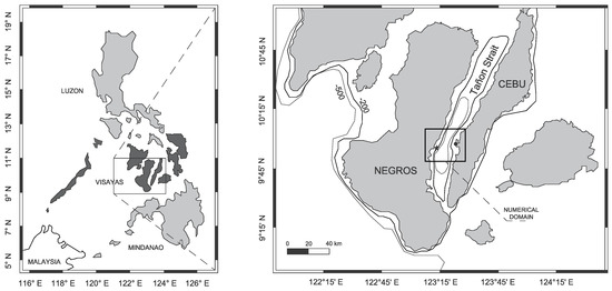
Figure 1.
Map of the Philippines Archipelagos, (left); closer view of Negros and Cebu islands, (right). The black star is located at the epicenter position, while the black dot is approximately at the scuba-diver position during the earthquake. The rectangle indicates the domain reproduced numerically.
The Tañon Strait is the water body that divides the islands of Negros and Cebu, where the earthquake occurred. The strait is about 161 km long, and its width varies from 5 to 27 km. The deepest area of the strait covers the region around the earthquake epicenter and the position of the scuba diver, who recorded the underwater audio; here the maximum water depth is almost uniform around 500 m. A tsunami has been generated by the 6.7 Mw earthquake, inundating the coasts of both islands, luckily without relevant damages.
During this event, an Italian scuba diver, Mr. Riccardo Scultz, was diving near the coast of Cebu island recording with a GoPro camera. His position has been reconstructed to be at N; E, at a water depth of 11 m. He reports to have noticed first a vibration of the sea-floor and suddenly fishes behaving differently; then he heard an anomalous noise. Few minutes later he was out of the water on the boat with the other scuba-divers; they perceived the tsunami waves and they sailed offshore.
Both video and audio records provided by the scuba-diver have been carefully analyzed in [13]. The authors reconstructed the time sequence of the events from the video and audio record, and computed the seismic and hydro-acoustic waves arrival times, using mean pressure wave celerity in ground and in water. The distance epicenter-measurement is 12 km, therefore the approximate seismic and hydro-acoustic waves arrival times are expected after 4 and 8 s respectively from the quake, considering a wave celerity in ground of 3000 m/s and in water of 1500 m/s.
In the previous work, [13] performed a time-series analysis of the audio record, subdividing it in windows of 34 s: one before the computed arrival time of the hydro-acoustic waves, one immediately after and others later. We report in Figure 2 the frequency spectrum of the recorded signal before and after the computed arriving time of acoustic waves. Looking at the frequency spectra of the time series before the earthquake, it can be noted that the amplitude oscillations are in the frequency range of 80–180 Hz, which can be considered the frequency band of the background noise. Considering the time interval immediately after the estimated arrival time of hydro-acoustic wave (lower panel of Figure 2), the acoustic signal oscillates also at lower frequencies, i.e., 10–50 Hz. Since this specific spectral signature recorded after 8 s from the earthquake has not been detected within other time interval of the signals, it is assumed that it is likely to be related the hydro-acoustic waves generated by the sea-bottom displacement. By simulating the generation and propagation of hydro-acoustic waves in the vertical section trough the epicenter and the scuba-diver position, [13] have demonstrated that these pressure waves show a spectral signature similar to that recorded. Therefore, in this paper in order to deeply investigate in the generation and propagation modelling of hydro-acoustic waves, 3D numerical simulation has been carried out.
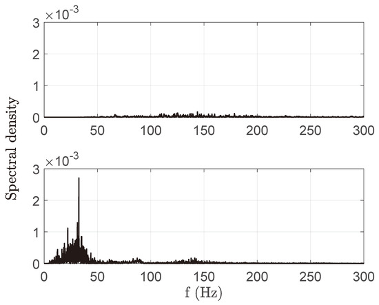
Figure 2.
Frequency spectra of the time series intervals before (upper panel) and immediately after (lower panel) the computed arrival time of the hydro-acoustic waves.
3. Numerical Simulations
Three-dimensional numerical simulations that cover the entire seismic fault zone have been implemented. In the next subsection, details of the model are given, in the following results are presented in term of pressure waves time series at the measuring point, i.e., scuba diver approximate location.
3.1. Description of the Numerical Model
The model solves the wave propagation in weakly compressible inviscid fluid, where waves are generated by a sea-bed motion. In the framework of the linear theory, the governing equation for the fluid potential is:
where is the Laplacian in the horizontal plane , while subscripts with independent variables denotes partial derivatives, is the celerity of sound in water, set as 1500 m/s. The free surface boundary condition that includes both dynamic and kinematic conditions, is set as:
where g is the gravity acceleration. The waves are generated by imposing the following condition at the sea-floor boundary:
where h is the water depth, given by the rest bottom topography net of the earthquake bottom motion
From (4) the water depth time-variation is zero everywhere except on the earthquake zone. In order to reproduce the sea-bed velocity due to the earthquake (), the [15] formula has been used to calculate the sea-floor static deformation from the principal seismic parameters. This deformation has been assumed to occur in the time interval of 1 s. Following the study of [14] the fault zone is characterized by 210° strike, 47° dip; 90° rake and a fault length of 20 km.
The numerical domain in between the free-surface and the sea-floor, is confined by two artificial surfaces at the lateral boundaries, separating the domain from the open sea, where the approximate radiation condition, valid for planar waves orthogonal to the boundary is imposed:
where n indicates the direction normal to the considered boundaries.
In Figure 3 is represented the bathymetry of the Tañon Strait in plan view (left) and in 3D view (right). The available nautical charts of the area have been used to extract the bathymetric data, which have been interpolated over a regular grid, equally spaced in x and y direction each 100 m, and used as bottom surface of the numerical domain.
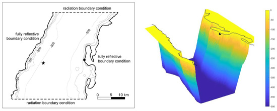
Figure 3.
Reconstruction of the Tañon Strait bathymetry, used in the 3D numerical domain (right plot). In the (left plot) the star indicates the earthquake epicenter, and the dot the measuring position.
A 3D mesh with linear elements has been built, with maximum and minimum element size of 100 m and 0.5 m respectively. A scale geometry has been used to distinguish between horizontal and vertical planes, for x and y directions indeed a mesh up to 10 times larger is used. The mathematical problem is solved using the Finite Element Method, using the Multifrontal Massively Parallel sparse direct Solver (MUMPS). Time integration is carried out for 100 s, with a of 0.005 s.
3.2. Comparison with In-Situ Records
In order to compare the numerical results with the audio recorded, the former have been extracted at the location where approximately the video and audio signals have been measured during the earthquake. Mr. Scultz reported that he was diving approximately at 11 m of water depth; he was not there for scientific purpose and accidentally recorded the video and audio during the earthquake, therefore the water depth during the measurement is assumed to be 11 m, however it is not known precisely. In Figure 4 the comparison is shown. We report the spectral signal recorded (Figure 4a) and those reproduced numerically(Figure 4c), including the results of the two dimensional simulation of [13] (Figure 4b). The three spectra in Figure 4 report the moving average of the original signals, using a frequency window of 2 Hz. Both numerical simulations confirm that hydro-acoustic waves generated by 2012 Negros-Cebu earthquake exhibit a spectral signature very similar to that recorded. Differences in the signals are due to different reasons. Firstly, the recorded signal has been considered for a time interval of 34 s, however was not filtered from the background noise. Then, the coastline reproduced in the numerical models is assumed as fully reflective boundary, i.e., impermeable wall. Moreover, the sea-floor has been considered impermeable, the effect of unconsolidated sediment on the hydro-acoustic wave propagation has been neglected. The uncertain on the exact recording position and water depth, would also affect the quality of the comparison, since as proved by [16] the water depth and the distance from the epicenter significantly influence the pressure field. We remark here that the aim of the simulation was to investigate on the frequency band of the hydro-acoustic wave energy. The comparison of the spectral signals is only qualitative, because carried out without knowledge of the frequency response of the GoPro camera, contained in a impermeable pocket.
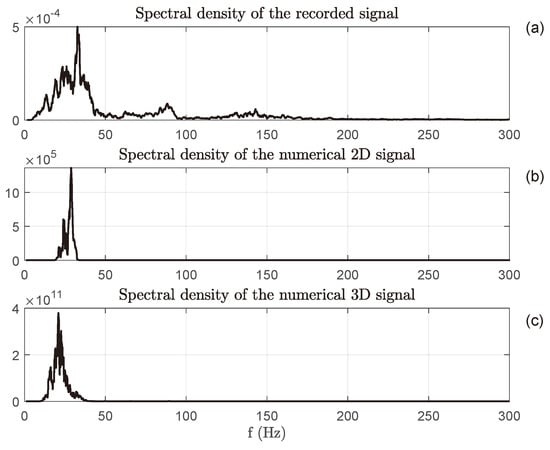
Figure 4.
Spectral signal recorded by the GoPro after the earthquake (a) and spectral signal of the hydro-acoustic waves reproduced numerically by the 2D model of [13] (b) and by the present 3D model (c).
The 3D model result confirms that hydro-acoustic waves propagate within the frequencies range 10–50 Hz. Considering the full 3D bathymetry, a slightly more broad spectrum can be noted, in comparison with the result of 2D simulation. Thus the present results appear to be more similar to the measurements than those obtained using the 2D computations. As stated by [12,16] the water depth and the sea floor morphology affect the hydro-acoustic wave propagation. However for the present case the sea-floor does not present sea mounts or sea-trenches between the epicenter and the recording location, justifying even 2D simulation along the vertical section.
4. Conclusions
The spectral analysis of the underwater audio record, during the Negros-Cebu 2012 earthquake, revealed a specific signature that was attributed by [13] to the measurement of propagated hydro-acoustic waves. This paper completes the previous work, performing 3D numerical simulation over the sea-floor that includes the entire seismic fault. The sea-bed displacement has been reconstructed using the Okada formula [15] and the seismic data elaborated by [14]. The time interval needed to reach the so computed static deformation has been assumed equal to 1 s. A parametric analysis varying the velocity of the sea-bed motion has been carried out in 2D, i.e., considering only the vertical section of the water layer that connect the center of the seismic zone with the position of the recording scuba-diver. The result of the present 3D analysis confirms that hydro-acoustic wave energy is distributed in the frequency range of 10–50 Hz, as stated by [13] and confirmed by the audio record. Given the fault length and the bathymetry uniform along the strike direction of the earthquake, the 3D model provides a slight improvement in the acoustic signal reproduction for this event.
Author Contributions
Data curation, C.C. and A.R.; resources, P.D.G.; software, C.C. and G.B.; writing—original draft preparation, C.C.; writing—review and editing, C.C., A.R., G.B. and P.D.G.
Funding
This research received no external funding.
Acknowledgments
The authors are very grateful to Riccardo Scultz, and his son Giovanni, authors of the underwater video and audio recording, who made them available for this work.
Conflicts of Interest
The authors declare no conflict of interest.
References
- Yamamoto, T. Gravity waves and acoustic waves generated by submarine earthquakes. Int. J. Soil Dyn. Earthq. Eng. 1982, 1, 75–82. [Google Scholar] [CrossRef]
- Nosov, M. Tsunami generation in compressible ocean. Phys. Chem. Earth, Part Hydrol. Ocean. Atmos. 1999, 24, 437–441. [Google Scholar] [CrossRef]
- Stiassnie, M. Tsunamis and acoustic-gravity waves from underwater earthquakes. J. Eng. Math. 2010, 67, 23–32. [Google Scholar] [CrossRef]
- Eyov, E.; Klar, A.; Kadri, U.; Stiassnie, M. Progressive waves in a compressible-ocean with an elastic bottom. Wave Motion 2013, 50, 929–939. [Google Scholar] [CrossRef]
- Maeda, T.; Furumura, T. FDM simulation of seismic waves, ocean acoustic waves, and tsunamis based on tsunami-coupled equations of motion. Pure Appl. Geophys. 2013, 170, 109–127. [Google Scholar] [CrossRef]
- Sammarco, P.; Cecioni, C.; Bellotti, G.; Abdolali, A. Depth-integrated equation for large-scale modelling of low-frequency hydroacoustic waves. J. Fluid Mech. 2013, 722, R6. [Google Scholar] [CrossRef]
- Cecioni, C.; Bellotti, G.; Romano, A.; Abdolali, A.; Sammarco, P. Tsunami early warning system based on real-time measurements of hydro-acoustic waves. Procedia Eng. 2014, 70, 311–320. [Google Scholar] [CrossRef]
- Cecioni, C.; Abdolali, A.; Bellotti, G.; Sammarco, P. Large-scale numerical modeling of hydro-acoustic waves generated by tsunamigenic earthquakes. Nat. Hazards Earth Syst. Sci. 2015, 15, 627–636. [Google Scholar] [CrossRef][Green Version]
- Cecioni, C.; Bellotti, G. On the resonant behavior of a weakly compressible water layer during tsunamigenic earthquakes. Pure Appl. Geophys. 2018, 175, 1355–1361. [Google Scholar] [CrossRef]
- Bolshakova, A.; Inoue, S.; Kolesov, S.; Matsumoto, H.; Nosov, M.; Ohmachi, T. Hydroacoustic effects in the 2003 Tokachi-oki tsunami source. Russ. J. Earth Sci. 2011, 12. [Google Scholar] [CrossRef]
- Abdolali, A.; Cecioni, C.; Bellotti, G.; Sammarco, P. A depth-integrated equation for large scale modeling of tsunami in weakly compressible fluid. Coast. Eng. Proc. 2014, 34. [Google Scholar] [CrossRef][Green Version]
- Abdolali, A.; Cecioni, C.; Bellotti, G.; Kirby, J.T. Hydro-acoustic and tsunami waves generated by the 2012 Haida Gwaii earthquake: Modeling and in situ measurements. J. Geophys. Res. Ocean. 2015, 120, 958–971. [Google Scholar] [CrossRef]
- Cecioni, C.; Romano, A.; Bellotti, G.; De Girolamo, P. Hydroacoustic Waves Measured during the 2012 Negros-Cebu Earthquake. J. Waterw. Port Coast. Ocean. Eng. 2018, 144, 06018004. [Google Scholar] [CrossRef]
- Aurelio, M.; Dianala, J.; Taguibao, K.; Pastoriza, L.; Reyes, K.; Sarande, R.; Lucero, A. Seismotectonics of the 6 February 2012 Mw 6.7 Negros Earthquake, central Philippines. J. Asian Earth Sci. 2017, 142, 93–108. [Google Scholar] [CrossRef]
- Okada, Y. Surface deformation due to shear and tensile faults in a half-space. Bull. Seismol. Soc. Am. 1985, 75, 1135–1154. [Google Scholar]
- Oliveira, T.C.; Kadri, U. Pressure field induced in the water column by acoustic-gravity waves generated from sea bottom motion. J. Geophys. Res. Ocean. 2016, 121, 7795–7803. [Google Scholar] [CrossRef]
© 2019 by the authors. Licensee MDPI, Basel, Switzerland. This article is an open access article distributed under the terms and conditions of the Creative Commons Attribution (CC BY) license (http://creativecommons.org/licenses/by/4.0/).