Permafrost Degradation within Eastern Chukotka CALM Sites in the 21st Century Based on CMIP5 Climate Models

Abstract

Permafrost degradation caused by contemporary climate change significantly affects arctic regions. Active layer thickening combined with the thaw subsidence of ice-rich sediments leads to irreversible transformation of permafrost conditions and activation of exogenous processes, such as active layer detachment, thermokarst and thermal erosion. Climatic and permafrost models combined with a field monitoring dataset enable the provision of predicted estimations of the active layer and permafrost characteristics. In this paper, we present the projections of active layer thickness and thaw subsidence values for two Circumpolar Active Layer Monitoring (CALM) sites of Eastern Chukotka coastal plains. The calculated parameters were used for estimation of permafrost degradation rates in this region for the 21st century under various IPCC climate change scenarios. According to the studies, by the end of the century, the active layer will be 6–13% thicker than current values under the RCP (Representative Concentration Pathway) 2.6 climate scenario and 43–87% under RCP 8.5. This process will be accompanied by thaw subsidence with the rates of 0.4–3.7 cm∙a⁻¹. Summarized surface level lowering will have reached up to 5 times more than current active layer thickness. Total permafrost table lowering by the end of the century will be from 150 to 310 cm; however, it will not lead to non-merging permafrost formation.

1. Introduction

Seasonal soil thaw is the process covering vast areas in cold regions of the Earth [1,2]. Its spatio-temporal variability depends on climatic and landscape parameters [3]. The active layer resulting from this process plays a key role in water, energy and carbon exchange [4,5,6] in local, regional and global scales. Seasonal thaw properties, especially its thickness, define subjacent permafrost conditions and the intensity of the exogenous processes [7,8,9].

Detecting leading natural factors that influence seasonal thaw dynamics in particular regions is urgent for applied studies and fundamental issues [10,11,12], since it allows us to develop prognostic estimations of active layer thickness (ALT) due to climate change [13] and anthropogenic impact [14,15]. Contemporary methods of forecasted ALT calculation enable us to predict its behavior in the future with adequate accuracy at global [16] and regional levels [17,18]. However, such forecasts tend to be inaccurate due to (1) the high local variability of ALT [10], (2) the lack of factual data on heat-exchange conditions on soil surface and within surficial layer [19], and (3) the scarcity of field monitoring network sites in remote areas [20]. Another issue is that climatic models only work well at a global scale [21], which decreases the spatio-temporal resolution of ALT forecasts [22].

This article is the first attempt to estimate ALT and soil surface subsidence prognostic dynamics for the region of Eastern Chukotka, based on accumulated field data on seasonal thawing and selected optimal climate model for this area. We present the projections of seasonal thawing depths and soil surface subsidence for 2 CALM sites, representing the conditions of coastal plains of Eastern Chukotka for the 21st century. The projections are based on simple models of seasonal thawing and data on air temperature and precipitation obtained in the framework of CMIP5 project for “hard” RCP 8.5 (providing for the greatest increase in greenhouse gas content in the atmosphere and the most intense warming) and “soft” RCP2.6 (which preserves the present-day CO2 content in the atmosphere) climate scenarios.

2. Study Area

2.1. Natural Conditions of Eastern Chukotka

The coastal plains of Eastern Chukotka are gently sloping foothills, adjacent to the flattened low-hill terrain, which is composed of Mesozoic folded rocks. They make up approximately 20% of the region area [23] and occupy the Mechigmen-Kolyuchin depression in its western and southern parts, as well as narrow (up to 50 km) coastal stripes in the north and east. These surfaces are represented by the Middle Pleistocene marine plains, the Holocene marine spits, river valleys, and the fluvioglacial and moraine plains of Pleistocene age, dotted with bogs and thermokarst lakes [24,25].

Eastern Chukotka is located in arctic and subarctic climate zones and is significantly influenced by marine air masses. Summer is cloudy and cool: T_jul +8 + 10 °C. Winter is long, with frequent and prolonged blizzards, T_jan −16–20 °C. The average annual rainfall grows from north to south from 230 (Uelen) to 690 mm (Provideniya); mean air annual temperature (MAAT) vary from −6.9 °C to −4.0 °C respectively This is a polar tundra zone according to Köppen-Geiger Climate Classification [26,27,28].

The study area is characterized by continuous permafrost distribution. Taliks are only present under large rivers and lakes. Permafrost thickness within coastal plains is 100–200 m [24,29]. Mean annual ground temperature (MAGT) in the study area varies from −4 to −6 °C [29]; however, the results of direct thermal observations in this area are not available. Thermokarst and thermoerosion forms are widespread [24]. Permafrost in this region is presented by mostly epigenetic rocks with low ice content (up to 15%). Syngenetic sediments are less spread and presented mostly by alluvium, slope and biogenic deposits developed from the surface and reaching ice content of 50–60% [30].

Due to the cooling and moisturizing effect of the sea, barrens and cryptograms are common on the tops and slopes of the hills at altitudes higher 50 m above sea level. Smooth slopes and low interfluves are covered with low-shrub and tussock tundra with a predominance of Ereophorum vaginatum and Carex lugens. The depressions between the hummocks are occupied by swampy hollows of Sphagnum. Intense shrub-grass, sedge and moss vegetation is characteristic of river valleys, marine terraces and deep hollows of the lower part of the mountains.

2.2. Active Layer Monitoring Sites

There are two sites for measuring the active layer on the plains of Eastern R27 Chukotka: Lavrentiya and R41 Lorino (Figure 1 and Figure 2). They both are part of the program for Circumpolar Monitoring by the Active Layer (CALM) program [31,32]. In terms of landscape, both sites represent Tussock-sedge, dwarf-shrub, moss tundra (G4) and Sedge, moss, dwarf-shrub wetland (W2), covering almost 25% of the Eastern Chukotka coastal plains area (

Table 1. Vegetation units of Eastern Chukotka coastal plains and their representation for the Arctic region [33].

Vegetation Unit	Area, sq. km	Area, %	Total % of the Arctic Area 1
Non-carbonate mountain complex (B3)	17,803.2	33.4	10.7
Non-tussock sedge, dwarf-shrub, moss tundra (G3)	874.7	1.6	11.3
Tussock-sedge, dwarf-shrub, moss tundra (G4)	8767.8	16.5	6.7
Erect dwarf-shrub tundra (S1)	5206.4	9.8	13.7
Low-shrub tundra (S2)	17,368.0	32.6	12.7
Sedge, moss, dwarf-shrub wetland (W2)	3248.6	6.1	2.7
Total	53,268.7	100.0	57.8

¹ Excluding glaciers.

) [33].

Lavrentiya monitoring site (65°36′ N, 171°03′ W; CALM R27) was founded in 2000. It is located 3 km NW of the settlement Lavrentiya, 0.8 km from the coast of Saint Lawrence Bay, between a barren ridge and a flat marine terrace. The surface has a prominent micro-relief and soft slope (2–3°) to the NE; its absolute height is about 70 m. The deposits are glacial boulder loams covered with a thin peaty layer. The main part of the site is represented by wet sedge-willow tundra on Gleyic-Histic Cryosols; shrub-grass associations grow on the bumps.

ALT measurements at the Lorino site (65°32′ N, 171°38′ W; CALM R41) have been carried out since 2010. It is located about 4 km NE of the Lorino settlement, on a flat wetland. The site surface has is hilly and swampy and located at an altitude of 40–42 m above sea level. The active layer is represented by peat throughout almost the whole site. According to marine coastal outcrops, 2 km from the site, the surficial peat horizon is underlain by boulder loams. The vegetation is more diverse than at Lavrentiya site: sedge and lichen-shrub communities are present on the bumps, whereas sedge-sphagnum communities occupy the depressions.

3. Materials and Methods

3.1. Field Data

Field measurements of ALT at monitoring sites have been being conducted according to standard protocol [31] since 2000. Every site represents 100 × 100 m grid with measurement nodes, located 10 m from each other—121 nodes in total. Thaw depth in every grid node is average value of 4 measurements around it. ALT is defined by penetrating the thawed ground with a steel rod until permafrost table with an accuracy of 1 cm. The measurements are conducted several times in a season throughout July, August, and September. The maximal thaw depths are reached in late September, when daily average temperature drops below 0 °C. If field measurements were not conducted in that period, the maximal ALT is re-calculated using the last measured values and strong linear correspondence of ALT and square root of accumulated thaw degree days (I_t) [35].

Surficial (0–7 cm) layer soil moisture and thaw settlement are measured simultaneously in equal proportions with ALT. The moisture content is obtained by Vital Hydra logger and Thetha probe HH2 Moisture Meter through calculating electrical permittivity. Soil thaw subsidence is obtained by measuring the height of the iron stakes, which are set into the upper layers of permafrost in every node of Lavrentiya CALM site. The measurements were taken twice for every stake by single person (A. Maslakov) with single millimeter accuracy yardstick, which was pressed on soil surface with the same force. The stakes heights determination in the end of thaw season allows defining summer subsidence, while measurements in its beginning allow revealing approximate winter frost heave values. Surface movement dynamics data are available for the Lavrentiya site only.

At the CALM sites temperature of active layer has been monitored since 2012; however, continuous temperature measurements were initiated in 2014 only. Sensors are installed at a depth from 0 to 100 cm and plugged to Hobo data loggers, which register temperature every hour. Besides, data from the 21X data logger, which was set next to the Lavrentiya site and registered both air and soil surface temperatures every half an hour during 2015–2018, was used in this study.

Data on thermal conductivity were obtained from soil investigation report for local road from Lavrentiya to Lorino settlements and from our sampling in summer 2018. The data on moisture distribution within the active layer were taken from H21-USB data-logger.

3.2. Climate Data

To determine the ALT and soil subsidence, data on air temperature and precipitation are required (active layer models are presented below). Based on various data sets (observations, reanalysis, CMIP5 models), the annual sums of positive and negative daily average temperatures are calculated. They are degree days of thawing and freezing I_t (DDT)) and I_f (DDF), and the sum of precipitation in the warm and cold period.

3.2.1. Observation and Reanalysis Data

The ALT monitoring sites are located in a remote region of the Chukotka Peninsula, which is not covered by hydrometeorological network observations. The nearest weather stations Uelen (66°10′ N, 169°50′ W; WMO ID:25399) and Provideniya (64°25′ N, 173°15′ W; WMO ID:25594) are 87 and 145 km away, respectively (Figure 3) [28]. Therefore, to describe the hydrometeorological conditions at the CALM sites, NCEP/NCAR reanalysis data [36] were used in proximate grid node to the CALM sites land. The reanalysis grid step is 2.5°. The quality of climatic parameters reproduction in this region is not too high: the root mean square deviations (RMSD) of observation series at Uelen and Provideniya stations from the data from the nearest reanalysis land grid node is 6–9% for the freezing index and about 10% for the thawing index, whereas the correlation coefficients are 0.80–0.90 and 0.66–0.88, respectively.

3.2.2. CMIP5 Project Data

Climate parameters were projected from 14 climate models of the 5th phase of the Coupled Model Intercomparison Project (CMIP5, [37]). The list of the models used is presented in

Table 2. The list of used climate models CMIP5 and its major parameters.

	Model	Horizontal Grid Resolution (Degrees) 1		Country	Institution
		at Latitude	at Longitude
1	CNRM-CM5	1.40625	1.40625	France	Centre National de Recherches Meteorologiques/Centre Europeen de Recherche et Formation Avancees en Calcul Scientifique
2	CSIRO-Mk3-6-0	1.875	1.875	Australia	Commonwealth Scientific and Industrial Research Organisation in collaboration with the Queensland Climate Change Centre of Excellence
3	NOAA GFDL-CM3	2	2.5	USA	Geophysical Fluid Dynamics Laboratory
4	GFDL-ESM2G	2	2.5
5	GFDL-ESM2M	2	2.5
6	IPSL-CM5A-LR	1.875	3.75	France	Institut Pierre-Simon Laplace
7	IPSL-CM5A-MR	1.25874	2.5
8	MIROC-ESM	2.8125	2.8125	Japan	Atmosphere and Ocean Research Institute (The University of Tokyo), National Institute for Environmental Studies, and Japan Agency for Marine-Earth Science and Technology
9	MIROC-ESM-CHEM	2.8125	2.8125
10	MIROC5	1.40625	1.40625
11	MPI-ESM-LR	1.875	1.875	Germany	Max Planck Institute for Meteorology (MPI-M)
12	MPI-ESM-MR	1.875	1.875
13	MRI-CGCM3	1.125	1.125	Japan	Meteorological Research Institute
14	NorESM1-M	1.89474	2.5	Norway	Norwegian Climate Centre

¹ The grids of some models have variable pitch. The specified value is close to the average.

. Only models that represent data for the entire period 1900–2100 were selected for both parameters (air temperature and precipitation) and for both climate scenarios. Among the two climatic scenarios, one was considered as “hard” RCP8.5, which implies the greatest emissions of greenhouse gases into the atmosphere and the greatest intensity of warming, and the other as “soft” RCP2.6, which preserves concentrations at the level of 2020–2030.

The climate models’ data include two sets of arrays: the historical part describes the climate in 1901–2010, the forecasting part in 2011–2100. The models have resolutions from 1.125° to 2.8125°. The data on temperature and precipitation were linearly interpolated into a grid with a resolution of 0.5°. The ensemble average is calculated for each day and then the values were accumulated to get seasonal sums for each model and for the ensemble mean. To evaluate the measure of uncertainty the models’ values distribution was analyzed for each year: the 14 values were ranged and the two top and two bottom values were excluded. The 3rd and the 12th values in the range describe the upper and lower estimates. In total, 71.4% of models (10 of 14) reproduce the values within the derived bound. To get off the high-frequency noise, the 11-year running mean filter was used for upper and lower estimates.

The historical part of the models and their ensemble are compared with the observations data and reanalysis of NCEP/NCAR for the periods whereas the data from all the sources are available (observations at both stations, reanalysis, models): thawing indexes for 51 years: 1948–1976, 1978–1993, 1998–2001, 2003–2004; and freezing indexes for 50 years: 1949–1976, 1978–1993, 1998–2001, 2004–2005.

The IPCC reports [21] emphasize that climate models satisfactorily reproduce climate on a global scale and much worse on a regional scale. Moreover, it is difficult to expect high reliability of climate projections on the scale of the model grid cell. Indeed, the comparison of climate model and reanalysis data showed significant differences: for various models the standard deviation of CMIP5 series, corrected for systematic deviation, for freezing index is 350–750 °C-days (15–25% of long-term average annual value,

Table 3. Root mean square deviations (RMSD) of CMIP5 models datasets and their ensemble from the data of reanalysis NCEP/NCAR for accumulated temperature (DDT and DDF, °C-days) and precipitation amount in warm and cold periods (cm) in fractions from long-term average annual value (1948–2010). The nearest grid cell to the CALM site 0.5 × 0.5° and averaged value for the region 63–70° N and 165° E–168° W were considered.

	Model	Temperature				Precipitation Amount
		DDF		DDT		Cold		Warm
		Cell	Region	Cell	Region	Cell	Region	Cell	Region
1	CNRM-CM5	0.18	0.12	0.23	0.20	0.41	0.27	0.45	0.25
2	CSIRO-Mk3-6-0	0.25	0.12	0.22	0.16	0.36	0.26	0.51	0.23
3	GFDL-CM3	0.20	0.09	0.27	0.22	0.33	0.24	0.45	0.23
4	GFDL-ESM2G	0.17	0.09	0.21	0.16	0.28	0.24	0.35	0.24
5	GFDL-ESM2M	0.18	0.10	0.25	0.18	0.34	0.25	0.38	0.24
6	IPSL-CM5A-LR	0.16	0.09	0.29	0.20	0.34	0.27	0.50	0.26
7	IPSL-CM5A-MR	0.18	0.11	0.24	0.24	0.38	0.31	0.58	0.26
8	MIROC-ESM	0.17	0.10	0.29	0.20	0.37	0.26	0.47	0.31
9	MIROC-ESM-CHEM	0.15	0.10	0.31	0.19	0.36	0.29	0.56	0.25
10	MIROC5	0.19	0.10	0.26	0.22	0.35	0.26	0.43	0.28
11	MPI-ESM-LR	0.17	0.11	0.27	0.27	0.28	0.28	0.45	0.24
12	MPI-ESM-MR	0.18	0.10	0.24	0.22	0.36	0.28	0.48	0.28
13	MRI-CGCM3	0.17	0.12	0.23	0.16	0.37	0.29	0.46	0.29
14	NorESM1-M	0.20	0.11	0.25	0.20	0.28	0.26	0.37	0.24
	Ensemble	0.12	0.07	0.20	0.14	0.25	0.22	0.33	0.20

); for the thawing index is 100–200 °C-days (21–31%). For the ensemble of models, the deviation is 12 and 20% for the freezing and thawing index respectively.

Assuming that the reliability of the projections increases with a decrease of study scale, in this paper climate projections are made not only for the local cell of the model grid, but also for the Chukotka region (63–70° N and 168–179° W) and the Northeastern tip of Siberia: 63–70° N and 165° E–168° W (see Figure 3). The climatic parameters were averaged within these regions according to reanalysis data and climatic models (only grid cells occupied by land were taken for averaging). It was certainly the case that the climate model estimates get better with the averaging region expansion. For thermal characteristics on regional scale, climate model estimates (RMSD) were for Chukotka region 3–4% and for the Northeastern tip of Siberia 5–6% better than on the grid cell scale. For the big region, the standard deviation of the models’ ensemble for the freezing index was 7%, for the thawing index −14% (Table 3). For precipitation, the gain in the quality estimates as 3 and 7% for the cold and warm periods, respectively: the RMSD of the ensemble of models is 22 and 20%. In order to obtain a projection of climatic parameters for 21st century in the area of the CALM sites, the average values for the Chukotka region were adjusted for the deviation of long-term average annual values closest to the sites from the regional average in the grid node.

3.3. Seasonal Thaw Models

Based on the ensemble average values of climatic parameters, projections of ALT were obtained using three models: linear regression method, Stefan and Kudryavtsev equations. The resulting series were smoothed by an 11-year moving averages.

Regarding model ensemble, we use the climatic parameters ensemble mean values to calculate the most probable ALT value. The climatic parameters upper and lower estimates (see Section 3.2.2) are used to describe the ALT uncertainty for each seasonal thaw model (regression, Kudryavtsev and Stefan). The derived three uncertainty bounds were combined using the highest and the lowest ALT-estimates values. The resulting uncertainty bound describes about 71.5% of presumable projections, as do the incoming climatic parameters. The described procedure was applied for CPIM5 historical part and both projections.

3.3.1. Regression Model

Regression analysis is the method the research of measured parameters modeling and their properties [38]. Such a model is empirical and reflects the actual interrelation of various independent quantities with the dependent parameter. The accuracy of the model depends on the quality and quantity of input parameters. The regression models of seasonal thawing have an advantage over the other ones in that they are more flexible for describing the process of seasonal thawing at a specific point, and take into account the interrelations of natural features that are characteristic only for a particular local area or site.

3.3.2. The Stefan Model

The Stefan solution to the heat-transfer problem in a solid medium with phase change provides a useful analytical method for predicting active layer thickness [39]. This is one of the simplest and most popular models for calculation of seasonal freezing/thawing depth [40,41]. The Stefan model can be expressed in its simplest way as Equation (1):

$$z=\sqrt{\frac{2K_{t}s{I}_t}{\rho L}},$$

(1)

where z is active layer thickness (m), K_t is thermal conductivity of thawed soil (W∙m⁻¹∙°C⁻¹), s is a scaling factor (86 400 s∙d⁻¹), I_t is the air temperature thawing/freezing degree days sum (°C∙d), ρ is soil density (kg∙m⁻³), and L is the latent heat of fusion (J∙kg⁻¹).

Stefan model is often used in a modified form [35,42]:

$$z=E\sqrt{I_t},$$

(2)

where E is an edaphic, or pedologic factor, defining conditions of heat transfer on the surface and in thawing soil. It is independent on temporal variations of climatic characteristics (e.g., air temperature).

Edaphic factor can be calculated in Equation (3):

$$E=\sqrt{\frac{2K_{t}ns}{\rho L}},$$

(3)

where n is the dimensionless ratio of seasonal ground-surface and degree-day sums of air temperature, known as an n-factor. Edaphic factor can be also calculated from (2) in the case of long-term observations of seasonal thaw depth.

Thus, the only dataset of measured ALT and predicted I_t are required for this model implementation.

3.3.3. Kudryavtsev Model

Kudryavtsev equation [43] and its further modification [44,45] is an alternative solution to the Stefan problem. Although it requires much more input data on the thermophysical properties of the active layer column, its surface and base, this is the most precise model for seasonal thaw calculation.

Initially, the Kudryavtsev equation is expressed as Equations (4)–(6):

$$z=\frac{2\left(A_{gs}-\left|\overline{T_{ps}}\right|\right)\sqrt{\frac{K_t{C}_{t}P}{\pi }}+\frac{(2\overline{A}{C}_t{X}_{2C}+\rho Lz)\rho L\sqrt{\frac{K_{t}P}{C_t\pi }}}{2\overline{A}{C}_t{X}_{2C}+\rho Lz+(2\overline{A}{C}_t+\rho L)\sqrt{\frac{K_{t}P}{C_t\pi }}}}{(2\overline{A}{C}_t+\rho L)},$$

(4)

With

$$\overline{A}=\frac{A_{gs}-\left|\overline{T_{ps}}\right|}{ln\frac{A_{gs}+\frac{\rho L}{2C_t}}{\left|\overline{T_{ps}}\right|+\frac{\rho L}{2C_t}}}-\frac{\rho L}{2C_t},$$

(5)

$$X_{2C}=\frac{2\left(A_{gs}-\left|\overline{T_{ps}}\right|\right)\sqrt{\frac{K_t{C}_{t}P}{\pi }}}{2\overline{A}{C}_t+\rho L}$$

(6)

where C_t is the thawed volumetric heat capacity (J∙m⁻³∙°C⁻¹), P is the period (one year), A_gs is the amplitude of annual periodic temperature variations at the ground surface (°C), and T_ps is the mean annual permafrost surface temperature (MAPST; °C).

3.4. Thaw Subsidence Model

The seasonal thawing of ice rich sediment where the volumetric ice content exceeds the natural porosity of the soil leads to surface subsidence [9,46,47]. Contemporary thaw subsidence was traced on the CALM sites of European Russia [48] and Alaska [49].

Although thaw subsidence can be calculated with physical models [50], we used an empirical approach since regular field observations of surface changes at Lavrentiya site in 2012–2018 allowed us to establish some patterns of subsidence and heaving processes. With thaw depths lower or close to average values, the degree of summer soil surface lowering is fully compensated by winter frost heaving. In the years of high ALT, when the so-called “transient layer” [51] and the upper horizons of permafrost thaw, the heaving intensity is not enough to compensate for the lowering of the soil surface, since a part of the melted ice is moved away by lateral streams. To assess the predicted changes in surface level at the CALM sites, the following empirical model was developed:

$$s_i={\displaystyle {\sum }_1^n}{z}_i{t}_i-z_{i-1}{f}_i,$$

(7)

where s_i is surface level change in i year, cm. z is thaw depth, cm, t is specific thaw subsidence of soil layer, m·m⁻¹, n is the number of layers in active layer column, f is specific frost heave in winter prior to thaw season, m·m⁻¹. Thus, the total value of soil subsidence for a certain period will be:

$$S={\displaystyle {\sum }_1^i}{s}_i,$$

(8)

Based on the data obtained from Lavrentiya CALM site (see Section 4.1), the differential subsidence model was accepted. The deeper soil thaws are, the greater the subsidence amount is and the less heaving can compensate for the lowering of soil surface (

Table 4. Parameters used for predicted thaw subsidence calculations.

Lavrentiya			Lorino
Layer	Seasonal Thaw Depth, cm	Specific Thaw Subsidence, m·m−1	Layer	Seasonal Thaw Depth, cm	Specific Thaw Subsidence, m·m−1
1	0–60	0.04	1	0–50	0.04
2	60–70	0.06	2	50–60	0.06
3	>70	0.10	3	>60	0.10

). Heave value for the entire column of thawed deposits was taken at 0.04 m·m⁻¹. The depth values were determined by an expert assessment, based on the long-term averages of soil thawing depths at each of CALM sites, so the prediction of subsidence is purely indicative.

The model was used for both sites (Lavrentiya and Lorino) for RCP8.5 and RCP2.6 climatic scenario using 6 (3 for each scenario) modeled ALT values and ALT upper and lower estimates which are calculated as described in Section 3.3.

4. Results

4.1. Weather Characteristics, ALT and Thaw Subsidence Contemporary Variations

As mentioned above, monitoring of seasonal thawing depth in the Eastern Chukotka region was initiated in 2000. During this period (18 years), the weather dataset from the closest weather station (Uelen) was analyzed taking into account the evolution of weather parameters since 1977 (when data are available) to detect the main tendencies and extremes and weigh the rates of future projections. The main parameters that determine the seasonal thawing process were considered: the thawing index (I_t), the freezing index (I_f), winter and summer precipitation amounts (Figure 4). Since 2000 the thawing index varies between 450–950 °C-days with the mean value of 700 °C-days, while in 1977–1999 it was about 615 °C-days. The I_f varies between −3500 and −2000 °C-days with the mean about −2800 °C-days. The previous period is 500 °C-days colder. The detected growth is the result of warming in Chukotka at the end of 20th century. From the 1970s and until 2005, the Uelen weather station recorded an increase in average annual air temperature at a rate of 0.5 °C·decade⁻¹ (p-value 0.004). The same situation was registered at Anadyr weather station (600 km to the south-west of Uelen): for 1980–2010 warming rate was 0.4 °C·decade⁻¹ (p-value 0.08) [28,52]. Precipitation amount indeed does not show any trends: it evolves around 115 mm both in cold and warm season.

The average ALT at Lavrentiya CALM site is 66 ± 5 cm (2000–2017), and at Lorino is 52 ± 4 cm (2010–2017). Despite the absence of trends in weather parameters, the variations of seasonal thawing depths show a weak tendency to increase: the active layer thickening rate for Lavrentiya is 0.5 cm· a⁻¹ (R² = 0.33, n = 18), and for Lorino −1.5 cm a⁻¹ (R² = 0.75, n = 8). Both trends are statistically significant (p-values are 0.01 and 0.005 respectively). However, common trend for most of CALM sites in NE Russia (Kolyma and Anadyr lowlands) identifies the stabilization of seasonal thaw deepening in recent years. This upward trend is characteristic of the air temperature at the end of the 20th and the beginning of the 21st centuries [52,53].

Average summer volumetric moisture content of surficial soil layer was 43–77% for Lavrentiya (median 66%) and 23–83% for Lorino (median 44%).

Regular observations of soil surface level relative to the steel stakes hammered into the permafrost at the Lavrentiya site enabled the tracing of soil surface movement rates (Figure 5). Stakes heights determination in the middle (July) and the end (September) of thaw periods provided measured thaw subsidence values (red solid line), while the difference between stakes heights in July and September of the previous year gives summarized values of frost heave (blue dotted line) and thaw subsidence for the beginning of thaw period (red dotted line). For the period 2012–2018, the rate of soil subsidence was 0.019–0.067 cm·m⁻¹ (average 0.041 cm·m⁻¹). Depending on the season, the values were up to 13.9 cm·m⁻¹ while the average thawing depth on the site reached 70 cm. At the same time, the amount of frost heave is 0.008–0.040 cm·m⁻¹ (average 0.023 cm·m⁻¹). The correlation between thaw depth and subsidence value is significant (r = 0.75, n = 60 to 121 depending on year): the deeper the soil thaws are, the higher the subsidence value is. The frost heaving of the soil could not compensate for the value of thaw subsidence during these years; therefore, the rate of the soil surface lowering was 1.5–2.7 cm·a⁻¹ (average 2.1 cm·a⁻¹), and the total amount of subsidence was 14.6 cm for 7 seasons. Thus, for the period 2012–2018 the lowering of permafrost table for Lavrentiya was 2.6 cm·a⁻¹ due to ALT increase and surface lowering.

4.2. Active Layer Modeling

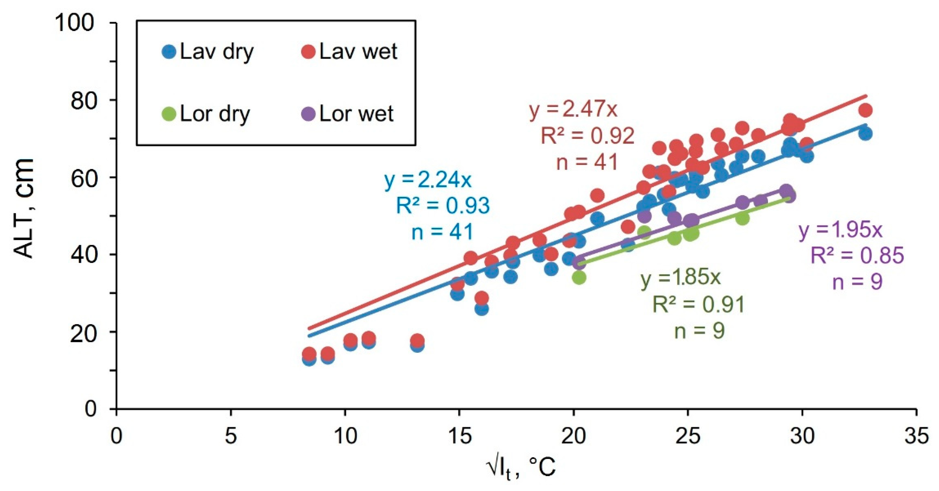
4.2.1. Regression Model

The main natural factor determining short-period variations of seasonal thawing depth is climate [54]. Based on meteorological parameters and measurements of ALT at CALM sites, a multiple regression analysis was performed and linear regression equations were constructed, in which the dependent variable was the maximum seasonal thaw depth for the year (

Table 5. Regression equations for CALM sites in Eastern Chukotka.

Site	Equation Coefficients				Remainder	Approximation Coefficient (R2)
	√It	Summer Precipitation	Winter Precipitation	√If
Lavrentiya	0.79	0.08	−0.06	−0.49	69.2	0.67
Lavrentiya dry	1.18	0.08	−0.05	−0.13	34.9	0.59
Lavrentiya wet	0.82	0.07	−0.04	−0.31	60.8	0.59
Lorino	1.45	0.13	−0.03	−0.28	16.2	0.99
Lorino dry	1.68	0.12	−0.02	−0.29	9.1	0.89
Lorino wet	1.27	0.14	−0.04	−0.27	21.4	0.97

).

As can be seen from Table 5, the main contribution (71–76%) to the inter-annual variations of seasonal thaw depths is made by the thermal factor—the sum of positive (I_t) and negative (I_f) degree-days, while the amount of summer and winter precipitation is in second place (24–29%) that looks quite natural. On average, at the Lavrentiya CALM site, these meteorological characteristics account for 67% of the inter-annual ALT variation, and for Lorino—99%. Such a difference is most likely due to the location of Lorino on a relatively horizontal site in the autochthonous landscape, whereas Lavrentiya is located on a slope and therefore is influenced by neighboring territories (primarily due to horizontal water transfer in the active layer).

Using the results of monitoring the near-surface humidity (0–7 cm) of the soil layer allowed us to identify wetter and drier areas within the sites and also constructing regression equations for them (see Table 5). Dry areas with soil moisture below the median value are characterized by smaller ALT on 2–6 cm than wet ones. At the same time, they show a greater importance of the thawing index compared to wet ones.

4.2.2. Stefan Model

The empirical edaphic factor E for the CALM sites of Eastern Chukotka was obtained by comparing measured seasonal thaw depths and accumulated positive degrees-days (I_t) at the time of field ALT measurements. The resulting relationship is shown in Figure 6.

For the Lavrentiya and Lorino sites, the E coefficient varies between 2.24–2.47 and 1.85–1.95, respectively, depending on soil moisture. The mean values of E were 2.36 (for Lavrentiya) and 1.9 (for Lorino). For the Lavrentiya site, this parameter has already been defined in previous studies [55]. The current value of E has grown compared with the previous one, covering the period 2000–2003, by less than 1%. This allows us to confirm the conclusions about its stationarity and independence from climatic characteristics [56].

4.2.3. Kudryavtsev Model

Compared to other models, the Kudryavtsev equation requires a large number of input characteristics. Obtaining the parameters indicated in Equations (4)–(6) turned out to be difficult and required the introduction of a number of assumptions:

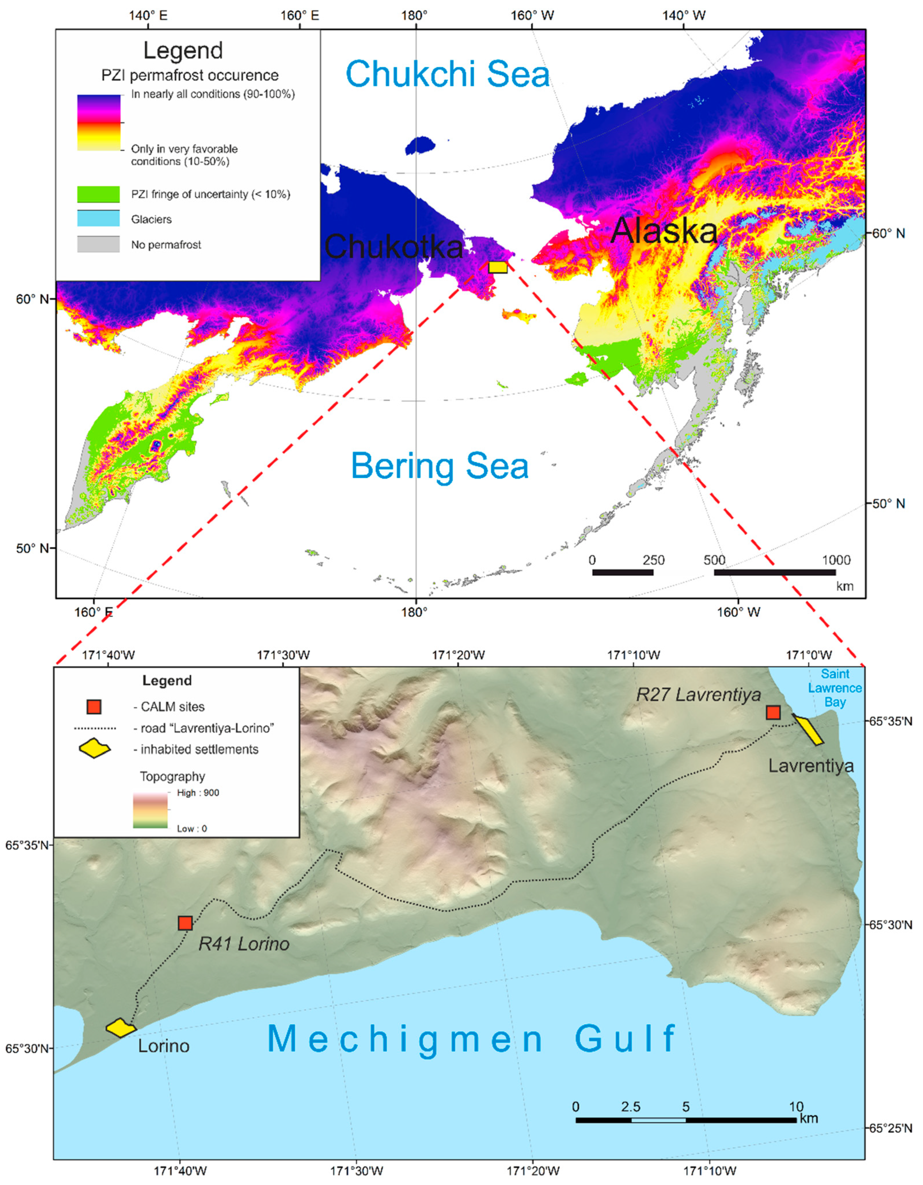
• Soil characteristics of ALT for the Lorino site were used from an engineering survey report along the Lavrentiya-Lorino road, which is 50–300 m from both CALM sites (See Figure 2). Surveys were conducted in 2012 by the company Irkutskgiprodornii, and the report was kindly provided by the administration of the Chukotka administrative district. In order to estimate interannual variability of soil moisture, we compared the results of surficial soil moisture measurements within Lorino CALM site for 2011–2017. Averaged value was 52.2 ± 4.9% with 12.9% spread that was estimated as relatively stable parameter in time. Thus, we considered it possible to use data from engineering surveys in 2012. The required soil parameters are presented in

  Table 6. Thermal properties of the active layer used in the calculations with Equations (4)–(6).

  Site	Average Volumetric Water Content Θ, %	Average Latent Heat ρL, MJ∙m−3	Average Thermal Conductivity Kt, W∙m−1∙°C−1	Heat Capacity Ct, MJ∙m−3∙°C−1
  Lavrentiya	0.27	117.6	0.69	2.63
  Lorino	0.40	140.7	0.51	3.40

  .
• Mean annual permafrost surface temperature (T_ps) for both sites was retrieved from the data logger readings installed on the CALM Lavrentiya site for the period 2014–2017.
• Amplitude of annual periodic temperature variations at the ground surface (A_gs) is the average difference over several years in maximum and minimum mean monthly temperatures of the soil surface [43]. For our calculations it was defined as the difference between mean annual ground surface temperature (MAGST) and the average temperature of the soil surface in the warmest month (usually July or August).
• MAGST was also determined from data loggers at the Lavrentiya site.
• To calculate the thawing depth in the years when temperature observations were not carried out, the average temperature of the soil surface in the warmest month of the year was calculated taking into account the average monthly air temperature. According to data loggers measurements, these characteristics turned out to be approximately equal at this time of year.
• MAPST values were assumed as constant for the entire observation period.

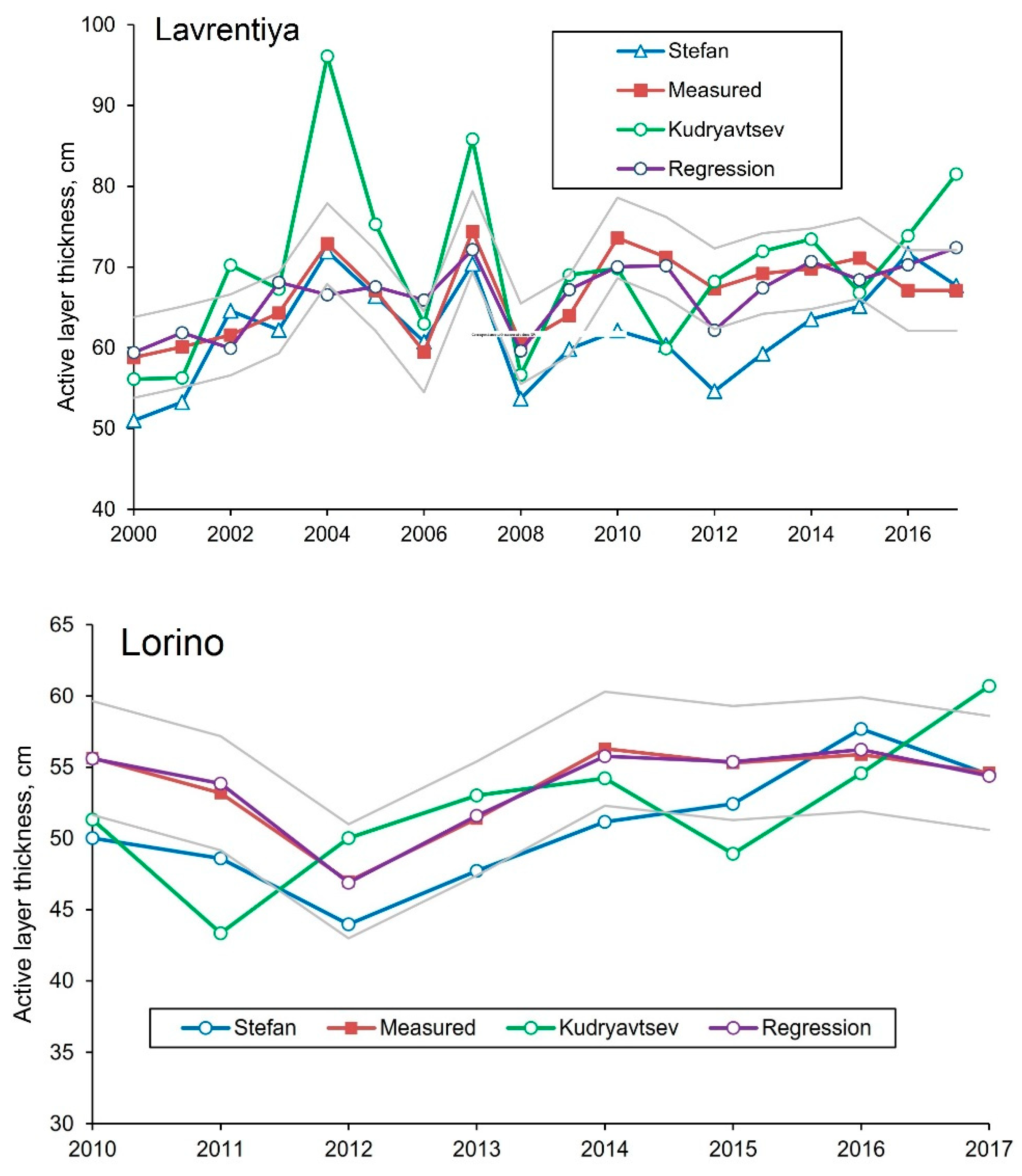
4.2.4. Comparison of Measured and Modeled ALT Data

Comparison of seasonal thaw depths obtained pursuant to the regression model. Stefan and Kudryavtsev equations with measured values (

Table 7. Correspondence of modeled and measured active layer thickness (ALT) data on the CALM sites of Eastern Chukotka.

Model	Lavrentiya			Lorino
	Correspondence with Measured Values (R2)	p-Value	Maximal Difference, %	Correspondence with Measured Values (R2)	p-Value	Maximal Difference, %
Regression	0.67	<0.001	−9 + 11	0.99	<0.001	−1 + 1
Stefan	0.45	0.006	−19 + 7	0.64	0.017	−0 + 3
Kudryavtsev	0.43	0.004	−16 + 32	0.36	0.116	+7–−17

, Figure 7) made it possible to assess the degree of their reliability for Eastern Chukotka CALM sites. The best fit to the measured data is shown by the regression equations with approximation coefficients R² (0.67–0.99) at p-value below 0.001. The Stefan model in a modified form (3) also agrees well with the results of field observations. However, it provides slightly underestimated (by an average of 5–7%) values. The lowest level of compliance with the measured values is shown by the Kudryavtsev equation (see Table 7). The differences are particularly strong for the Lavrentiya site in the warm years of 2004 and 2007, where the model gives the values overestimated by 32 and 15%, respectively. For the Lorino site, due to the relatively short observation period and the low degree of correlation between measured and calculated ALT values, the significance level exceeds the critical value (p > 0.05), and Kudryavtsev model in this case does not statistically correspond to the real seasonal thawing dynamics. This low accuracy is due to the quality of the data entered into the equation and the number of the introduced assumptions (see Section 4.2.3.).

Thus, despite the different levels of confidence, all the models presented to some extent reflect the dynamics of the seasonal thawing process and, when replacing the actual values with the predicted ones, can be used to assess changes in the thickness of the seasonal layer during the 21st century.

4.3. Predicted Climate Change for Eastern Chukotka Region

The projections of climatic characteristics are made according to CMIP5 data for two scenarios: “hard” RCP8.5, which implies the greatest carbon dioxide emissions into the atmosphere and the most intense warming, and “soft” RCP2.6, which preserves the present CO₂ content in the atmosphere. The ensemble of climate models shows that in the case of the RCP 8.5 scenario, the thermal conditions in Chukotka (in terms of thawing and freezing indices) will be close to the current conditions in the Kuril Islands: the freezing index will increase by 2500 °C-days or 75%, reaching values around −700 ° C-days (from 0 to −1500 °C-days for different models), and the thawing index—for 1000 °C-days or 130% to 1750 °C-days (from 1200 to 2500 °C-days for different models). In the case of the RCP 2.6, the warming in the Chukotka region will continue until 2030–2050, with the thawing and freezing indices reaching the values characteristic of Kamchatka (about 1000 and −2000 °C-days, respectively, that is, they will increase by 50% compared to the level of 1960–1990 for both parameters). Such an increase in temperature will inevitably affect the state of permafrost.

It is important to mention that modeled data has significant level of uncertainty. The historical part is simulated with 400 °C-days spread for I_f, 200 °C-days for I_t, 70 mm for winter precipitation, and 50 cm for summer one. Prognostic spread is much higher: 1000 °C-days for both thermal indices and 200 mm for precipitations.

4.4. ALT Dynamics Estimation for 21st Century

The prediction of ALT, performed on the three considered models, considered two climate scenarios (

Table 8. Predicted seasonal thaw depths (cm) for the CALM sites of Eastern Chukotka and its changes in relation to the current values.

CALM Site		Lavrentiya			Lorino
Model		Reg	Ste	Kud	Reg	Ste	Kud
Observed ALT		66.5			52.4
2025–2035	RCP 2.6	69.3 (+4%)	70.9 (+7%)	78.5 (+18%)	59.0 (+13%)	57.1 (+9%)	58.2 (+11%)
	RCP 8.5	70.7 (+6%)	72.5 (+9%)	80.4 (+21%)	60.7 (+17%)	58.4 (+11%)	59.5 (+14%)
2045–2055	RCP 2.6	71.7 (+8%)	72.6 (+9%)	79.7 (+20%)	62.0 (+18%)	58.5 (+12%)	59.1 (+13%)
	RCP 8.5	77.1 (+16%)	78.6 (+18%)	86.0 (+29%)	69.7 (+33%)	63.2 (+21%)	63.7 (+21%)
2090–2100	RCP 2.6	70.5 (+6%)	70.8 (+6%)	74.7 (+12%)	59.0 (+13%)	57.0 (+9%)	55.3 (+6%)
	RCP 8.5	99.6 (+50%)	95.5 (+43%)	102.1 (+54%)	98.0 (+87%)	76.9 (+47%)	75.7 (+45%)

, Figure 8): positive (RCP 2.6) and negative (RCP 8.5). The scatter of the two scenarios, together with the range of possible values caused by the Model spread, is an interval of predicted values.

The regression model with RCP 2.6 climate change scenario in the region demonstrates some increase in ALT at both sites (8–18%) by the middle of the 21st century, and then a relative decline by 2090–2100. As a result, the total increment will be 6–13%. Under RCP 8.5 scenario, the active layer will be thickening evenly, with some acceleration by the end of 21st century: by 2025–2035 the rate of ALT increase will be 0.3–1.2% per year; for 2045–2055 it will be 0.5–0.9% per year, and for 2090–2100 it will be 0.8–1.2% per year. It is noteworthy that for the Lorino site, by the end of the 21st century, the model gives an ALT increase that is nearly twice as high as for Lavrentiya (see Table 8). The difference in seasonal thaw depth between dry and wet areas in both sites will not change and might even decrease slightly (2–6 cm for Lawrence and 1–2 cm for Lorino). This is probably due to the decrease in the influence of surficial soil layers and the increasing role of the lateral heat and moisture fluxes as the thaw depths increase [57].

The Stefan model demonstrates similar results for both scenarios as the regression one. The relative increase in the ALT at both sites for this model will be approximately the same. Thus, by the end of the century, according to the Stefan model, the ALT will have grown by 6–9% with RCP 2.6 climate scenario, and by 43–47% with RCP 8.5.

Compared to the other models, the Kudryavtsev one shows the overestimated values of predicted ALT for Lavrentiya site. At the same time, despite the relatively low degree of compliance with the measured values for the Lorino site, the results of calculations according to the Kudryavtsev equation correspond to the other two models here.

Thus, all the models considered in this work demonstrate approximately the same dynamics of the ALT at the CALM sites of Eastern Chukotka in the future. Under RCP 2.6, by the middle of the 21st century a small increase (8–20%) and then a relatively slow decrease by the end of the century will have occurred, resulting in the values being 5–17% higher as compared with today’s depths of thawing. Under RCP 8.5, the ALT will grow steadily, reaching an increment of 43–87% by 2090–2100.

4.5. Thaw Subsidence Dynamics for 21st Century

The calculations of thaw subsidence dynamics, depending on the climate scenario and the model used, are shown in Figure 9. With RCP 2.6 climate change scenario, the subsidence rate will be constant, and for Lavrentiya it will be 0.8–1.5 cm·a⁻¹, and for Lorino 0.4–0.8 cm·a⁻¹ resulting in a decrease of 62–119 and 28–60 cm respectively by the end of the century relative to the level of 2017. With RCP 8.5, the rate of surface lowering increases nonlinearly, reaching 6.7 cm·a⁻¹ by 2090–2100 (the Stefan model for the Lorino site). The total subsidence by the end of the 21st century, therefore, increased several times: 211–276 cm for Lavrentiya and 125–261 cm for Lorino.

5. Discussion

5.1. Research Challenges

An important drawback of this study is the lack of actual data on the thermophysical properties of the active layer and the underlying permafrost for the ALT monitoring stations. This reduces the predicted accuracy of the models. If for the Stefan model they can be replaced by a relatively stable in time edaphic coefficient E, this will not work for the Kudryavtsev equation requiring C_t, K_t, and ρL. In addition, current temperature of the soil surface and within the active layer at the CALM sites has been monitored for too short a period (2015–2017) to assess such factors as radiative correction and warming/cooling effect of covers to predict MAGST, MAPST (T_ps), and A_gs with higher accuracy.

Another problem in estimating predicted ALT dynamics is the fact that when thawing moves deeper than active layer base, the thermophysical properties of the deposits, first of all, C_t and K_t, will change. In this case, an ice-rich transient layer [51] requiring a large amount of thermal energy for melting will play an important role. As mentioned in Section 5.2.2, the lack of information on the spatial distribution of the underlying ice beds also complicates the prediction.

Variations of summer and winter precipitation can also correct existing trends in ALT dynamics. Among presented models, the regression equations only take this parameter into account. The estimation of the indirect precipitation influence may consist in the change of C_t, K_t, and ρL in sediments of the seasonal thawing layer in rainy or dry years [43].

5.2. The Consequences of ALT Increase

5.2.1. Taliks Formation

Regarding the rapid growth of the ALT in Figure 8, it is interesting whether a non-merging permafrost in the coastal plains of Eastern Chukotka will occur in the future. In order to calculate potential seasonal freezing (when all heat exchange during the cold season is spent on freezing of sediments only), some variables must be replaced in Kudryavtsev Equations (4)–(6). The parameter A_gs is changed into A_gs + |t_gs| (sum of annual periodic amplitude of temperature variations at the ground surface and average temperature at the ground surface) and T_ps is changed into 0 [58]. Potential seasonal freezing depth for the Lavrentiya site is 125 cm, for Lorino −93 cm. These values will not be reached by the end of the 21st century; however, at RCP 8.5 the scenario model spread for both sites and the regression model for Lorino site exceed these values. In all likelihood, non-merging permafrost will not appear by 2100 within landscapes represented in CALM sites of Eastern Chukotka.

5.2.2. Thaw Subsidence

It is obvious that as the thaw front moves down, the thermophysical and mechanical properties of seasonal thaw layer change. This may lead to the correction of the predicted trends for thaw subsidence and ALT. We do not have detailed information about the properties of sediments underlying the active layer at CALM sites. However, the 1.7 m deep well drilled at CALM Lavrentiya in 2015 revealed the top of ice-rich deposits at 1.2 m. A survey of the deposits exposed in erosional ravine 500 m south of the well confirmed the presence of massive ice bed with an apparent thickness of 3.1 m at the same hypsometric height. The top of the bed is located 70 cm from the surface. The presence of such geological formations under slightly inclined surfaces creates the risk of cryogenic landslides formation due to climate warming. If we assume that there is some massive ice bedding from the depth of 1.2 m under the CALM Lavrentiya plot surface, then by adding the total surface subsidence to the projected ALT we can calculate the time when the seasonal thawing front reaches the top of the bed. The Stefan equation and the regression approach give approximately the same results: RCP 2.6 for 2074–2085 and RCP 8.5 scenario for 2055–2056. Under the Kudryavtsev model this period will be much shorter: seasonal thawing will affect the ice bed top in 2039–2045, depending on the climatic scenario. However, we have reason to believe that, in some places, the ice bed top might be closer to the soil surface. In this case, the formation of thaw slumps near the Lavrentiya site may begin earlier.

5.3. Research Prospects

The elimination of data gaps discovered during this study may be the goal of future researches. The drill of several boreholes up to 10 m deep with coring at and near the both CALM sites with subsequent thermal observations looks very promising. In addition to continuous temperature observations in the ground, it is necessary to organize temperature measurements above and below the vegetation cover in this region. For more accurate estimates of thaw and heaving rates, corresponding monitoring measurements should be taken at the Lorino CALM site. The observations of soil moisture over the entire active layer column during the thawing season and comparison of these results with the weather parameters dynamics will make it possible to estimate the intra-seasonal and year-to-year patterns of soil moisture variations. The above proposals can be applied not only to the sites considered in the paper, but also to the entire CALM network.

Another prospect for these studies is application of permafrost numerical models [40,59]. They allow more accurate estimation of active layer parameters variations and account for more factors, such as vegetation evolution, lateral water and heat exchange. The numerical approach describes in a more complete and realistic way the soil thermal dynamics and spatial variability of seasonal thaw and permafrost temperatures (with the appropriate input data arrays).

6. Conclusions

In this paper, we made an attempt to estimate the dynamics of active layer thickness for the 21st century in one of the most distant regions of Russia—the coastal plains of Eastern Chukotka. The estimations were based on field monitoring data, predictive models of climate change, as well as empirical and calculated models of seasonal thawing, widely used in permafrost researches.

The Conclusions are:

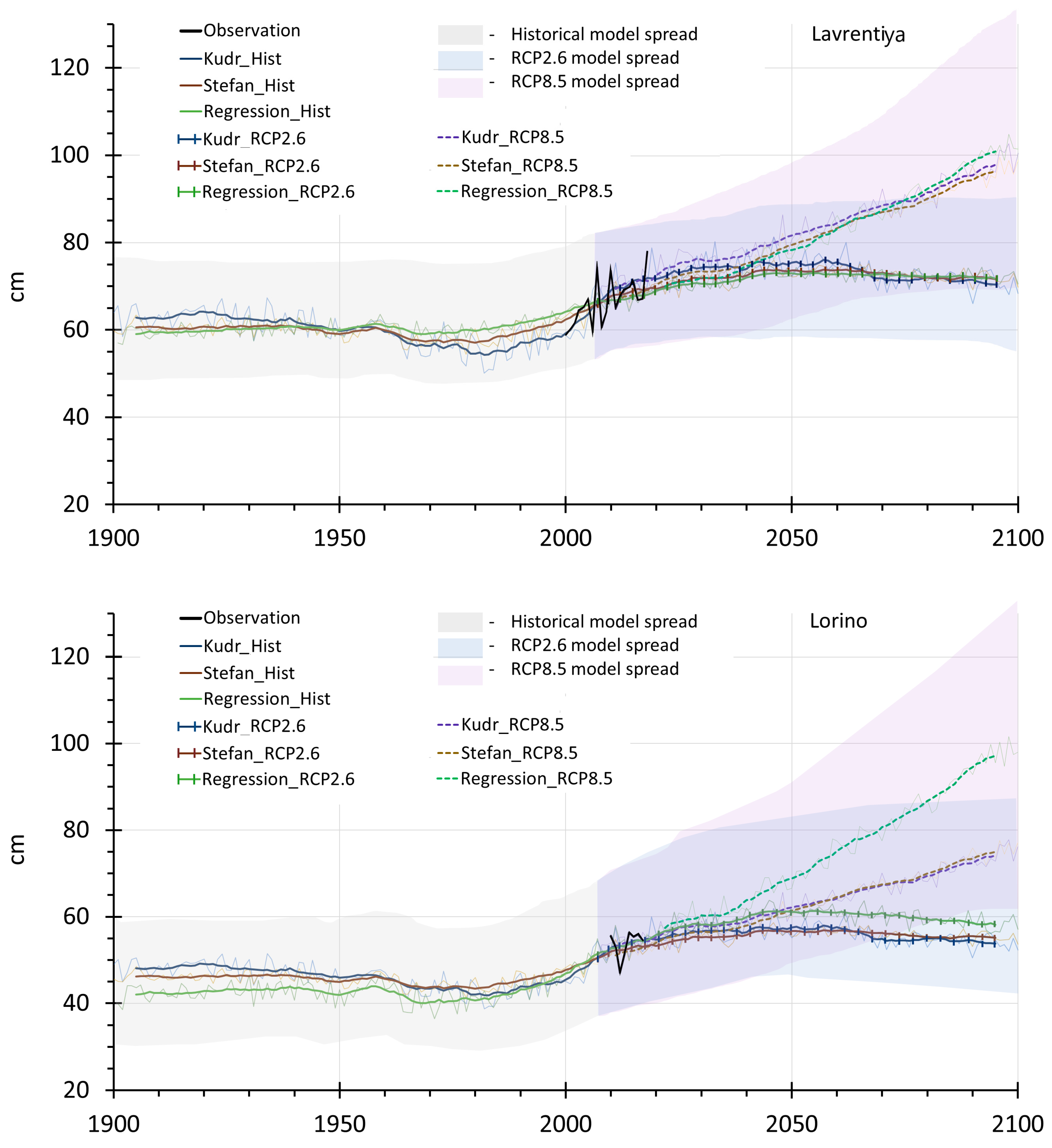
• Modeling of climatic parameters in the Chukotka region is associated with large uncertainties, probably caused by a lack of direct observations. The RMSE of the historical part of the ensemble of CMIP5 models and reanalysis is 7–20% for air temperatures and 22–33% for precipitation amounts. Thus, the climate in the study region is characterized by a wide range of possible values, that means that further calculations of ALT and thaw subsidence will be inaccurate. At the same time, the CMIP5 models ensemble reproduces some decadal fluctuations in air temperature (winter temperatures increase in the late 1990s—early 2000s, cooling from 2007, the general summer fluctuations). CMIP5 does not reproduce decadal fluctuations in the precipitation amount. In this case we can talk about the reproduction of mean annual (50–100 years) precipitation and use this data in construction of climate projections and the ALT. Based on CMIP5 climate reproduction, we should expect an increase in winter and summer temperatures and winter precipitation amounts in the 21st century. Under the positive scenario (RCP2.6), this growth will stop by 2050, under the negative one (RCP 8.5)—freezing and thawing indexes, precipitation amount in warm and cold periods will increase by 50−100% by the end of the century.
• The depth of seasonal thawing at the CALM sites Lavrentiya and Lorino, representing the natural conditions of the coastal plains of Eastern Chukotka, will increase by 6–13% by the end of the 21st century with a RCP 2.6 and by 43–87% with RCP 8.5.
• Active layer thickening will lead to irreversible surface subsidence, caused by permafrost thawing and ground ice melting. Under the RCP 2.6 climate scenario, the rate of surface lowering will be on average 0.4–1.5 cm·a⁻¹, and under RCP 8.5 1.6–3.7 cm·a⁻¹ (maximum 6.7 cm·a⁻¹) throughout the 21st century. Relative total settlement values by the end of the century will be 50–130% of the current ALT under the RCP 2.6 scenario to 300–500% of ALT under the RCP 8.5 scenario. The deposits of massive ice beds found near and at the CALM Lavrentiya site can trigger the formation of cryogenic erosional landforms, in particular, thaw slumps. According to various estimates, this can occur in the time interval from 2039 to 2085 depending on the model used for seasonal thawing and climate change scenarios.
• Both ALT increment and thaw subsidence will lead to a lowering of permafrost table. Depending on the natural conditions, the calculation approach and the climate change scenario, the total decline will have been from 150 to 310 cm by the end of the 21st century, and the main contribution to this process will be made by sediment thawing.
• Apparently, the formation of taliks due to the active layer thickening (non-merging permafrost) over the 21st century will not occur under any climate change scenario; however, at the RCP 8.5 scenario, the model spread for predicted ALT exceeds the values of potential seasonal freezing.
• The seasonal thawing models used in the article vary in plausibility and, as a result, give different predictive estimates. To increase the predictive accuracy, it is necessary to continue and expand monitoring observations of the parameters to determine the thermophysical properties of soil surface, seasonally thawing layer and the upper horizons of permafrost at the CALM sites as well as identify the influence of climatic characteristics on these properties. Another straightforward solution to improve the presented results is introducing numerical permafrost models.

References

1. Brown, R. The Distribution of Permafrost and Its Relation to Air Temperature in Canada and the U.S.S.R. ARCTIC 1960, 13, 163–177. [Google Scholar] [CrossRef]
2. Brown, J.; Ferrians, O.J., Jr.; Heginbottom, J.A.; Melnikov, E.S. Circum-Arctic Map of Permafrost and Ground-Ice Conditions; US Geological Survey: Reston, VA, USA, 1997; p. 45.
3. Kudryavtsev, V.A.; Dostovalov, B.N.; Romanovsky, N.N. General Geocryology; Publishing house MSU: Moscow, Russia, 1978; p. 464. (In Russian) [Google Scholar]
4. Streletskiy, D.A.; Tananaev, N.I.; Opel, T.; Shiklomanov, N.I.; Nyland, K.E.; Streletskaya, I.D.; Shiklomanov, A.I. Permafrost hydrology in changing climatic conditions: Seasonal variability of stable isotope composition in rivers in discontinuous permafrost. Environ. Res. Lett. 2015, 10, 095003. [Google Scholar] [CrossRef]
5. Schuur, E.A.G.; Bockheim, J.; Canadell, J.G.; Euskirchen, E.; Field, C.B.; Goryachkin, S.V.; Hagemann, S.; Kuhry, P.; LaFleur, P.M.; Lee, H.; et al. Vulnerability of Permafrost Carbon to Climate Change: Implications for the Global Carbon Cycle. BioScience 2008, 58, 701–714. [Google Scholar] [CrossRef]
6. Pavlov, A.V. Heat Exchange of Freezing and Thawing Grounds with the Atmosphere; Nauka: Moscow, Russia, 1965; p. 254. (In Russian) [Google Scholar]
7. Pavlov, A.V.; Gravis, G.F. Vechnaya merzlota i sovremennyy klimat [Permafrost and the modern climate]. Priroda 2000, 4, 10–17. [Google Scholar]
8. Kokelj, S.V.; Jorgenson, M.T. Advances in thermokarst research. Permafr. Periglac. Process. 2013, 24, 108–119. [Google Scholar] [CrossRef]
9. Shur, Y.L. The Upper Horizon of Permafrost and Thermokarst; Nauka: Novosibirsk, Russia, 1988; p. 209. (In Russian) [Google Scholar]
10. Hinkel, K.M.; Nelson, F.E. Spatial and temporal patterns of active layer thickness at Circumpolar Active Layer Monitoring (CALM) sites in northern Alaska, 1995–2000. J. Geophys. Res. Biogeosci. 2003, 108. [Google Scholar] [CrossRef]
11. Shur, Y.L.; Jorgenson, M.T. Patterns of permafrost formation and degradation in relation to climate and ecosystems. Permafr. Periglac. Process. 2007, 18, 7–19. [Google Scholar] [CrossRef]
12. Jorgenson, M.T.; Romanovsky, V.; Harden, J.; Shur, Y.; O’Donnell, J.; Schuur, E.A.; Kanevskiy, M.; Marchenko, S. Resilience and vulnerability of permafrost to climate change. Can. J. Forest Res. 2010, 40, 1219–1236. [Google Scholar] [CrossRef]
13. Hjort, J.; Karjalainen, O.; Aalto, J.; Westermann, S.; Romanovsky, V.E.; Nelson, F.E.; Etzelmüller, B.; Luoto, M. Degrading permafrost puts Arctic infrastructure at risk by mid-century. Nat. Commun. 2018, 9, 5147. [Google Scholar] [CrossRef] [PubMed]
14. Shiklomanov, N.I.; Streletskiy, D.A.; Swales, T.B.; Kokorev, V.A. Climate change and stability of urban infrastructure in Russian permafrost regions: Prognostic assessment based on GCM climate projections. Geogr. Rev. 2017, 107, 125–142. [Google Scholar] [CrossRef]
15. Streletskiy, D.A.; Shiklomanov, N.I.; Nelson, F.E. Permafrost, Infrastructure, and Climate Change: A GIS-Based Landscape Approach to Geotechnical Modeling. Arct. Antarct. Alp. 2012, 44, 368–380. [Google Scholar] [CrossRef] [Green Version]
16. Aalto, J.; Karjalainen, O.; Hjort, J.; Luoto, M. Statistical Forecasting of Current and Future Circum-Arctic Ground Temperatures and Active Layer Thickness. Geophys. Lett. 2018, 45, 4889–4898. [Google Scholar] [CrossRef] [Green Version]
17. Streletskiy, D.A.; Shiklomanov, N.I.; Nelson, F.E. Spatial variability of permafrost active-layer thickness under contemporary and projected climate in Northern Alaska. Polar Geogr. 2012, 35, 95–116. [Google Scholar] [CrossRef]
18. Nicolsky, D.J.; Romanovsky, V.E.; Panda, S.K.; Marchenko, S.S.; Muskett, R.R. Applicability of the ecosystem type approach to model permafrost dynamics across the Alaska North Slope. J. Geophys. Res. Earth Surf. 2017, 122, 50–75. [Google Scholar] [CrossRef]
19. Zhang, Y.; Li, J.; Wang, X.; Chen, W.; Sladen, W.; Dyke, L.; Dredge, L.; Poitevin, J.; McLennan, D.; Stewart, H.; et al. Modelling and mapping permafrost at high spatial resolution in Wapusk National Park, Hudson Bay Lowlands. Can. J. Earth Sci. 2012, 49, 925–937. [Google Scholar] [CrossRef]
20. Biskaborn, B.K.; Lanckman, J.-P.; Lantuit, H.; Elger, K.; Streletskiy, D.; Cable, W.L.; Romanovsky, V. The new database of the Global Terrestrial Network for Permafrost (GTN-P). Earth Sci. Data 2015, 7, 245–259. [Google Scholar] [CrossRef] [Green Version]
21. Stocker, T.F.; Qin, D.; Plattner, G.-K.; Tignor, M.M.B.; Allen, S.K.; Boschung, J.; Nauels, A.; Xia, Y.; Bex, V.; Midgley, P.M. IPCC, 2013: Climate Change 2013: The Physical Science Basis. Contribution of Working Group I to the Fifth Assessment Report of the Intergovernmental Panel on Climate Change; Cambridge University Press: Cambridge, UK; New York, NY, USA, 2013; p. 1535. [Google Scholar]
22. Anisimov, O.A.; Lobanov, V.A.; Reneva, S.A.; Shiklomanov, N.I.; Zhang, T.; Nelson, F.E. Uncertainties in gridded air temperature fields and effects on predictive active layer modeling. J. Geophys. Res. Biogeosci. 2007, 112, 112. [Google Scholar] [CrossRef]
23. Porter, C.; Morin, P.; Howat, I.; Noh, M.-J.; Bates, B.; Peterman, K.; Keesey, S.; Schlenk, M.; Gardiner, J.; Tomko, K.; et al. ArcticDEM. Available online: https://doi.org/10.7910/DVN/OHHUKH (accessed on 1 March 2019).
24. Gasanov, S. Structure and Formation History of Permafrost of Eastern Chukotka; Nauka: Moscow, Russia, 1969; p. 168. (In Russian) [Google Scholar]
25. Ivanov, V.F. Quaternary Sediments of Eastern Chukotka Coastal Area; DVNTS AN SSSR: Vladivostok, Russia, 1986; p. 140. (In Russian) [Google Scholar]
26. Kottek, M.; Grieser, J.; Beck, C.; Rudolf, B.; Rubel, F. World Map of the Köppen-Geiger climate classification updated. Meteorol. Z. 2006, 15, 259–263. [Google Scholar] [CrossRef]
27. Kobysheva, N.V. Climate of Russia; Hydrometizdat: Saint-Petersburg, Russia, 2001; p. 654. (In Russian) [Google Scholar]
28. Bulygina, O.N.; Razuvayev, V.N.; Trofimenko, L.T.; Shvets, N.V. Automated Information System for Processing Regime Information (AISPRI). Available online: http://aisori.meteo.ru/ClimateR (accessed on 26 March 2019).
29. Kolesnikov, S.F.; Plakht, I.R. Chukchi region. In Regional Cryolithology; Popov, A.I., Ed.; Izd-vo MGU: Moscow, Russia, 1989; pp. 201–217. (In Russian) [Google Scholar]
30. Afanasenko, V.E.; Zamolotchikova, S.A.; Tishin, M.I.; Zuev, I.A. Northern-Chukchi region. In Geocryology of USSR. Eastern Siberia and Far East; Ershov, E.D., Ed.; Nedra: Moscow, Russia, 1989; pp. 280–293. (In Russian) [Google Scholar]
31. Brown, J.; Hinkel, K.M.; Nelson, F.E. The circumpolar active layer monitoring (calm) program: Research designs and initial results1. Polar Geogr. 2000, 24, 166–258. [Google Scholar] [CrossRef]
32. Circumpolar Active Layer Monitoring Network-CALM: Long-Term Observations of the Climate-Active Layer-Permafrost System. Available online: https://www2.gwu.edu/~calm/ (accessed on 26 March 2019).
33. Walker, D.A.; Raynolds, M.K.; Daniëls, F.J.; Einarsson, E.; Elvebakk, A.; Gould, W.A.; Katenin, A.E.; Kholod, S.S.; Markon, C.J.; Melnikov, E.S.; et al. The circumpolar Arctic vegetation map. J. Veg. Sci. 2005, 16, 267–282. [Google Scholar] [CrossRef]
34. Gruber, S. Derivation and analysis of a high-resolution estimate of global permafrost zonation. Cryosphere 2012, 6, 221–233. [Google Scholar] [CrossRef] [Green Version]
35. Nelson, F.E.; Outcalt, S.I. A Computational Method for Prediction and Regionalization of Permafrost. Arct. Alp. 1987, 19, 279–288. [Google Scholar] [CrossRef]
36. Kalnay, E.; Kanamitsu, M.; Kistler, R.; Collins, W.; Deaven, D.; Gandin, L.; Iredell, M.; Saha, S.; White, G.; Woollen, J.; et al. The NCEP/NCAR 40-Year Reanalysis Project. Am. Meteorol. Soc. 1996, 77, 437–471. [Google Scholar] [CrossRef] [Green Version]
37. Taylor, K.E.; Stouffer, R.J.; Meehl, G.A. An Overview of CMIP5 and the Experiment Design. Am. Meteorol. Soc. 2012, 93, 485–498. [Google Scholar] [CrossRef] [Green Version]
38. Professional Information and Analytical Resource Dedicated to Machine Learning, Pattern Recognition and Data Mining. Available online: http://www.machinelearning.ru (accessed on 26 March 2019).
39. Anisimov, O.; Shiklomanov, N.; Nelson, F. Variability of seasonal thaw depth in permafrost regions: A stochastic modeling approach. Ecol. Model. 2002, 153, 217–227. [Google Scholar] [CrossRef]
40. Riseborough, D.; Shiklomanov, N.; Etzelmüller, B.; Gruber, S.; Marchenko, S. Recent advances in permafrost modelling. Permafr. Periglac. Process. 2008, 19, 137–156. [Google Scholar] [CrossRef]
41. Bonnaventure, P.P.; Lamoureux, S.F. The active layer: A conceptual review of monitoring, modelling techniques and changes in a warming climate. Prog. Phys. Geogr. Earth 2013, 37, 352–376. [Google Scholar] [CrossRef]
42. Shiklomanov, N.I.; Nelson, F.E. Active-layer mapping at regional scales: a 13-year spatial time series for the Kuparuk region, north-central Alaska. Permafr. Periglac. Process. 2002, 13, 219–230. [Google Scholar] [CrossRef]
43. Kudryavtsev, V.A.; Garagula, L.S.; Kondrat’yeva, K.A. Fundamentals of Frost Forecasting in Geological Engineering Investigations; Izdatel’stvo MGU: Moscow, Russia, 1974; p. 430. (In Russian) [Google Scholar]
44. Romanovsky, V.E.; Osterkamp, T.E. Thawing of the Active Layer on the Coastal Plain of the Alaskan Arctic. Permafr. Periglac. Process. 1997, 8, 1–22. [Google Scholar] [CrossRef]
45. Sazonova, T.S.; Romanovsky, V.E. A model for regional-scale estimation of temporal and spatial variability of active layer thickness and mean annual ground temperatures. Permafr. Periglac. Process. 2003, 14, 125–139. [Google Scholar] [CrossRef]
46. Osterkamp, T.E.; Jorgenson, M.T.; Schuur, E.A.G.; Shur, Y.L.; Kanevskiy, M.Z.; Vogel, J.G.; Tumskoy, V.E. Physical and ecological changes associated with warming permafrost and thermokarst in Interior Alaska. Permafr. Periglac. Process. 2009, 20, 235–256. [Google Scholar] [CrossRef]
47. Morgenstern, A.; Ulrich, M.; Günther, F.; Roessler, S.; Fedorova, I.; Rudaya, N.; Wetterich, S.; Boike, J.; Schirrmeister, L.; Rudaya, N. Evolution of thermokarst in East Siberian ice-rich permafrost: A case study. Geomorphology 2013, 201, 363–379. [Google Scholar] [CrossRef]
48. Mazhitova, G.G.; Kaverin, D.A. Dynamics of the depth of seasonal thawing and precipitation of the soil surface at the circumpolar monitoring of the active layer (CALM) in the European part of Russia. Earth’s Cryosphere 2007, 11, 20–30. (In Russian) [Google Scholar]
49. Shiklomanov, N.I.; Streletskiy, D.A.; Little, J.D.; Nelson, F.E. Isotropic thaw subsidence in undisturbed permafrost landscapes. Geophys. Lett. 2013, 40, 6356–6361. [Google Scholar] [CrossRef]
50. Arzhanov, M.M.; Demchenko, P.F.; Eliseev, A.V.; Mokhov, I.I. Simulation of thawing sediments of permafrost in the northern hemisphere in the 21st century. Earth’s Cryosphere 2010, 14, 37–42. (In Russian) [Google Scholar]
51. Shur, Y.; Hinkel, K.M.; Nelson, F.E. The transient layer: implications for geocryology and climate-change science. Permafr. Periglac. Process. 2005, 16, 5–17. [Google Scholar] [CrossRef]
52. Maslakov, A.A.; Ruzanov, V.T.; Fedorov-Davydov, D.G.; Kraev, G.N.; Davydov, S.P.; Zamolodchikov, D.G.; Tregubov, O.D.; Shiklomanov, N.I.; Streletsky, D.A. Seasonal thawing of soils in Beringia in current climate change. Arct. Environ. Res. 2017, 17, 283–294. (In Russian) [Google Scholar] [CrossRef]
53. Abramov, A.A.; Davydov, S.P.; Ivashchenko, A.I.; Karelin, D.V.; Kholodov, A.L.; Kraev, G.N.; Lupachev, A.V.; Maslakov, A.A.; Ostroumov, V.E.; Rivkina, E.M.; et al. Two Decades of Active Layer Thickness Monitoring in Northeastern Asia. Polar Geography, accepted.
54. Parmuzin, S.Y.; Shatalova, T.Y. Dynamics of seasonally low and seasonally frozen layers of rocks due to short-period climate variations. In Fundamentals of Geocryology, Dynamic Geocryology; Ershov, E.D., Ed.; Izdatel’stvo MGU: Moscow, Russia, 2001; Volume 4, pp. 284–303. (In Russian) [Google Scholar]
55. Zamolodchikov, D.G.; Kotov, A.N.; Karelin, D.V.; Razzhivin, V.Y. Active-Layer Monitoring in Northeast Russia: Spatial, Seasonal, and Interannual Variability. Polar Geogr. 2004, 28, 286–307. [Google Scholar] [CrossRef]
56. Christiansen, H.H. Meteorological control on interannual spatial and temporal variations in snow cover and ground thawing in two northeast Greenlandic Circumpolar-Active-Layer-Monitoring(CALM) sites. Permafr. Periglac. Process. 2004, 15, 155–169. [Google Scholar] [CrossRef]
57. Karelin, D.V.; Zamolodchikov, D.G. Carbon Exchange in Cryogenic Ecosystems; Nauka: Moscow, Russia, 2008; p. 344. (In Russian) [Google Scholar]
58. Garagulya, L.S. Potential seasonal freezing and potential seasonal thawing of rocks. In Fundamentals of Geocryology, Dynamic Geocryology; Ershov, E.D., Ed.; Izdatel’stvo MGU: Moscow, Russia, 2001; Volume 4, pp. 253–258. (In Russian) [Google Scholar]
59. Jafarov, E.; Marchenko, S.S.; Romanovsky, V.E. Numerical modeling of permafrost dynamics in Alaska using a high spatial resolution dataset. Cryosphere 2012, 6, 613–624. [Google Scholar] [CrossRef] [Green Version]
Figure 1. Location of active layer monitoring sites. Permafrost zonation index (PZI) and glaciers extent are derived from [34].
Geosciences 09 00232 g001
Figure 2. Aerial photos of the Circumpolar Active Layer Monitoring (CALM) sites made from UAV (Unmanned aerial vehicle) in 2018.
Geosciences 09 00232 g002
Figure 3. Areas of reanalysis and climate models data averaging. Red rectangle marks CALM sites location.
Geosciences 09 00232 g003
Figure 4. Thaw (It) and frost (If) indexes, summer and winter precipitation amounts, and seasonal thaw depths at Lavrentiya and Lorino CALM sites variations for 2000–2017.
Geosciences 09 00232 g004
Figure 5. Thaw subsidence and frost heave dynamics for 2012–2018 on Lavrentiya CALM site. ALT (purple bars) is given as averaged value for the whole site.
Geosciences 09 00232 g005
Figure 6. Interrelation of measured active layer thickness and square root of thawing index on the CALM sites of Eastern Chukotka.
Geosciences 09 00232 g006
Figure 7. Comparison of measured ALT with the ones modeled with regression, Stefan and Kudryavtsev methods for the Lavrentiya and Lorino sites. Grey lines confine the standard deviations for measured values.
Geosciences 09 00232 g007
Figure 8. Historical and projected ALT dynamics for the Lavrentiya (upper) and Lorino (lower) CALM sites based on 3 models and RCP 2.6 and 8.5 climatic scenarios. The uncertainty bound (model spread) is calculated as described in Section 3.3.
Geosciences 09 00232 g008
Figure 9. Thaw subsidence projections at Lavrentiya and Lorino CALM sites for 2017–2100 based on 3 active layer thickness models and RCP 2.6 and 8.5 climatic scenarios. The uncertainty bound is calculated as described in Section 3.4.
Geosciences 09 00232 g009