The Optimal Location of Ground-Based GNSS Augmentation Transceivers

Abstract

Modern Global Navigation Satellite Systems (GNSS) allow for positioning with accuracies ranging from tens of meters to single millimeters depending on user requirements and available equipment. A major disadvantage of these systems is their unavailability or limited availability when the sky is obstructed. One solution is to use additional range measurements from ground-based nodes located in the vicinity of the receiver. The highest accuracy of distance measurement can be achieved using ultra wide band (UWB) or ZigBee phase shift measurement. The position of the additional transmitter must be carefully selected in order to obtain the optimal improvement in the dilution of precision (DOP), which reflects the improvement in the geometry of solution. The presented case study depicts a method for selecting the optimal location of a ground-based ranging source. It is based on a search of a minimum DOP value as a transmitter location function. The parameters of objective function are the elevation and azimuth of the transceiver. The solution was based on a limited-memory Broyden–Fletcher–Goldfarb–Shanno with Box constraints (L-BFGS-B) method and a numerical optimization algorithm for parameter value estimation. The presented approach allows for the selection of the optimal location of a ground-based source of ranging signals in GNSS processing from a geometry of solution point of view. This can be useful at the design stage of an augmentation network of ground-based transceivers. This article presents a theoretical basis and a case study presenting the selection of the optimal location of a ground-based ranging source.

1. Introduction

Modern Global Navigation Satellite Systems (GNSS) allow for positioning with accuracies ranging from tens of meters to single millimeters depending on user requirements and available equipment. A major disadvantage of these systems is their unavailability or limited availability when the sky is obstructed. A GNSS signal level at the receiver is about −130 dBm. This is the main reason why line of sight (LOS) propagation is required. Even if only part of the sky is obstructed, an unfavorable distribution of satellites can result in substantial positioning uncertainty, reflected in the large dilution of precision (DOP) parameter values.

To mitigate this problem and to allow for positioning in unfavorable conditions, local area ground-based augmentation of GNSS can be introduced. In many cases these systems provide an improvement in accuracy by correcting the GNSS observables in order to eliminate the impact of common errors (ephemeris and satellite clock errors and ionospheric and tropospheric delays) [1]. Another solution is to use additional range measurement from ground-based nodes located in the vicinity of the receiver. To achieve this task many technologies can be used: pseudolites, Ultra Wide Band (UWB), or distance measurement using modern communication networks such as WiFi, Bluetooth, or ZigBee. In these networks the distance can be obtained using various techniques: the radio signal strength indicator (RSSI), the time of flight (TOF), the time of arrival (TOA), or the differential time of arrival (TDOA) [2,3]).

The above-mentioned technologies vary in accuracy, range, scale, and data rate. The highest accuracy of distance measurement (about 10 cm) can be achieved using UWB or ZigBee phase shift measurement [4], which gives the opportunity to use the phase measurement unit of a ZigBee chip to improve the precision of the distance measurement [5]. A comprehensive study of these technologies can be found in [6].

Regardless of the distance measurement technology, additional distance observation should result in geometry improvement, which can be evaluated using DOP factors [7]. The position of the additional transmitter must be carefully selected in order to obtain the optimal DOP value (understood as its maximum possible improvement referenced to the DOP value without augmentation transceiver). In this paper, the method of selecting the optimal location of ranging source selection is presented. It is based on a search of a minimum DOP value as a transmitter location function.

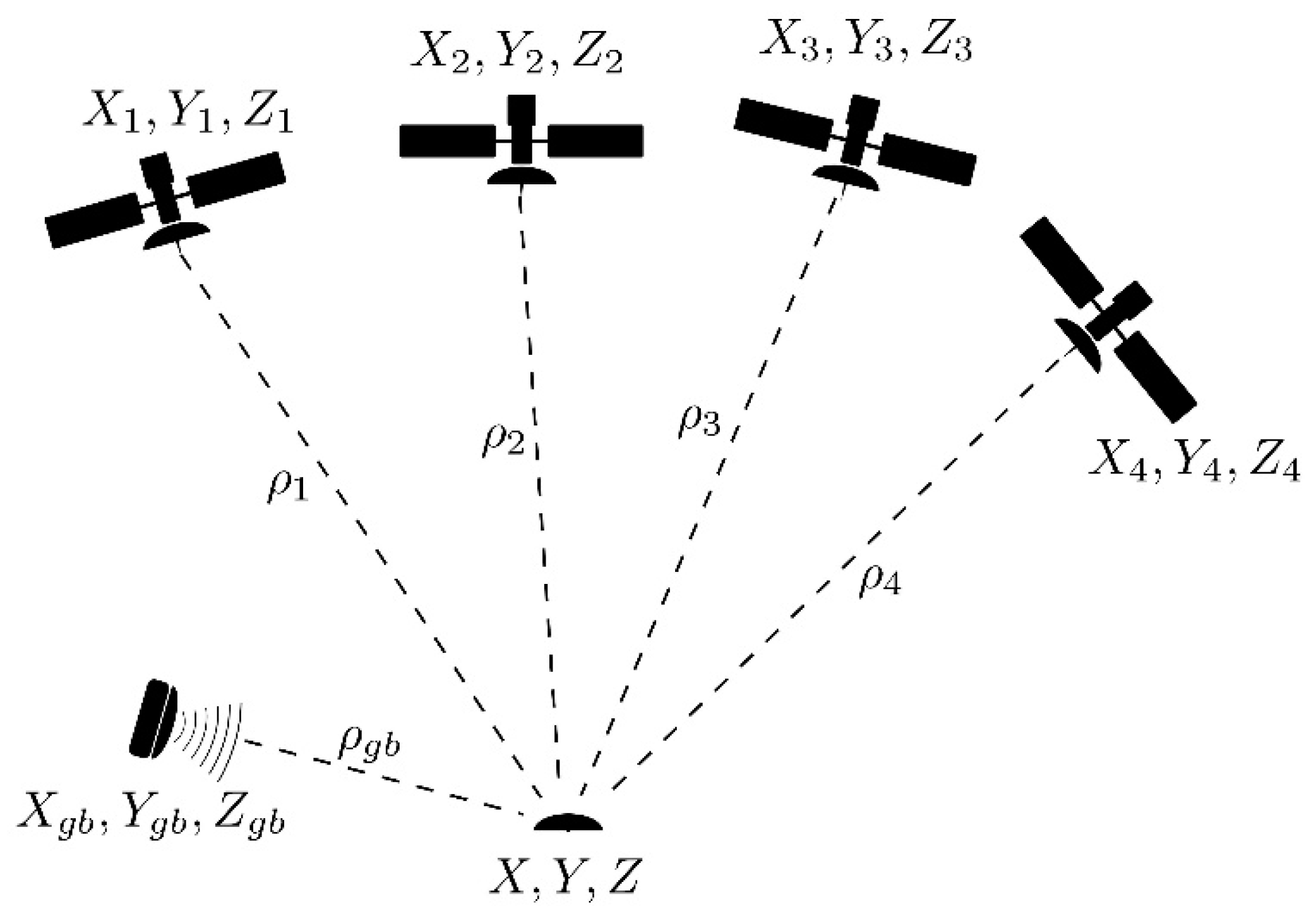
2. Calculation of DOP Values

Simplified geometry of GNSS single point positioning augmented with ground-based distance measurement is depicted in Figure 1. Dilution of precision is a factor describing the multiplicative effect of navigation satellite geometry on positional measurement precision. It can be calculated in different variants depending on the component we want to describe. Most common are

• geometric dilution of precision (GDOP);
• position (3D) dilution of precision (PDOP);
• time dilution of precision (TDOP)

Using symbols from Figure 1 and a GNSS-only situation, the covariance matrix of single point positioning can be defined as

$$Q={(G^{T}G)}^{-1}=\left[\begin{array}{cccc}{\sigma }_X^2& {\sigma }_{XY}& {\sigma }_{XZ}& {\sigma }_{Xt}\\ {\sigma }_{XY}& {\sigma }_Y^2& {\sigma }_{YZ}& {\sigma }_{Yt}\\ {\sigma }_{XZ}& {\sigma }_{YZ}& {\sigma }_Z^2& {\sigma }_{Zt}\\ {\sigma }_{Xt}& {\sigma }_{Yt}& {\sigma }_{Zt}& {\sigma }_t^2\end{array}\right],$$

(1)

and the design matrix for single point positioning, derived from the partial derivative for each receiver satellite pseudorange ρ_i, is

$$G=\left[\begin{array}{cccc}{g}_{1X}& g_{1Y}& g_{1Z}& 1\\ g_{2X}& g_{2Y}& g_{2Z}& 1\\ g_{3X}& g_{3Y}& g_{3Z}& 1\\ & ⋮& & \\ g_{nX}& g_{nY}& g_{nZ}& 1\end{array}\right].$$

(2)

The terms X, Y, and Z in Equation (2) are components of unit vectors from the receiver to each satellite, and 1 stands for the receiver clock correction:

$$g_{iX}=\frac{x_i-X}{{\rho }_i}\hspace{1em}{g}_{iY}=\frac{y_i-Y}{{\rho }_i}\hspace{1em}{g}_{iZ}=\frac{z_i-Z}{{\rho }_i}$$

(3)

where x_i, y_i, and z_i are satellite coordinates, X, Y, and Z are receiver coordinates, and ρ_i is a receiver–satellite distance. The terms in Equation (3) are the first terms of the Taylor series expansion of range equation. Usually distances in the denominator are calculated on the basis of satellite coordinates and approximate coordinates of the receiver. Increments to approximate coordinates are then calculated using least squares (in positioning application). DOP factors can be defined as follows.

Geometric dilution of precision:

$$GDOP=\sqrt{{\sigma }_X^2+{\sigma }_Y^2+{\sigma }_Z^2+{\sigma }_t^2}.$$

(4)

Position (3D) dilution of precision:

$$PDOP=\sqrt{{\sigma }_X^2+{\sigma }_Y^2+{\sigma }_Z^2}.$$

(5)

Time dilution of precision:

$$TDOP=\sqrt{{\sigma }_t^2}.$$

(6)

Adding a ground-based range observation yields the following form of design matrix G:

$$G=\left[\begin{array}{cccc}{g}_{1X}& g_{1Y}& g_{1Z}& 1\\ g_{2X}& g_{2Y}& g_{2Z}& 1\\ g_{3X}& g_{3Y}& g_{3Z}& 1\\ & ⋮& & \\ g_{nX}& g_{nY}& g_{nZ}& 1\\ w_{gbX}& w_{gbY}& w_{gbZ}& 0\end{array}\right]$$

(7)

where:

$$w_{gbX}=\frac{x_{gb}-X}{{\rho }_{gb}}\hspace{1em}{w}_{gbY}=\frac{y_{gb}-Y}{{\rho }_{gb}}\hspace{1em}{w}_{gbZ}=\frac{z_{gb}-Z}{{\rho }_{gb}},$$

(8)

and ρ_gb is the approximate receiver–augmentation transceiver distance.

UWB or ZigBee ground-based observations does not depend on the receiver clock so the last term in the G matrix is equal to 0. This means that the change in GDOP will be the same as the change in PDOP. In general, we are interested in 3D navigation, so VDOP and HDOP are less important than PDOP. The next part of this paper is focused only on the PDOP factor. The principles of measuring distance with UWB or ZigBee are described in [4,5,8,9].

3. DOP Optimization Strategy

The location of additional ground-based transceivers should be selected in a way that will optimize the DOP improvement, taking into account local conditions (such as the abilities to mount the transceiver antenna or local obstructions of the sky). In order to obtain information about local obstructions, a laser scanning technology can be used. In relation to this, studies on the modeling of the surrounding space based on laser scanning can be useful [10,11]. For all transmitter positions in the transceiver–receiver unit vector direction, PDOP factor values will be the same. This unit vector can be calculated using the azimuth (Az) and elevation (El) of the transmitter in a topocentric coordinate frame.

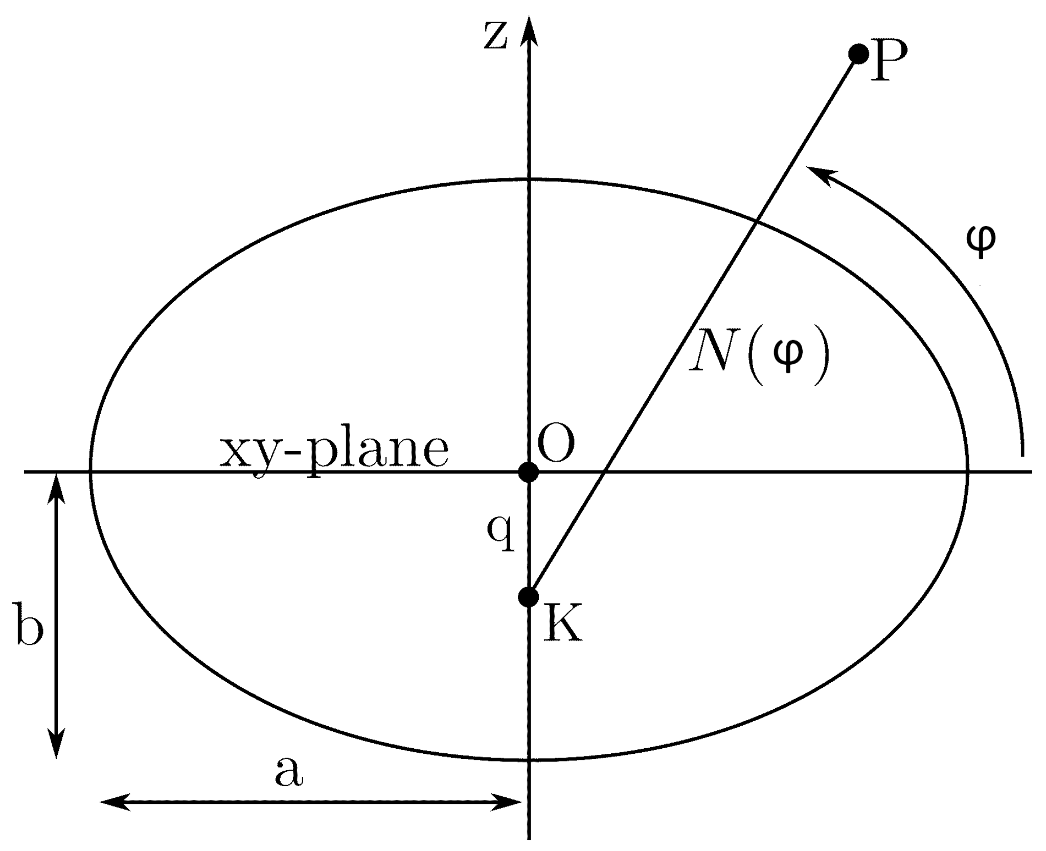
3.1. Coordinate Transformation

To transform the satellite coordinates to the topocentric coordinate frame, the following steps were performed:

1. Calculation of geodetic satellite coordinates (latitude φ, longitude λ, height h), and distance q from the center of the ellipsoid to the intersection of the normal to the ellipsoid at the receiver position (Figure 2) [12].

This was done using an iterative algorithm:

$$N(\phi )=\frac{a}{\sqrt{1-{(esin({\phi }_{old}))}^2}}$$

(9)

$$q=N(\phi )e^2\sin ({\phi }_{old})$$

(10)

$$r=\sqrt{x^2+y^2}$$

(11)

$$\phi =\arctan \frac{z+q}{r}$$

(12)

$${\phi }_{old}=\phi .$$

(13)

The iterative process stops when

$$|\phi -{\phi }_{old}|<\frac{1^{″}}{100}.\mathrm{Then}:\lambda =\arcsin \frac{y}{r}.$$

(14)

2. Translation of the receiver and satellite positions by q in the z direction:

$$\left[\begin{array}{c}X\\ Y\\ Z\end{array}\right]=\left[\begin{array}{c}x\\ y\\ z\end{array}\right]+\left[\begin{array}{c}0\\ 0\\ q\end{array}\right].$$

(15)

3. Rotation around the Z and Y axes—Equations (16) and (17), respectively [13]:

$$\left[\begin{array}{c}{X}^{\prime }\\ Y^{\prime }\\ Z^{\prime }\end{array}\right]=\left[\begin{array}{ccc}\cos \left(-\lambda \right)& \sin \left(-\lambda \right)& 0\\ \sin \left(-\lambda \right)& \cos \left(-\lambda \right)& 0\\ 0& 0& 1\end{array}\right]\left[\begin{array}{c}X\\ Y\\ Z\end{array}\right]$$

(16)

$$\left[\begin{array}{c}{X}^{″}\\ Y^{″}\\ Z^{″}\end{array}\right]=\left[\begin{array}{ccc}\cos \left(-\phi \right)& 0& \sin \left(-\phi \right)\\ 0& 1& 0\\ \sin \left(-\phi \right)& 0& \cos \left(-\phi \right)\end{array}\right]\left[\begin{array}{c}{X}^{\prime }\\ Y^{\prime }\\ Z^{\prime }\end{array}\right].$$

(17)

Translation by the semi minor axis in the z direction:

$$\left[\begin{array}{c}{X}_{local}\\ Y_{local}\\ Z_{local}\end{array}\right]=\left[\begin{array}{c}{X}^{″}\\ Y^{″}\\ Z^{″}\end{array}\right]+\left[\begin{array}{c}0\\ 0\\ -b\end{array}\right].$$

(18)

After completing the above steps, the coordinates of all satellites are in the topocentric coordinate frame with its origin at the receiver position. According to Equation (19), the Cartesian coordinates of the transceiver located at a particular elevation (El) and azimuth (Az) and at distance equal to 1 can be calculated:

$$\left[\begin{array}{c}{X}^{″}{}_{gb}\\ Y^{″}{}_{gb}\\ Z^{″}{}_{gb}\end{array}\right]=\left[\begin{array}{c}\cos \left(El\right)\sin \left(Az\right)\\ \cos \left(El\right)\cos \left(Az\right)\\ \sin \left(El\right)\end{array}\right].$$

(19)

3.2. Objective Function

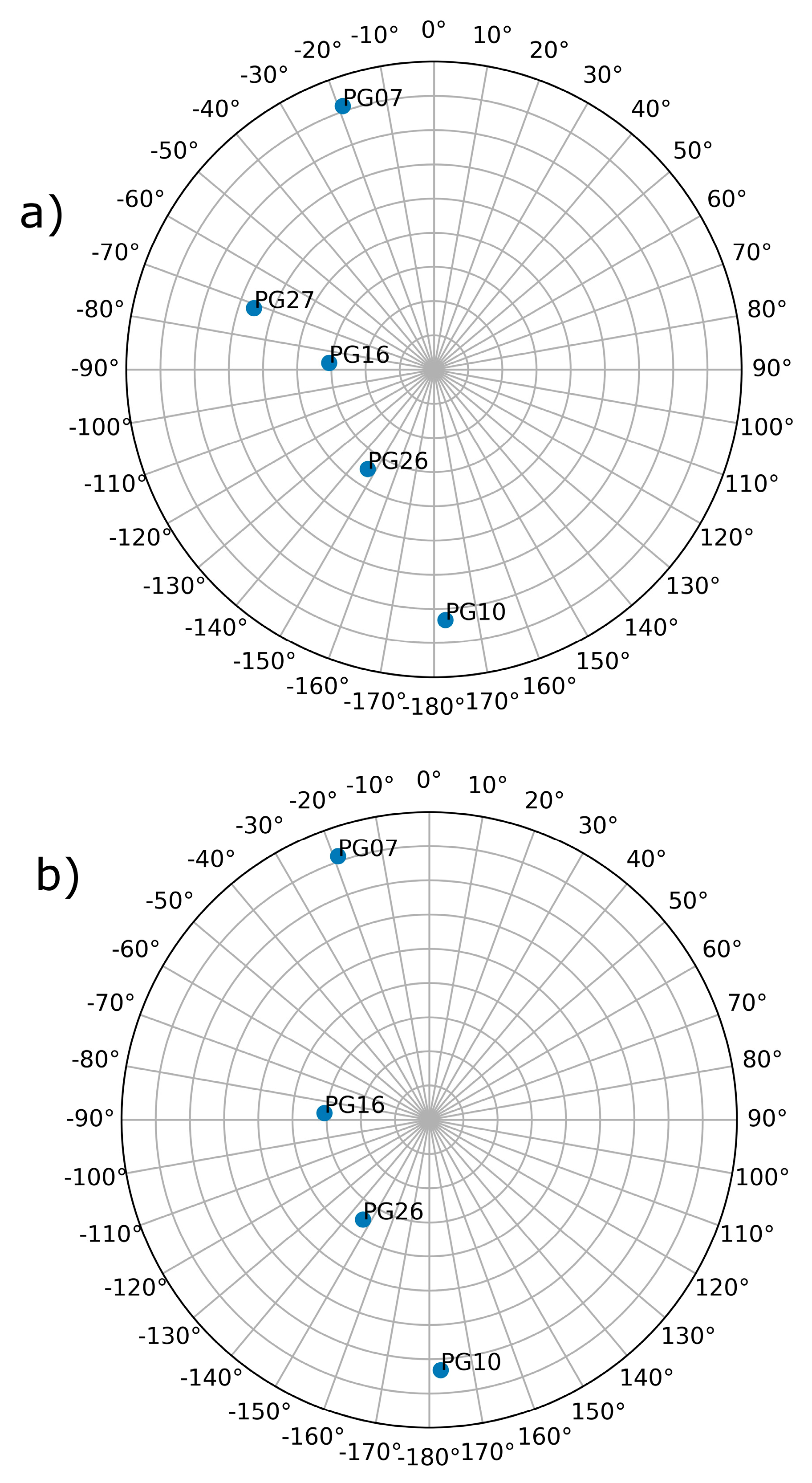
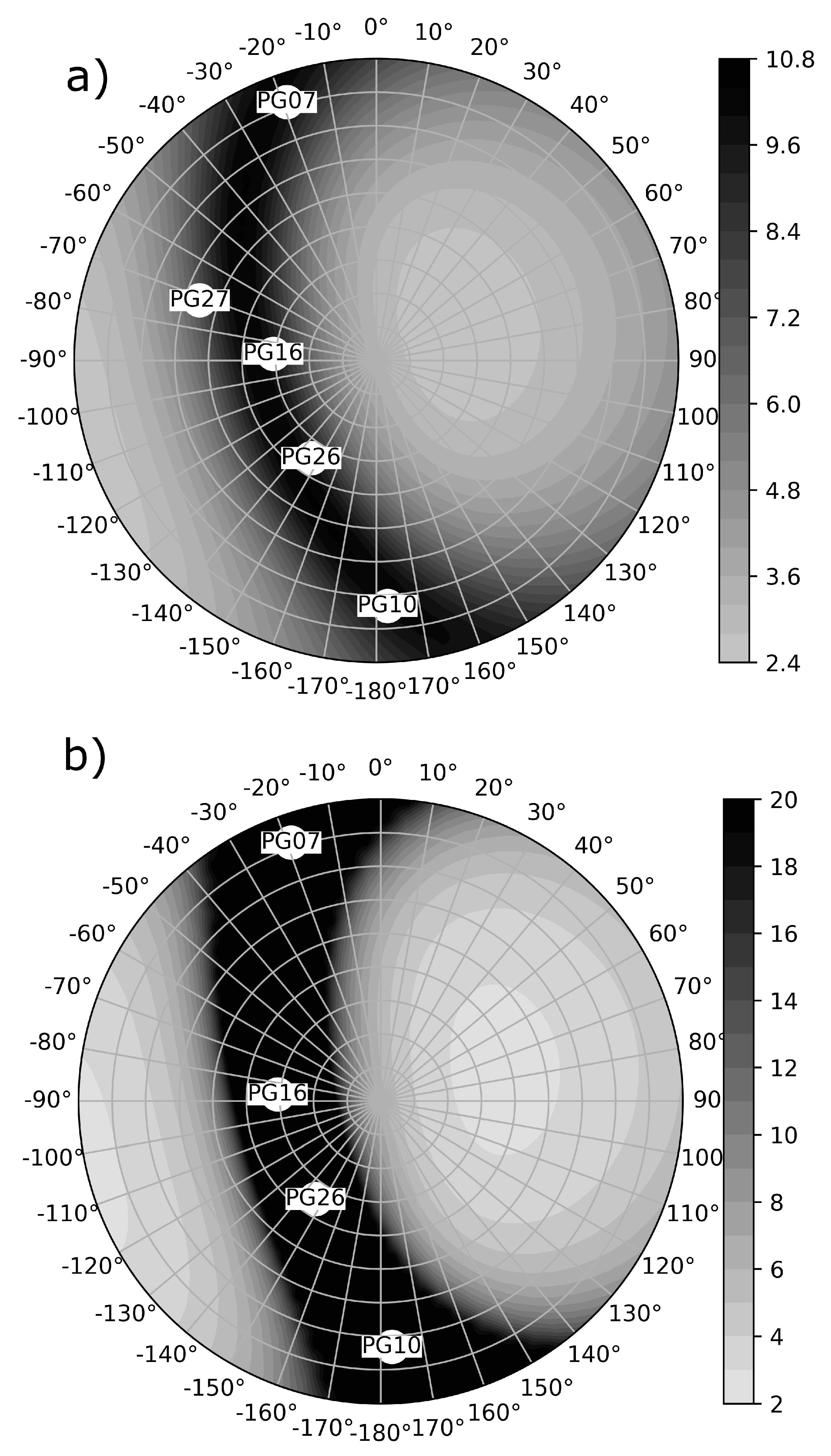
The main objective of PDOP minimization is to find the elevation and azimuth of the transceiver, which will minimize the PDOP value:

argmin(PDOP(El, Az)).

(20)

In order to calculate solution of this function, one of the numerical methods can be used. As described in [14], the mathematical minimum of such function results with satellites distributed uniformly around the receiver. This means that an additional transmitter would have to be located with the elevation lower than 0. This is the reason why the selected method should allow one to define constraints on the parameters (El, Az). The L-BFGS-B method [15,16] for optimal position estimation was chosen for this problem. This is a modification of the limited-memory BFGS optimization algorithm. It belongs to the family of quasi Newton methods and approximates the Broyden–Fletcher–Goldfarb–Shanno algorithm. The modification allows one to handle bound constraints on variables. In our case, the parameters are constrained as follows:

Az ∈ < 0°;360° > El ∈ < 0°; 60° >.

(21)

The above-mentioned constraints limit the result of the algorithm to transmitter locations above the horizon. Maximum elevation is equal to 60° due to the technical difficulties of placing the transmitter high above the ground.

As a quasi-Newton method, the BFGS and all of its modifications, is an iterative method.

$$x_{k+1}=x_k-{\alpha }_k{H}_k{g}_k$$

(22)

where x_k and x_k+1 are two consecutive approximations of function parameters, H_k is approximation to the inverse Hessian, g_k is a gradient, and α_k is a step size. In BFGS, defining

$${\delta }_k=x_{k+1}-x_k$$

(23)

and

$${\gamma }_k=g_{k+1}-g_k,$$

(24)

the matrix H_k+1 is updated using Equation (25).

$$H_{k+1}=H_k-\frac{{\delta }_k{\gamma }_k^T{H}_k+H_k{\gamma }_k{\delta }_k^T}{{\delta }_k^T{\gamma }_k}+\left(1+\frac{{\gamma }_k^T{H}_k{\gamma }_k}{{\delta }_k^T{\gamma }_k}\right)\frac{{\delta }_k{\delta }_k^T}{{\delta }_k^T{\gamma }_k}.$$

(25)

In order to determine the step size α_k, a Wolfe line search is usually used [17]. Limited-memory–BFGS (L-BFGS) is a less computationally expensive variation of the method [18]. In this modification, instead of updating and storing the entire approximated inverse Hessian, the information from the past m iterations is stored. This information is used to compute the next search direction. It is of particular importance when the number of dimensions of the objective function is large.

For the calculations presented in the case study, the SciPy implementation of the method was used [19].

4. Case Study

For the case study, we placed the receiver on a street between two buildings at the University of Warmia and Mazury in Olsztyn, Poland. Satellite locations were calculated on the basis of precise orbits from 20 May 2016 at 18:00. The location of the receiver and obstacles in the vicinity caused the receiver to track only five satellites, depicted in the bottom panel of Figure 3. To perform tests in even worse conditions, satellite PG27 was removed from the constellation (Figure 3a).

The location is a typical urban canyon with high buildings on both sides of the road. As a result, for the case with five satellites, PDOP factors were 10.35 and 797.64 for the case with four satellites. A very large value of PDOP for the case with four satellites was caused by the collinear alignment of satellites in view. Both situations are not satisfactory for reliable positioning. Improvement of the PDOP factor after adding a ground-based transmitter depends on the transmitter’s location. To depict the distribution of the PDOP-dependent transmitter’s elevation and azimuth, PDOP values were calculated for a given transceiver’s azimuth and elevation in a four-degree grid. Results are depicted, for the case with five satellites, in the bottom panel of Figure 4 and, for the case with four satellites, in the top panel of Figure 4. For readability, the PDOP value above 20 was masked and is displayed as 20.

Figure 5 depicts the route that the L-BFGS-B algorithm takes in order to determine the optimal location of the ground-based transmitter. The algorithm requires the initial location of the transceiver to be provided a priori. The initial location was selected in four places, namely in the northeast (NE), southeast (SE), southwest (SW), and northwest (NW). In the case of an urban canyon, the distribution of the satellites is usually more or less collinear. This causes the optimal transceiver location to lay “on both sides of the street.” Selecting four initial positions allows one to find those two locations. In the presented case study, the algorithm resulted in two locations—one on the east side and one on the west side. The result for the SE and NE was on the east side with an elevation of approximately 53°. The other solution was on the west side, low above the horizon, at an approximately 0° elevation.

The value of the PDOP function at each step of the algorithm is described in

Table 1. Function values at iterations.

	Initial Position
Iteration	NE	SE	SW	NW
0	3.75	5.58	16.54	34.41
1	3.11	5.86	12.53	12.53
2	2.91	4.66	7.98	7.98
3	2.76	3.23	6.20	6.20
4	2.75	2.98	4.64	4.64
5		2.83	3.72	3.72
6		2.75	3.12	3.12
7		2.75	2.82	2.82
8			2.76	2.76
9			2.75	2.75
10			2.75	2.75
11			2.75	2.75

.

Table 2. Summary of the algorithm.

	Initial Position
	NE	SE	SW	NW
Number of iterations	4	7	11	11
Number of function evaluations	18	28	13	13
Number of segments explored during Cauchy searches	5	8	13	13
Number of BFGS updates skipped	0	0	0	0
Number of active bounds at final generalized	0	0	1	1
Cauchy point norm of the final projected gradient	0.27	2.64	1.12 × 10−8	1.12 × 10−8
Final function value	2.75	2.75	2.75	2.75

gives the overall summary of the iterative process of the LBFGS-B estimation. The algorithm finished at most of the 11 iterations with a 2.75 PDOP value in all cases. The resulting PDOP value in the last few iterations was equal to one hundredth. This indicates that the region with a PDOD equal to 2.75 is relatively large and “flat.” It is represented as the lightest color in Figure 5. Figure 3, Figure 4 and Figure 5 are heat maps in the polar coordinate system. The distance from the center depicts elevation, the angle depicts azimuth, and the PDOP (Figure 4 and Figure 5) value is presented in color.

5. Conclusions

In this paper, we define the optimal location of a GNSS augmentation transceiver as a minimum of PDOP function. PDOP values were calculated using satellite geometry and transceiver elevation and azimuth. The augmentation transceiver can be any ranging source—from robotic total station to pseudolite. The proposed approach can be useful at the design stage of the local area augmentation system based on additional ranging measurements. A similar approach can be utilized for more than one location of the receiver and more than one transceiver. The process can be repeated for many places in the area where the sky is obstructed, and the optimal location of transceivers can be selected. The approach is similar to the one presented in [7]. The area considered for augmentation can be covered with a grid of simulated receiver locations. Computations can then be repeated for each location, and the optimal position of transceiver can be stored as an array. Finally, a clustering algorithm can be used to select the best location for the entire area.

This approach is also valid for range-based indoor navigation, when the network of ranging sensors must be densified. The application of an L-BFGS-B optimization method allows for constraints on selected parameters. This is a means by which one can limit the location of the transceiver to accessible locations that might be, for example, on the wall of a building or a given required height.

It is worth highlighting that a ground-based augmentation system (GBAS) from 2007 has been standardized by the International Civil Aviation Organization (ICAO) to provide precision approach navigation services using the GNSS [20].

References

1. Braff, R.; Shively, C. A method of over bounding ground-based augmentation system (GBAS) heavy tail error distributions. J. Navig. 2005, 58, 83103. [Google Scholar] [CrossRef]
2. Chen, Q.; Liu, H.; Yu, M.; Guo, H. RSSI Ranging Model and 3D Indoor Positioning with ZigBee Network. In Proceedings of the 2012 IEEE/ION Position Location and Navigation Symposium (PLANS), Myrtle Beach, SC, USA, 23–26 April 2012; pp. 1233–1239. [Google Scholar] [CrossRef]
3. Farid, Z.; Nordin, R.; Ismail, M. Recent advances in wireless indoor localization techniques and system. J. Comput. Netw. Commun. 2013, 2013, 185138. [Google Scholar] [CrossRef]
4. Rapinski, J.; Cellmer, S. Analysis of Range Based Indoor Positioning Techniques for Personal Communication Networks. Mob. Netw. Appl. 2016, 21, 539–549. [Google Scholar] [CrossRef]
5. Rapinski, J.; Smieja, M. ZigBee Ranging using Phase Shift Measurements. J. Navig. 2015, 68, 665–677. [Google Scholar] [CrossRef] [Green Version]
6. Koyuncu, H.; Shuang, H. A survey of indoor positioning and object locating systems, IJCSNS International. J. Comput. Sci. Netw. Secur. 2010, 10, 121–128. [Google Scholar]
7. Janowski, A.; Rapinski, J. The analyzes of PDOP factors for a ZigBee groundbased augmentation systems. Pol. Marit. Res. 2017, 24, 108–114. [Google Scholar] [CrossRef]
8. Sahinoglu, Z.; Gezici, S.; Guvenc, I. Ultra-wideband Positioning Systems: Theoretical Limits, Ranging Algorithms, and Protocols; Cambridge University Press: Cambridge, UK, 2008; ISBN 9780521873093. [Google Scholar]
9. Rapinski, J. The application of ZigBee phase shift measurement in ranging. Acta Geodyn. Geomater. 2015, 12, 291780. [Google Scholar] [CrossRef]
10. Bobkowska, K.; Inglot, A.; Mikusova, M.; Tysiąc, P. Implementation of Spatial Information for Monitoring and Analysis of the Area Around the Port Using Laser Scanning Techniques. Pol. Marit. Res. 2017, 24, 10–15. [Google Scholar] [CrossRef] [Green Version]
11. Janowski, A.; Szulwic, J.; Tysiąc, P.; Wojtowicz, A. Airborne and mobile laser scanning in measurements of sea cliffs on the southern Baltic. In Proceedings of the 15th International Multidisciplinary Scientific Geoconference SGEM 2015, Albena, Bulgaria, 18–24 June 2015; Volume 2. [Google Scholar] [CrossRef]
12. Teunissen, P.J.G.; Kleusberg, A. GPS for Geodesy; Springer: Berlin/Heidelberg, Germany, 1998; ISBN 978-3-642-72013-0. [Google Scholar] [CrossRef]
13. Farrell, J.A. Aided Navigation GPS with High Rate Sensors; McGraw-Hill: New York, NJ, USA, 2008; ISBN 0071493298/9780071493291. [Google Scholar]
14. Liu, B.; Teng, Y.; Huang, Q. GDOP minimum in multi-GNSS positioning. Adv. Space Res. 2017, 60, 1400–1403. [Google Scholar] [CrossRef]
15. Byrd, R.H.; Lu, P.; Nocedal, J. A Limited Memory Algorithm for Bound Constrained Optimization. SIAM J. Sci. Stat. Comput. 1995, 16, 1190–1208. [Google Scholar] [CrossRef] [Green Version]
16. Morales, J.L.; Nocedal, J. L-BFGS-B: Remark on Algorithm 778: L-BFGS-B, FORTRAN routines for large scale bound constrained optimization. ACM Trans. Math. Softw. 2011, 38, 1. [Google Scholar] [CrossRef]
17. Wolfe, P. Convergence conditions for ascent methods. SIAM Rev. 1969, 11, 226–235. [Google Scholar] [CrossRef]
18. Nocedal, J.; Wright, S. Numerical Optimization; Springer: New York, NY, USA, 2006; ISBN 978-0-387-40065-5. [Google Scholar]
19. McKinney, W. Python for Data Analysis: Data Wrangling with Pandas, NumPy, and IPython; O’Reilly Media: Sebastopol, CA, USA, 2012. [Google Scholar]
20. International Civil Aviation Organization (ICAO). Annex 10 to the Convention on the Internation Civil Aviation Volume I (Radio Navigation Aids), 5th ed.; International Civil Aviation Organization (ICAO): Montréal, QC, Canada, 2007. [Google Scholar]
Figure 1. Geometry of Global Navigation Satellite Systems (GNSS) single point positioning with additional ground-based augmentation.
Geosciences 09 00107 g001
Figure 2. Distance q from the center of ellipsoid to the intersection of the normal to the ellipsoid at the receiver position. Meridian cross section at the observation point.
Geosciences 09 00107 g002
Figure 3. Satellite visibility during the experiment. Bottom panel (b) shows the skyplot with all visible satellites and the top panel (a) shows the skyplot with Satellite 27 removed.
Geosciences 09 00107 g003
Figure 4. Heatmaps of PDOP calculated for a four-degree grid of transceiver locations at the observation point. Bottom panel (b): PDOP values with all visible satellites; top panel (a): PDOP values with Satellite 27 removed. Gray tones depict the PDOP value. In the top panel, the heatmap is limited to 20 for readability.
Geosciences 09 00107 g004
Figure 5. The L-BFGS-B algorithm traces for four initial positions of the transceiver. Results show two optimal locations, one on the east side and one on the west side of the sky depending on initial position.
Geosciences 09 00107 g005