Article

Down-Sampling of Point Clouds for the Technical Diagnostics of Buildings and Structures

by
Czesław Suchocki
1 and
Wioleta Błaszczak-Bąk
2,*
1
Faculty of Civil Engineering Environmental and Geodetic Sciences, Koszalin University of Technology, Śniadeckich 2, 75-453 Koszalin, Poland
2
Institute of Geodesy, Faculty of Geodesy, Geospatial and Civil Engineering, University of Warmia and Mazury in Olsztyn, Oczapowskiego 2, 10-719 Olsztyn, Poland
*
Author to whom correspondence should be addressed.
Geosciences 2019, 9(2), 70; https://doi.org/10.3390/geosciences9020070
Submission received: 18 December 2018 / Revised: 24 January 2019 / Accepted: 27 January 2019 / Published: 30 January 2019
(This article belongs to the Special Issue Geodesy and Geomatics Engineering)

Abstract

:
Terrestrial laser scanning (TLS) is a non-destructive testing method for the technical assessment of existing structures. TLS has been successfully harnessed for monitoring technical surface conditions and morphological characteristics of historical buildings (e.g., the detection of cracks and cavities). TLS measurements with very high resolution should be taken to detect minor defects on the walls of buildings. High-resolution measurements are mostly needed in certain areas of interest, e.g., cracks and cavities. Therefore, reducing redundant information on flat areas without cracks and cavities is very important. In this case, automatic down-sampling of datasets according to the aforementioned criterion is required. This paper presents the use of the Optimum Dataset (OptD) method to optimize TLS dataset. A Leica ScanStation C10 time-of-flight scanner and a Z+F IMAGER 5016 phase-shift scanner were used during the research. The research was conducted on a specially prepared concrete sample and real object, i.e., a brick citadel located on the Kościuszko Mound in Cracow. The reduction of dataset by the OptD method and random method from TLS measurements were compared and discussed. The results prove that the large datasets from TLS diagnostic measurements of buildings and structures can be successfully optimized using the OptD method.

1. Introduction

Terrestrial laser scanning (TLS) is a remote sensing technique mainly used in geodesy and civil and structural engineering. TLS is successfully applied in numerous fields, e.g., survey geotechnical displacements [1,2,3,4], technical diagnostics of structures and buildings [5,6,7,8,9,10], roads and motorways [11,12], archaeological and cultural heritage sites [13,14,15], and many others. The product of TLS measurements is a 3D high-density point cloud. Additionally, TLS can register the intensity of the laser beam for each point simultaneously. It should also be noted that by classifying the point cloud by the intensity value one can detect surface wall discontinuities, e.g., defects and cracks [16,17], or saturation and moisture movement in buildings [18,19]. Most of the old buildings and structures in Central Europe are made of brick and mortar or concrete. Many of these buildings require technical inspection. Remote data acquisition without physical access to the building is of special interest in diagnostics of buildings and structures. TLS is a non-destructive testing (NDT) method for the health analysis of structures such as buildings, bridges, and other large and small structures [20,21,22]. A symptom of the poor condition of a building or other structure is usually the presence of cracks and cavities. The deterioration of the technical condition of historical buildings is caused by environmental factors, meteorological conditions, and atmospheric pollution [23]. The point clouds obtained from the measurement of a building not only allow its geometry to be determined, but also the discontinuity of its surface to be detected. The ability to detect visible cracks or measure crack characteristics (e.g., length and width) is very useful in the technical diagnostic of a building object. Therefore, the registration of high-density point clouds on cavities and cracks is a very important issue. High density 3D point clouds allow the easier and more accurate detection of small defects in building walls. In the study of Laefer et al. [24] one can find the geometric basis for the limitations on crack detection from data obtained by the TLS technique. Very often, an excessively high density of point clouds makes post-processing difficult, and reducing such large datasets is therefore necessary. An optimal reduction of point clouds should consider the physical surface characteristics, such as roughness and surface discontinuities. Many researchers deal with the down-sampling of large datasets using different approaches. For instance, Lin et al. [25] used a strategy that removes redundant points within planar neighborhoods through the integration of an adaptive down-sampling. Additionally, Du and Zhuo [25] presented a mathematical approach based on the reduction of point clouds on the basis of the surface curvature radius. Furthermore, in Mancini et al. [26], the authors used the aforementioned curvature method to reduce the point clouds from the measurement of coastal rocky cliffs. Moreover, a down-sampling technique based on a Growing Neural Gas (GNG) network was used in [27,28]. In this paper, we propose a new approach, namely the Optimum Dataset (OptD) method, for the down-sampling of the point clouds from measurements of buildings and other structures.
In general, existing commercial TLS uses two different principles of distance measurement. The first type of laser scanning technology is phase-shift (PS) and the second type is time-of-flight (TOF) [29,30]. The main differences between PS scanners and TOF scanners are the speed of data acquisition, maximum measurement range, and accuracy of distance measurement. Note that other technical parameters of TLS, e.g., laser beam divergence, laser spot size, and maximum scan density, are also very important parameters in building and structure diagnostics [31]. A smaller laser beam spot size and smaller laser beam divergence, combined with a higher scan resolution, allow the detection of minor defects on building surfaces. In general, PS scanners are faster, more accurate, and have shorter ranges than TOF scanners. Today, the scope of phase-shift based technology has grown to above 300 meters, and the data acquisition rate is over 1 million points per second (e.g., scanner Z+F IMAGER 5016). Therefore, PS scanners are better devices for the remote detection of defects in building objects than TOF scanners. On the other hand, TOF scanners are more suitable for long-range scans than PS scanners; however, TOF scanners can also be successfully used in building and structure diagnostics [32,33]. In this research, both types of scanners were used.
The goals of this paper were: (1) to optimize TLS dataset; and (2) to investigate the potential of using the OptD method for down-sampling point clouds for the technical diagnostics of buildings and structures. Applications of the OptD method can improve the automatic detection of cracks and cavities. The OptD method is fully automatic; the user declares only the number of points in the output dataset or the percentage value of the input dataset. So far, the OptD method has not been used to reduce point clouds for these purposes. In this paper, the reduction of TLS dataset by the OptD method and random method were compared.

2. Motivation

In order to register cracks and cavities in the surface of buildings and structures, a very high-resolution scan should be utilized. Currently, the TLS technique allows measurements to be made with millimeter scan resolution. A high scan resolution provides more detailed data that allows the detection of small cracks and cavities. However, these datasets are very large and very difficult to process. In such cases, automatic down-sampling of point clouds is required. Different commercial software allows the reduction of datasets, usually in a random way or spatial way (minimum space between points), e.g., down-sampling point clouds using Leica Cyclone and Z+F Laser Control software [34]. However, this results in the loss of important data, such as points on cracks and cavities. The best solution is to reduce the dataset on the flat areas (which lack cavities and cracks) and leave the data in the recesses. It should also be noted that there are software packages, such as Autodesk and Geomagic Suite, which consider the analysis of physical surface characteristics in down-sampling. The software uses a curvature method to reduce the point clouds. In this work, the OptD reduction method is used. This method was developed to reduce datasets from the Light Detection and Ranging (LIDAR) measurement for building Digital Terrain Models (DTMs) [35]. The goal of the current study is to carry out tests and check the suitability of the OptD method in the reduction of dataset from the scanning of building objects. In the authors’ opinion, harnessing the OptD method for the reduction of datasets from diagnostic measurements of building objects using TLS can be a good solution.

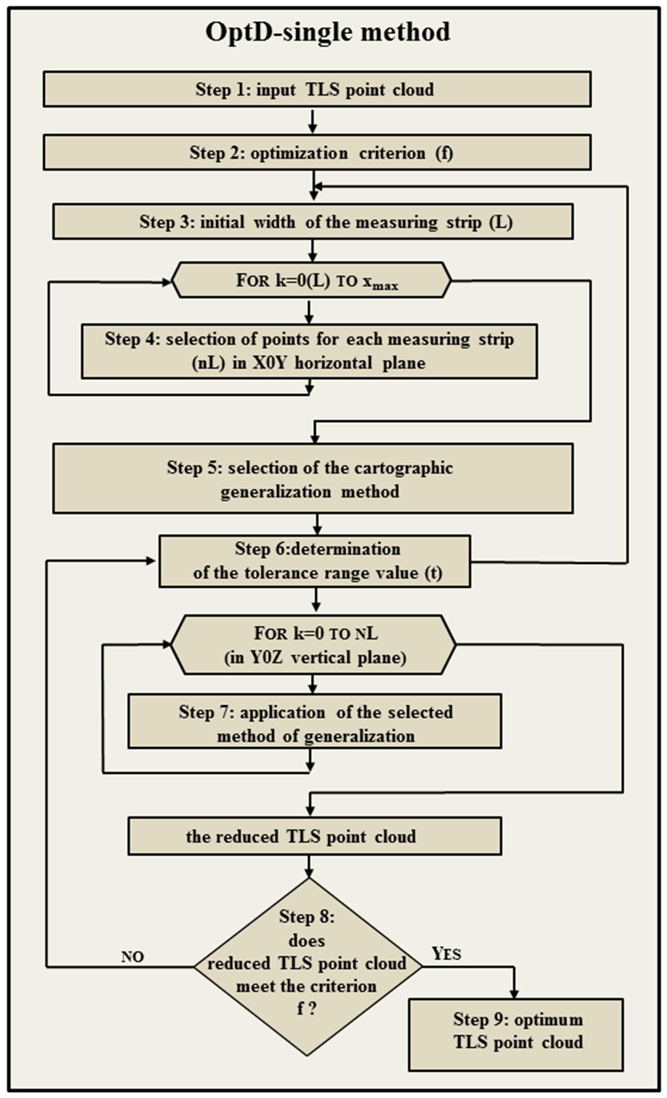
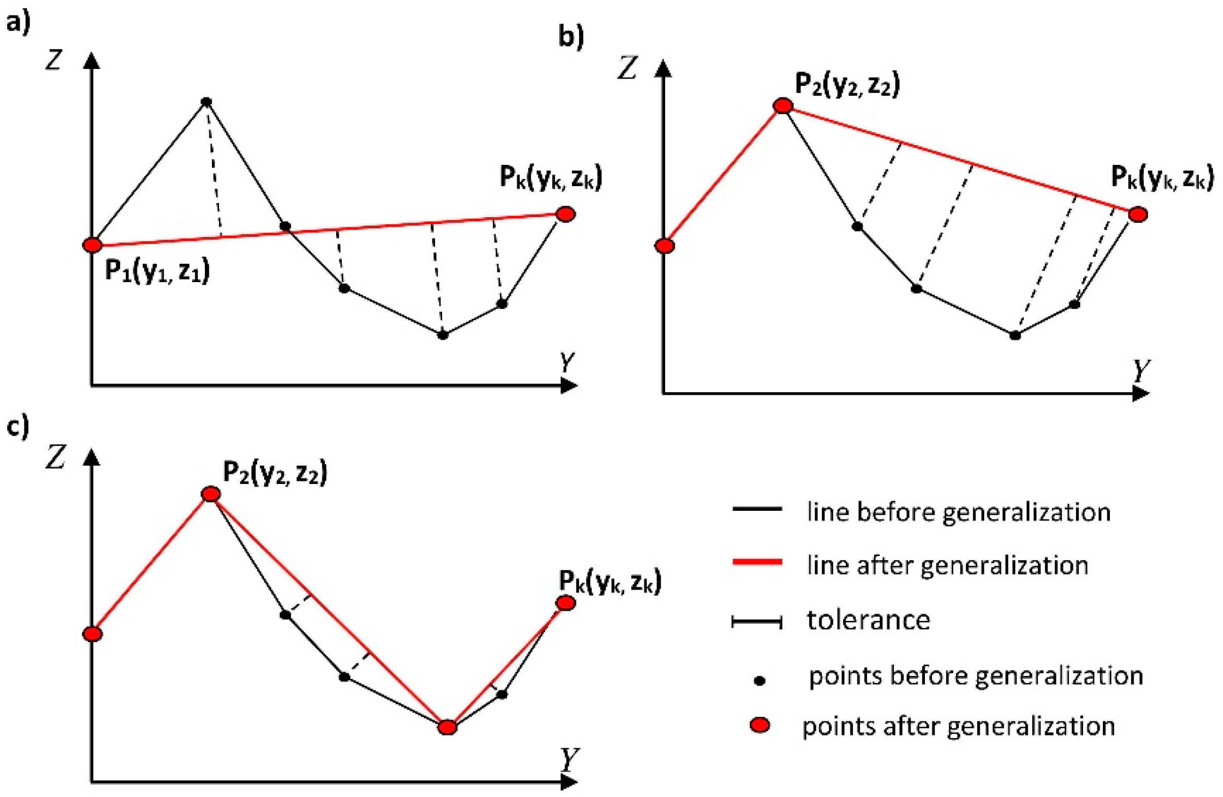
3. Optimization of Large Datasets Based on Using OptD Single Method

The OptD method is a reduction method that is fully automated and gives an optimal result due to the optimization criteria. The OptD method can be conducted in two ways:
Option 1: OptD method with single-objective optimization (OptD-single) [35];
Option 2: OptD method with multi-objective optimization (OptD-multi) [36].
These methods differ in the number of optimization criteria and the time needed to perform the reduction. Furthermore, several solutions can be obtained in the OptD-multi method. In this paper, we decided to use the OptD-single option. The number of points in datasets was important during processing, and therefore one criterion in the form of percentage points was used. The steps and scheme of this method were presented in detail in [36]. In that paper, the OptD-single method was tested on data from Airborne Laser Scanning (ALS). The results showed that, with the OptD-single method, the preparation of the data for DTM construction is less time-consuming. The time required for the implementation of the OptD method can be considered as negligible in the whole process of preparing the data for the DTM construction. For a file size of 682,344 KB (about 20 million points), the OptD method lasted for about 72 s (for 50% reduction) and 105 s (for 90% reduction) [37]. It allows for effective DTM generation and reducing the time and cost of LIDAR point cloud processing, which in turn enables the conduction of efficient analyses of acquired information resource.
The OptD method was developed in such a way that it takes into account different levels of reduction in the individual parts of the processing area. As a result, there are more points in detailed parts of the scanned object. In the case of uncomplicated structures or areas, the number of points is much smaller. Only those points that are significant will remain. A very important advantage of the method is the fact that during the processing the user has total control over the number of points in the dataset. Such advantages of the method can be very useful during the technical inspection of buildings, especially during the detection of defects and cracks.
The OptD method is a reduction method, which means that the real measurement points will remain in the dataset. This is important, since in the case of reducing the size of the dataset by the generation method, in the resulting dataset one obtains interpolated coordinates [38,39].
The OptD method uses linear object generalization methods, however the calculations are performed in a vertical plane, which allows the elevation component to be accurately controlled. The generalization approach used in the OptD method are the Douglas–Peucker [40], Visvalingam–Whyatt [41], and Opheim [42] methods.
During the operation of the method, the following parameters are selected: width of the measuring strip and tolerance used in the generalization method. The values of these parameters are calculated without user intervention and changed in the iterative process in such a way that the optimization criterion is met.
The assumption of using the OptD-single method was that reducing the dataset would not disturb the nature of the object, and, in particular, leaves more points in the cracks, crevices, and cavities. To this point, a methodology for the down-sampling of TLS data taking into account the OptD-single method was developed. The simplified diagram of the OptD-single methods is presented in Figure 1.
The OptD-single procedure has been used in original software, and proceeds in the following stages:
step 1: Input TLS data with cracks, crevices, and cavities.
step 2: Determination of the optimization criterion (f), here: percentage of points in dataset after reduction. This is the only step that requires input from the user.
step 3: Determination of the initial width of the measuring strip (L). The measuring strips are the narrow parts of the point cloud on the wall of building. The number of points that will be included in one strip depends on the width of the strip and scan density. Parameter L does not depend on the user, but rather, on optimization criterion. Successive values of the measuring strip are determined in the iterative process and are changed with a fixed interval. The division of the area covered by points into measurement strips (nL) in X0Y horizontal plane (in the wall coordinate system).
step 4: Selection of points for each measuring strip.
step 5: Selection of the cartographic generalization method, here: Douglas–Peucker (D-P) method. The scheme of the D-P method is presented in Figure 2.
step 6: Determination of the distance of tolerance range value (t) in the D-P method. The t value is determined in the iterative process and increases or decreases at every fixed interval.
step 7: Application of the selected method of generalization in the Y0Z vertical plane. Each measuring strip is processed separately. Points in the measuring strip are projected onto the Y0Z plane. In this way, a 2D image of the points is obtained and the line generalization method is possible. The result of the reduction in the example strip is presented in Figure 3. This is only a general example to show the algorithm operation.
step 8: Verification, whether obtained in the step 7 dataset, fits the specified criterion optimization. If so, the reduction process is completed, and the obtained dataset from step 7 is optimal. If not, steps 6–8 are repeated, wherein in step 6 the value of tolerance parameter is changed. If repeating steps 6–8 does not give a solution, go back to step 3 and change the width of the measuring strip.
step 9: Output the obtained result as an optimal dataset.
The algorithms of the OptD-single method were implemented in the Java programming language (v.9). The application was tested with both Oracle and OpenJDK runtime environment.

4. Materials and Experiments

4.1. Equipment

In this investigation, two types of terrestrial laser scanner system with different specifications were used. The first was a Leica ScanStation C10. This scanner is based on the time of flight principle, and its laser source emits visible impulses at a wavelength of 532 nm. The maximum instantaneous scan rate is up to 50,000 points per second. The laser spot size is equal to 4.5 mm for FWHH-based model (Full Width at Half Height) and 7 mm for Gaussian-based model for the range 0–50 m. The maximum measuring range is 300 m at 90% albedo and 134 m at 18% albedo, respectively. The second scanner used in this study was a Z+F IMAGER 5016. This scanner uses the phase-shift technique to achieve distance measurement. The maximum measurement range is 365 m. The maximum scan rate is up to 1.1 million points per second. The laser spot size is equal to 3.5 mm for Gaussian-based model and the laser beam divergence is equal to 0.3 mrad.

4.2. Data Acquisition

The research program covered experiments on two different samples. The first experiment was to scan a specially prepared concrete specimen with a crack (Figure 4). The crack width was approximately 5 mm. The measurement was made with the Leica ScanStation C10 impulse scanner from a distance of 10 m. During the research, the maximum scanning resolution was set. The second phase of the research program consisted of measurements of a real object—the Kościuszko Mound in Cracow, Poland. The location of the monument is the natural Blessed Bronisława Hill. A brick citadel around the Mound was built between 1850 and 1854. Currently, some parts of the citadel are characterized by poor technical condition (Figure 4). The Z+F IMAGER 5016 scanner was used for the second phase of the research. The measurement was made from a short distance of 7 m, and a super high resolution was set in the scanner.

4.3. Data Processing

The Leica Cyclone and Z+F Laser Control software were used for the pre-processing of data. The optimization of the dataset was carried out in original program implemented in the Java (v.9) programming language. The CloudCompare software was used to visualize and present the reduced dataset. The dataset from the TLS measurement of the concrete sample was processed in two ways. In the first approach, the OptD method was applied. The optimization criterion was the percentage of points left in the resulting dataset. Each reduced dataset was called “i dataset”, where i is the percentage of points that are left in the dataset after optimization. Ultimately, in addition to the original dataset, five reduced datasets were obtained (50%, 20%, 10%, 5%, and 2% datasets). In the second approach, the random way to reduce the dataset was applied. In the random way, the CloudCompare simply picks the specified number of points in a random manner [43]. Similarly, as in the case of the OptD method, a reduction was made to create five new datasets.
The purpose of analyzing TLS data from building diagnostic measurements is to identify defective parts in the building wall. For the automatic detection of defects on flat surfaces, the Mean Sum Error (MSE) method can be used [32]. The MSE method uses the distance of each point (di) from the reference plane (π) as the criterion to identify the cavities and cracks. In order to find an aforementioned optimal reference plane, the regression of three variables is used. Next, a predetermined tolerance value (ε) needs to be manually assigned for the research area. The tolerance value mainly depends on the tested object (object properties) and the used TLS (the scanner mechanism). Ultimately, the detection of defects on the flat surfaces is carried out by comparing the determined distance of each point with the tolerance value (di > ε).
In this research, the reference plane was determined based on the original dataset, i.e., the point cloud of the research area. The tolerance value ε for the concrete sample was taken as 5 mm. The data processing was performed separately for each dataset. The locations of cracks were determined by analyzing the distance (di > 5 mm). The results of the analysis for the OptD method and random method are presented in Figure 5 and Figure 6, respectively. The red colour indicates a separate dataset on the crack. The quantitative comparisons between the original and reduced point clouds are presented in Table 1 and Table 2.
The analyses of all datasets from the TLS measurement of the brick wall were carried out in the same way as for the concrete sample. The tolerance value ε for the brick wall was taken as 15 mm. The tolerance value ε increased in this case, as the brick wall fits the flat surface worse than a concrete element. Figure 7 and Figure 8 present images of the distribution of points for the OptD method and the random method, respectively. The red colour indicates a separate dataset on the damage area. Additionally, Table 3 and Table 4 summarize the number of points in each dataset and their percentage values.

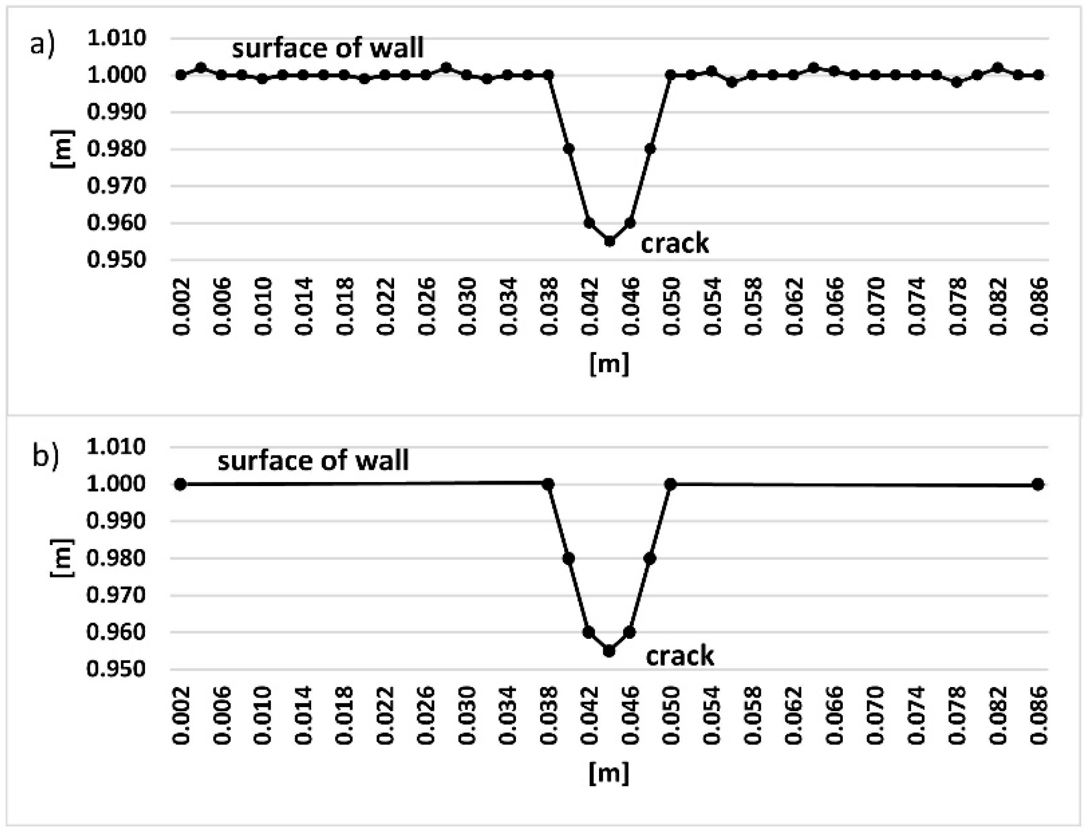
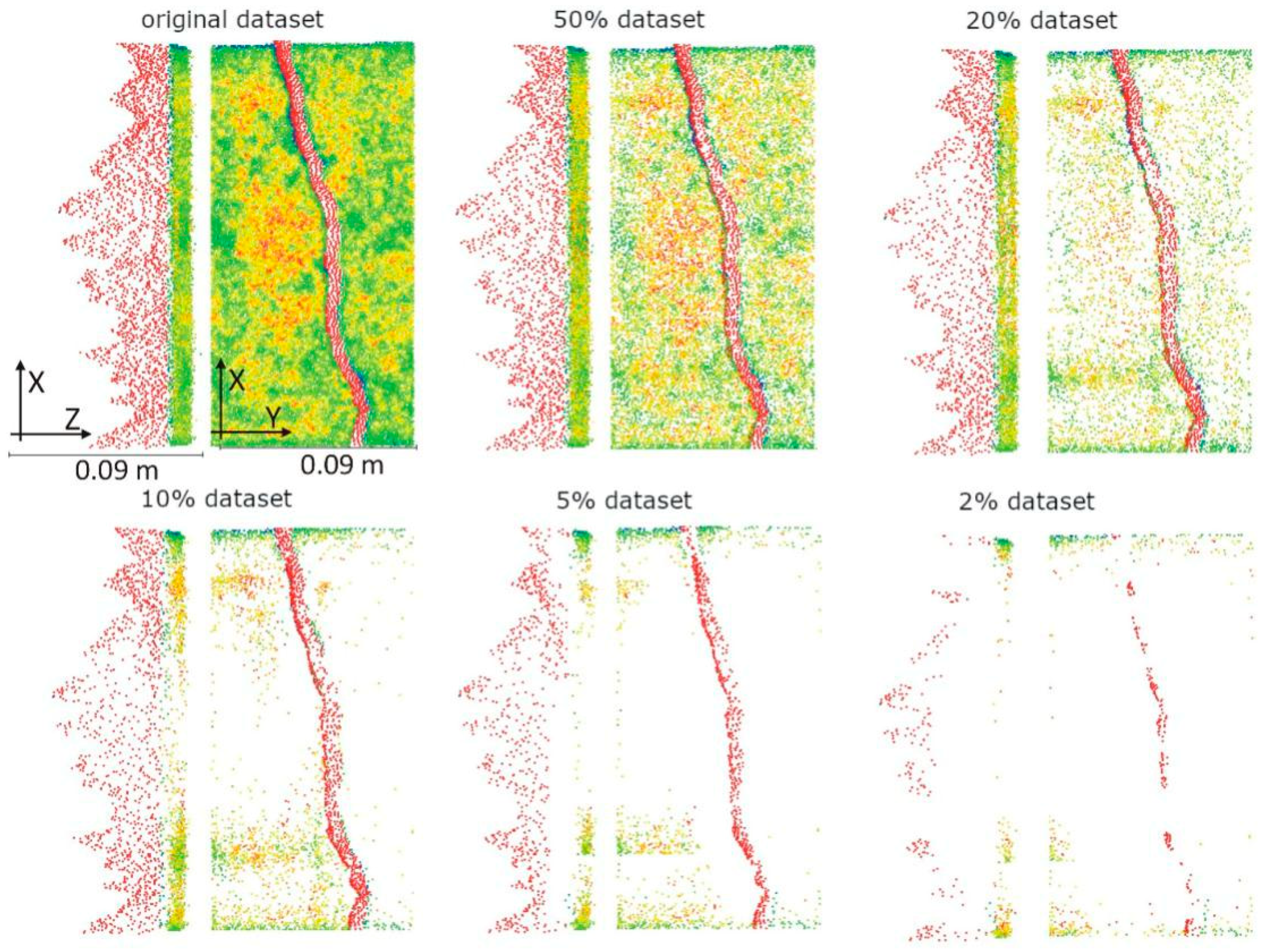
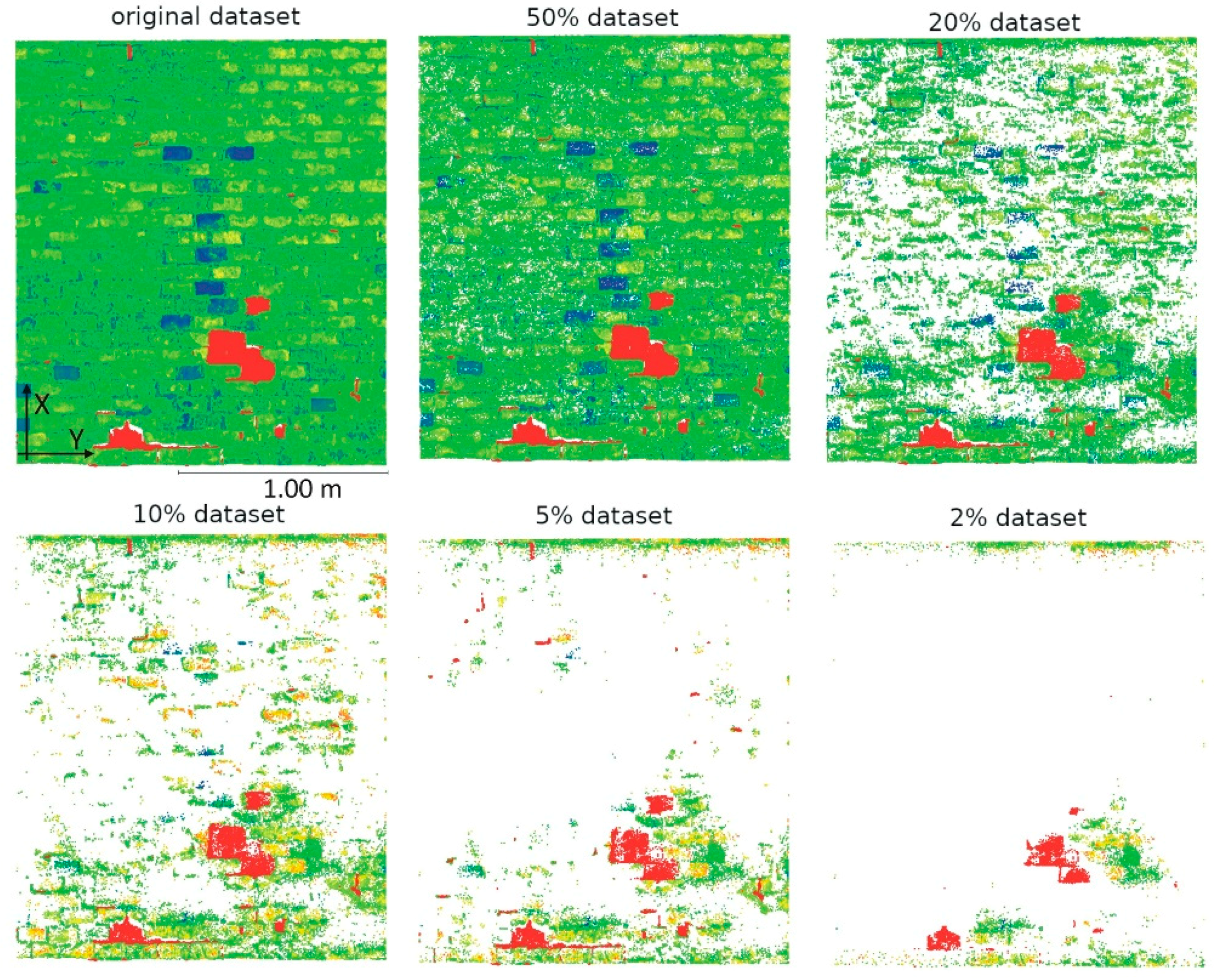
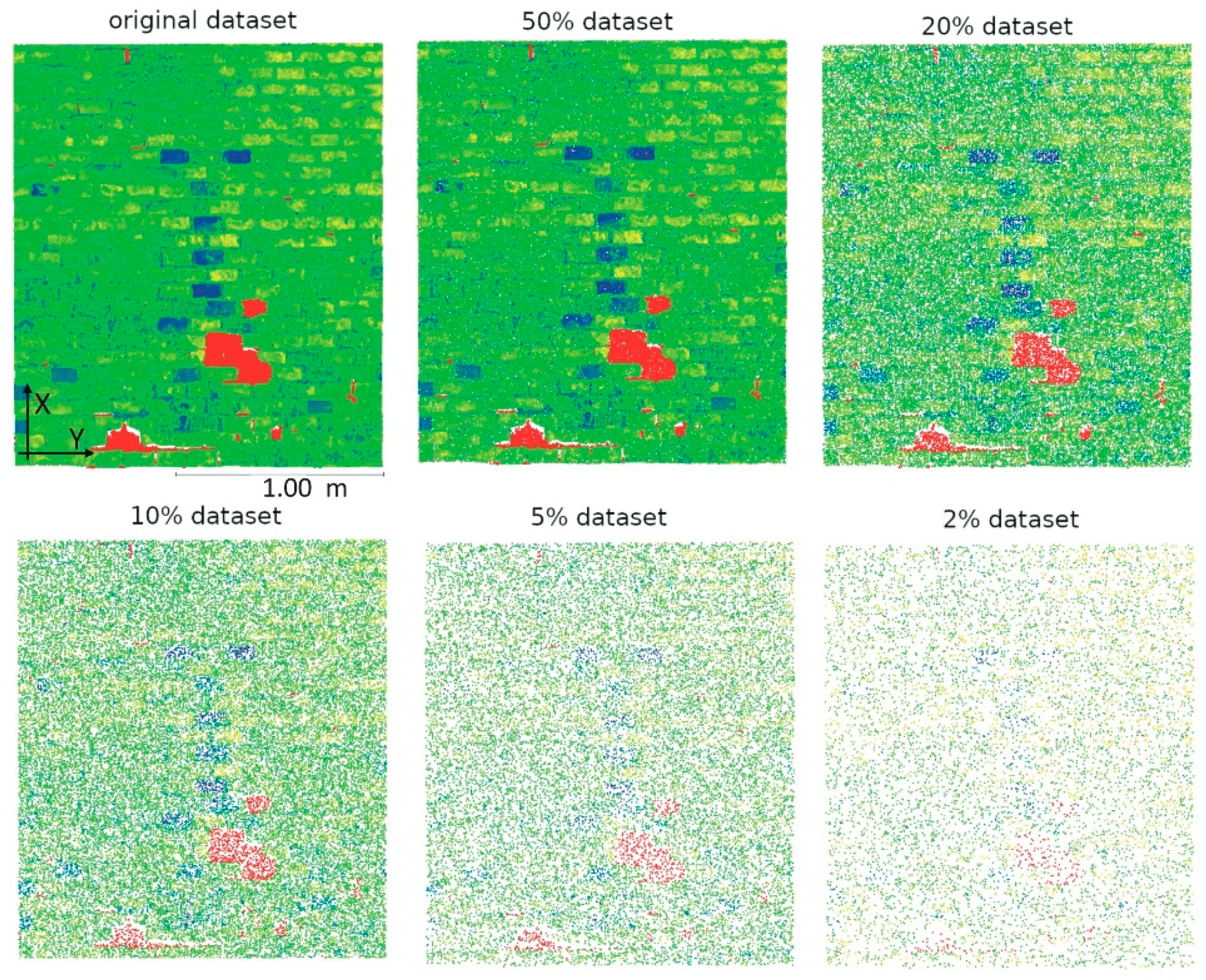
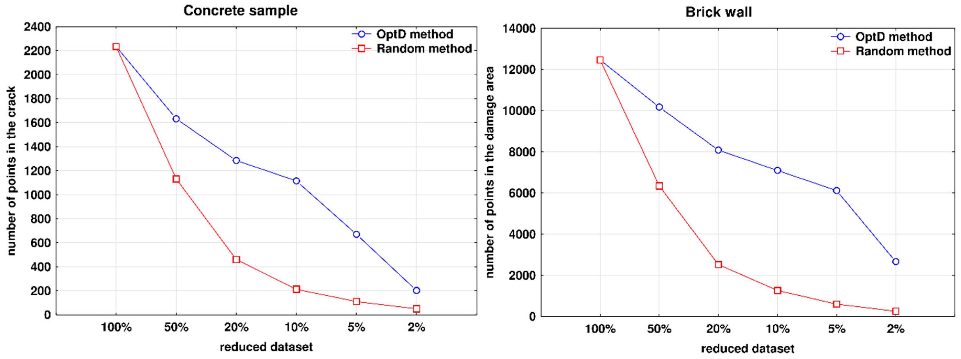
5. Results and Discussion

Usually, when the number of points in a dataset decreases evenly, then the details achieved from the data are significantly reduced. Thus, excessively low resolution of the point cloud does not allow the correct identification of wall damages (cavities and cracks). Such a situation can be seen in the reduction of data by the random method.
As shown in Figure 5, e.g., 10% regarding concrete sample reduction of the dataset by the OptD method, a significantly greater number of points are left in the recesses. In the case of reduction of the dataset by the random method, the dataset lost too many points in the crack to provide reliable interpretation of data (Figure 6). By visually evaluating the 10% dataset, it can be concluded that a reliable interpretation of the crack is possible. By comparing the results of two different reduced 10% dataset (Table 1 and Table 2), one can see the number of points on the crack. The OptD method preserved 1115 points, while the random method only preserved 212 points, i.e., approximately five times more points on the crack. For the 10% dataset (Table 1), only around 50% of the points on the crack were reduced. Therefore, the OptD method provides significant benefits for this case.
Similar to the previous example, the 10% reduced dataset on the brick wall was analyzed. By making a visual evaluation of this dataset (Figure 6 and Figure 7), it can be concluded that the OptD method left more points on the defects of wall than the random method. The obtained results, shown in Table 3 and Table 4, show the number of points that were left on the wall defects for the OptD method and random method, respectively. The OptD method preserved 7091 points, while the random method only preserved 1257 points. This is approximately five times more points on the wall defects. The difference for the 20% dataset is about three times more, and for the 5% dataset is about 10 times more. In the authors’ opinion, the 2% dataset was excessively reduced.
The overarching goal of the conducted research was to indicate the usefulness of the OptD method for the reduction of large datasets from TLS measurements of the technical condition of buildings and structures. The conducted research proved the benefits of using the OptD method to reduce point clouds. In the analyzed examples, the number of points on the defects for the OptD method is always significant greater than for the random method (see Figure 9). By comparing the values of the OptD method (blue line) and the values of the random method (red line), one can see the differences in the number of points related to the cracks and cavities for each reduced dataset.
Using the OptD method to reduce the dataset allows much better diagnostics of buildings and structures compared to the random method. It should be noted that the various software for processing point clouds do not have such an approach to reduce the datasets. Some software exists with reduction strategies based on different criteria, such as a curvature method, random method, space method, octree method (see software such as Leica Cyclone, CloudCompare, Z+F Laser Control, Geomagic Suite). The OptD method is fully automatic; the user only needs to specify the optimization criterion on the basis of point cloud resolution. Down-sampling of the OptD method allows different degrees of reduction declared by the user. The results show that more points remained where there were cracks and cavities, and less where there was a regular wall structure. Thanks to this, the process of automatic crack and defect detection can be improved. It should be noted that the effective crack detection on the building wall also depends on the type of scanner (PS or TOF) and its technical specifications, such as maximum scan resolution, laser spot size, laser beam divergence, and measurement noise. The measurement noise and so-called “edge effect” make data analysis difficult.

6. Conclusions

In this paper, the OptD method for the TLS point cloud down-sampling was proposed in the context of detecting defects in a building wall. Based on the conducted research, the following conclusions can be drawn:
  • The results prove that the proposed OptD method is appropriate for reducing the TLS dataset in the diagnostics of buildings and structures;
  • The down-sampling of the point clouds from the wall measurement using the OptD method allows more points to be left in the detailed part of the scanned object (crack or cavity) than in uncomplicated structures or areas (even surface);
  • The OptD method allows total control over the number of points in the dataset after reduction;
  • The disadvantage of the proposed OptD method is that it leaves a large number of points at the border research area.
Authors have been working to implement the OptD method in practical applications by implementing an algorithm in point cloud data processing software. By reducing the dataset with the OptD method, points are generally left on wall defects. Keeping this fact in mind, in the future the authors will complement the OptD method with automatic data segmentation. The modified OptD method will be used as a completely automatic method to detect defects on the walls of buildings related to cracks and cavities.

Author Contributions

Conceptualization, C.S.; Data curation, C.S. and W.B.-B.; Formal analysis, C.S.; Methodology, C.S.; Software, W.B.-B.; Visualization, W.B.-B.

Funding

The measurement with the Z+F IMAGER 5016 scanner was funded by Miniatura 1 (National Science Centre, Poland), grant number DEC-2017/01/X/ST10/01910.

Conflicts of Interest

The authors declare no conflicts of interest.

References

  1. Prantl, H.; Nicholson, L.; Sailer, R.; Hanzer, F.; Juen, I.; Rastner, P. Glacier Snowline Determination from Terrestrial Laser Scanning Intensity Data. Geosciences 2017, 7, 60. [Google Scholar] [CrossRef]
  2. Barbarella, M.; Fiani, M.; Lugli, A. Uncertainty in terrestrial laser scanner surveys of landslides. Remote Sens. 2017, 9, 113. [Google Scholar] [CrossRef]
  3. Suchocki, C. Application of terrestrial laser scanner in cliff shores monitoring. Rocz. Ochr. Sr. 2009, 11, 715–725. [Google Scholar]
  4. Janowski, A.; Szulwic, J.; Tysiąc, P.; Wojtowicz, A. Airborne And Mobile Laser Scanning In Measurements Of Sea Cliffs On The Southern Baltic. Photogramm. Remote Sens. 2015, 2015, 17–24. [Google Scholar] [CrossRef]
  5. Corso, J.; Roca, J.; Buill, F. Geometric Analysis on Stone Façades with Terrestrial Laser Scanner Technology. Geosciences 2017, 7, 103. [Google Scholar] [CrossRef]
  6. Ziolkowski, P.; Szulwic, J.; Miskiewicz, M. Deformation Analysis of a Composite Bridge during Proof Loading Using Point Cloud Processing. Sensors 2018, 18, 4332. [Google Scholar] [CrossRef] [PubMed]
  7. Cabaleiro, M.; Riveiro, B.; Arias, P.; Caamaño, J.C. Algorithm for beam deformation modeling from LiDAR data. Meas. J. Int. Meas. Confed. 2015, 20–31. [Google Scholar] [CrossRef]
  8. Riveiro, B.; González-Jorge, H.; Varela, M.; Jauregui, D.V. Validation of terrestrial laser scanning and photogrammetry techniques for the measurement of vertical underclearance and beam geometry in structural inspection of bridges. Meas. J. Int. Meas. Confed. 2013, 784–794. [Google Scholar] [CrossRef]
  9. Suchocki, C.; Katzer, J. TLS technology in brick walls inspection. In Proceedings of the 2018 Baltic Geodetic Congress (BGC Geomatics), Olsztyn, Poland, 21–23 June 2018; IEEE: Olsztyn, Poland, 2018; pp. 359–363. [Google Scholar]
  10. Suchocki, C.; Jagoda, M.; Obuchovski, R.; Šlikas, D.; Sužiedelytė-Visockienė, J. The properties of terrestrial laser system intensity in measurements of technical conditions of architectural structures. Metrol. Meas. Syst. 2018, 25, 779–792. [Google Scholar] [CrossRef]
  11. Bobkowska, K.; Szulwic, J.; Tysiąc, P. Bus bays inventory using a terrestrial laser scanning system. MATEC Web Conf. 2017, 122, 1–6. [Google Scholar] [CrossRef]
  12. Tan, K.; Cheng, X.; Ju, Q.; Wu, S. Correction of Mobile TLS Intensity Data for Water Leakage Spots Detection in Metro Tunnels. IEEE Geosci. Remote Sens. Lett. 2016, 13, 1711–1715. [Google Scholar] [CrossRef]
  13. Rodríguez-Gonzálvez, P.; Fernández-Palacios, B.J.; Muñoz-Nieto, Á.L.; Arias-Sanchez, P.; Gonzalez-Aguilera, D. Mobile LiDAR system: New possibilities for the documentation and dissemination of large cultural heritage sites. Remote Sens. 2017, 9, 189. [Google Scholar] [CrossRef]
  14. Rüther, H.; Chazan, M.; Schroeder, R.; Neeser, R.; Held, C.; Walker, S.J.; Matmon, A.; Horwitz, L.K. Laser scanning for conservation and research of African cultural heritage sites: The case study of Wonderwerk Cave, South Africa. J. Archaeol. Sci. 2009, 36, 1847–1856. [Google Scholar] [CrossRef]
  15. Chiabrando, F.; Lo Turco, M.; Rinaudo, F. Modeling the decay in an hbim starting from 3d point clouds. A followed approach for cultural heritage knowledge. In Proceedings of the 26th International CIPA Symposium 2017, Ottawa, ON, Canada, 28 August–1 September 2017; pp. 605–612. [Google Scholar] [CrossRef]
  16. Liu, W.; Chen, S.; Hauser, E. LiDAR-based bridge structure defect detection. Exp. Tech. 2011, 35, 27–34. [Google Scholar] [CrossRef]
  17. Bian, H.; Bai, L.; Chen, S.-E.; Wang, S.-G. Lidar Based Edge-Detection for Bridge Defect Identification. In Proceedings of the SPIE Smart Structures and Materials + Nondestructive Evaluation and Health Monitoring, San Diego, CA, USA, 11–15 March 2012. [Google Scholar] [CrossRef]
  18. Suchocki, C.; Katzer, J.; Rapiński, J. Terrestrial Laser Scanner as a Tool for Assessment of Saturation and Moisture Movement in Building Materials. Period. Polytech. Civ. Eng. 2018, 62, 1–6. [Google Scholar] [CrossRef]
  19. Suchocki, C.; Katzer, J. Terrestrial laser scanning harnessed for moisture detection in building materials—Problems and limitations. Autom. Constr. 2018, 94, 127–134. [Google Scholar] [CrossRef]
  20. Teza, G.; Galgaro, A.; Moro, F. Contactless recognition of concrete surface damage from laser scanning and curvature computation. NDT E Int. 2009, 42, 240–249. [Google Scholar] [CrossRef]
  21. Riveiro, B.; Morer, P.; Arias, P.; De Arteaga, I. Terrestrial laser scanning and limit analysis of masonry arch bridges. Constr. Build. Mater. 2011, 25, 1726–1735. [Google Scholar] [CrossRef]
  22. Kedzierski, M.; Fryskowska, A. Methods of laser scanning point clouds integration in precise 3D building modelling. Meas. J. Int. Meas. Confed. 2015, 221–232. [Google Scholar] [CrossRef]
  23. Armesto-González, J.; Riveiro-Rodríguez, B.; González-Aguilera, D.; Rivas-Brea, M.T. Terrestrial laser scanning intensity data applied to damage detection for historical buildings. J. Archaeol. Sci. 2010, 37, 3037–3047. [Google Scholar] [CrossRef]
  24. Laefer, D.F.; Truong-Hong, L.; Carr, H.; Singh, M. Crack detection limits in unit based masonry with terrestrial laser scanning. NDT E Int. 2014, 62, 66–76. [Google Scholar] [CrossRef] [Green Version]
  25. Du, X.; Zhuo, Y. A point cloud data reduction method based on curvature. In Proceedings of the 2009 IEEE 10th International Conference on Computer-Aided Industrial Design and Conceptual Design: E-Business, Creative Design, Manufacturing—CAID CD’2009, Wenzhou, China, 26–29 November 2009; pp. 914–918. [Google Scholar] [CrossRef]
  26. Mancini, F.; Castagnetti, C.; Rossi, P.; Dubbini, M.; Fazio, N.L.; Perrotti, M.; Lollino, P. An integrated procedure to assess the stability of coastal rocky cliffs: From UAV close-range photogrammetry to geomechanical finite element modeling. Remote Sens. 2017, 9, 1235. [Google Scholar] [CrossRef]
  27. Orts-Escolano, S.; Morell, V.; Garcia-Rodriguez, J.; Cazorla, M. Point cloud data filtering and downsampling using growing neural gas. In Proceedings of the International Joint Conference on Neural Networks, Dallas, TX, USA, 4–9 August 2013. [Google Scholar] [CrossRef]
  28. Moreno, C.; Li, M. A comparative study of filtering methods for point clouds in real-time video streaming. In Lecture Notes in Engineering and Computer Science, Proceedings of the World Congress on Engineering and Computer Science 2016, San Francisco, USA, 19–21 October 2016; Newswood Limited: Hong Kong, China, 2016; ISBN 978-988-14047-1-8. [Google Scholar]
  29. Jang, J.; Hwang, S.; Park, K. Intensity control of a phase-shift based laser scanner for reducing distance errors caused by different surface reflectivity. In Proceedings of the International Conference on Sensing Technology ICST, Palmerston North, New Zealand, 28 November–1 December 2011. [Google Scholar] [CrossRef]
  30. San José Alonso, J.I.; Martínez Rubio, J.; Fernández Martín, J.J.; García Fernández, J. Comparing Time-of-Flight and Phase-Shift. the Survey of the Royal Pantheon in the Basilica of San Isidoro (León). ISPRS Int. Arch. Photogramm. Remote Sens. Spat. Inf. Sci. 2012, XXXVIII-5/W16, 377–385. [Google Scholar] [CrossRef]
  31. Jacobs, G. Understanding Spot Size for Laser Scanning. Professional Surveyor Magazine, October 2006. [Google Scholar]
  32. Crespo, C.; Armesto, J.; González-Aguilera, D.; Arias, P. Damage Detection on Historical Buildings Using Unsupervised Classification Techniques. Int. Arch. Photogramm. Remote Sens. Spat. Inf. Sci. 2010, XXXVIII, 184–188. [Google Scholar]
  33. Rabah, M.; Elhattab, A.; Fayad, A. Automatic concrete cracks detection and mapping of terrestrial laser scan data. NRIAG J. Astron. Geophys. 2013, 250–255. [Google Scholar] [CrossRef]
  34. Lin, Y.-J.; Benziger, R.R.; Habib, A. Planar-Based Adaptive Down-Sampling of Point Clouds. Photogramm. Eng. Remote Sens. 2016, 82, 955–966. [Google Scholar] [CrossRef]
  35. Błaszczak-Bąk, W.; Sobieraj-Żłobińska, A.; Kowalik, M. The OptD-multi method in LiDAR processing. Meas. Sci. Technol. 2017, 28, 7500–7509. [Google Scholar] [CrossRef]
  36. Błaszczak-Bąk, W. New optimum dataset method in LiDAR processing. Acta Geodyn. Geomater. 2016, 13, 381–388. [Google Scholar] [CrossRef]
  37. Błaszczak-Bąk, W.; Koppanyi, Z.; Toth, C. Reduction Method for Mobile Laser Scanning Data. ISPRS Int. J. Geo-Inf. 2018, 7, 285. [Google Scholar] [CrossRef]
  38. Bauer-Marschallinger, B.; Sabel, D.; Wagner, W. Optimisation of global grids for high-resolution remote sensing data. Comput. Geosci. 2014, 72, 84–93. [Google Scholar] [CrossRef]
  39. Gosciewski, D. Selection of interpolation parameters depending on the location of measurement points. GIScience Remote Sens. 2013, 50, 515–526. [Google Scholar] [CrossRef]
  40. Douglas, D.H.; Peucker, T.K. Algorithms for the reduction of the number of points required to represent a digitized line or its caricature. Can. Cartogr. 1973, 10, 112–122. [Google Scholar] [CrossRef]
  41. Visvalingam, M.; Whyatt, J.D. Line generalisation by repeated elimination of points. Cartogr. J. 1993, 30, 46–51. [Google Scholar] [CrossRef]
  42. Opheim, H. Smoothing a digitized curve by data reduction methods. In Eurographics Conference Proceedings; Encarnacao, J.L., Ed.; The Eurographics Association: Munich, Germany, 1981; pp. 127–135. [Google Scholar]
  43. CloudCompare User Manual, Version 2.6.1. 2018. Available online: www.cloudcompare.org (accessed on 5 January 2019).
Figure 1. The simplified diagram of the OptD-single methods.
Geosciences 09 00070 g001
Figure 2. Principle of operation of the Douglas–Peucker (D-P) method (source: study based on Douglas and Peucker (1973) [40]).
Geosciences 09 00070 g002
Figure 3. Results of the reduction process in measuring strip (a) before reduction, (b) after reduction.
Geosciences 09 00070 g003
Figure 4. The research objects: concrete sample (on the left) and brick wall of the citadel (on the right).
Geosciences 09 00070 g004
Figure 5. Damage mapping results in a concrete sample using the OptD method.
Geosciences 09 00070 g005
Figure 6. Damage mapping results in a concrete sample using the random method.
Geosciences 09 00070 g006
Figure 7. Damage mapping results in a brick wall using the OptD method.
Geosciences 09 00070 g007
Figure 8. Damage mapping results in a brick wall using the random method.
Geosciences 09 00070 g008
Figure 9. Reduction of points on the crack and cavities using the OptD method and the random method.
Geosciences 09 00070 g009
Table 1. Results of processing with the OptD method—concrete sample.
Total Number of PointsNo Damage (di ≤ 5 mm)Damage (di > 5 mm)
Number of Points% Original DatasetRelation to the Original DatasetNumber of Points% Original DatasetRelation to the Original Dataset
original dataset329383070493.2100%22346.8100%
50% dataset163521472090.047.9%163210.073.1%
20% dataset6594531080.517.3%128419.557.5%
10% dataset3316220166.47.2%111533.649.9%
5% dataset165398359.53.2%67040.530.0%
2% dataset65945669.21.5%20330.89.1%
Table 2. Results of processing with the random method—concrete sample.
Total Number of PointsNo Damage (di ≤ 5 mm)Damage (di > 5 mm)
Number of Points% Original DatasetRelation to the Original DatasetNumber of Points% Original DatasetRelation to the Original Dataset
original dataset329383070493.2100%22346.8100%
50% dataset163521522193.149.6%11316.950.6%
20% dataset6594613493.020.0%4607.020.6%
10% dataset3316310493.610.1%2126.49.5%
5% dataset1653154393.35.0%1106.74.9%
2% dataset65961092.62.0%497.42.2%
Table 3. Results of processing with the OptD method—brick wall.
Total Number of PointsNo Damage (di ≤ 15 mm)Damage (di > 15 mm)
Number of Points% Original DatasetRelation to the Original DatasetNumber of Points% Original DatasetRelation to the Original Dataset
original dataset45655644409697.3100%124602.7100%
50% dataset22916721899995.649.3%101684.481.6%
20% dataset915148343491.218.8%80808.864.8%
10% dataset455693847884.48.7%709115.656.9%
5% dataset226611654773.03.7%611427.049.1%
2% dataset9182652071.01.5%266229.021.4%
Table 4. Results of processing with the random method—brick wall.
Total Number of PointsNo Damage (di ≤ 15 mm)Damage (di > 15 mm)
Number of Points% Original DatasetRelation to the Original DatasetNumber of Points% Original DatasetRelation to the Original Dataset
original dataset45655644409697.3100%124602.7100%
50% dataset22916722282797.250.2%63402.850.9%
20% dataset915148899797.220.0%25172.820.2%
10% dataset455694431297.210.0%12572.810.1%
5% dataset226612206397.45.0%5982.64.8%
2% dataset9182893397.32.0%2492.72.0%

