Abstract
Real estate management, including real estate market analysis, is part of a so-called geosystem. In recent years, the popularity of creating various types of systems and automatic solutions in real estate management, including those related to property classification and valuation, has been growing in the world, mainly to reduce the impact of human subjectivity, to increase the scope of analyses and reduce research time. A very important fact that should be underlined is that properties are strongly related to geolocation (space) and strongly determine it. Authors proposed in the paper solutions that highlight implementation of geoscience and “geo-approach” combined with fuzzy logic methods that allow to decrease subjectivity in property analyses and diminish uncertainty in decision making process. The proposed methodology involves three main problematic components of decision support system in property investment analyses development with the use of geo-technologies such as: determination of the database model; elaboration geo-property-zones with geoprocessing activities; identification of homogeneous group of properties transactions. The influence of spatial decision factor determined in the study lead to objective and precise calculation of value differentiation from 22 to 43% depending on the property’s remoteness to the sea.
1. Introduction
Real estate is a part of the system that, in general, can be called a real estate market. The main problem in the analyses of the property market is the specific character of the information describing it. Decision making in relation to real estate is subject to great uncertainty and is very complex. Reducing the risk of making wrong decisions thus reducing uncertainty, can be done by precise specification of goal that is to be achieved and methods that are adapted to the specific circumstances of the analysed phenomenon [1].
Although it has recently become popular to create various types of support systems, there is still a lack of comprehensive and effective information systems for land management and real estate market analysis, especially considering their strict connotation with geolocation [2]. Spatial management and real estate market are kinds of systems that are parts of the general geosystem. Essentially, a geosystem is a structure that consolidates natural (in terms of spatial features), technical and social relations. According to Źróbek and Grzesik [3], the ability of synthetical perception of real estate as an object in a spatial context is important for correct planning decisions in space and investment management. Nowadays database engines are mostly based on the relations database model [4]. It should be emphasized that there is a very high risk of “scientific falsification” in which attempts are made to adapt reality to analytical methods, not as it should be (in accordance with the idea of scientific positivism [5,6]), an advisable selection of the method for the analysed empirical phenomena.
One of the most popular systems used currently in property analyses are Automated Valuation Models (AVMs). Particularly noteworthy is the fact that AVMs most often take into account the advantages given by geospatial connotation (association) of the properties (e.g., References [7,8,9]) that constitute structure within computer-assisted quantitative methods dedicated to support decision on property market.
This paper aims to analyse and solve the three problematic aspects of development decision support systems: determination of the database model; geo-property-zones elaboration with geoprocessing activities; identification of homogeneous group of properties transactions. The mentioned aspects are the crucial components of the real estate market support decision system with the use of geo-technologies that enable identification of influence of geolocation on property assessment. The original value of the paper constitutes proposal of new decision-making support systems engineering. Particularly elaborations within it and development of applications that enable control of obtained results.
2. Literature Review and Research Issues
The properties are strongly related to geolocation (space) and strongly determine it. In the classical approach, geolocation is understood as the location and process of determining the geographical location of objects and is closely related to the so-called positioning. Geolocation of real estate or real estate market has a wider meaning as an assumption adopted in the study. It is assumed that geolocation of the real estate market in terms of real estate valuation is considered not only in relation to the classic reference to the land surface but also in the context of an additional dimension not directly related to the location on Earth but to existence of determinants of properties value such as, for example, local zoning, lot size, topography or even flood risk [10,11]. The additional dimension is associated with the classification of urban space and the real estate itself on the basis of diverse spatial, anthropogenic, natural, social, economic, political or behavioural factors [8]. In this approach, factors influencing the value of real estate constitute a kind of geoinformation included in a multidimensional information system.
The necessity of determining structural and spatial similarities of property markets results from various needs related to the context of becoming acquainted with and analysing market mechanisms [2,3]. Each real estate market is locked in a specific, unique space. On the one hand, the specificity of real estate markets and real estate alone creates numerous opportunities in the area of creating various types of decision support systems, on the other hand it creates challenges for researchers due to the specificity of information concerning the properties. The specific character of information defining real estate market and properties is linked with the availability and imprecision of property information, the sudden and unpredictable changes, that often occur regarding analyses of properties and their location [12].
It should be clearly emphasized that the specificity of information about real estate causes that these variables are difficult to quantify, discretize and implement in the processes of analytical and numerical modelling. That’s why the developed system for gathering market data should be flexible and scalable enough to enable frequent modifications taking into account the specificity of property information. One of the most interesting solutions that support decision making on the property markets are automated valuation models (AVMs) that are popular in recent years on the one hand and controversial on the other.
Automated valuation models, defined as computer–assisted quantitative methods, can be applied in numerous aspects in property investment analyses. AVMs have their origins in North America, the first commercial application was created in 1981 and began to be developed in the UK in the 1990s. After the crisis in 2008 caused by the insolvency of mortgages, Robinson & Dawnie [13] demonstrated the growing importance of AVMs all over the world. In 2009, the European Mortgage Federation stressed that: ‘AVM is a useful and efficient tool when used appropriately by an experienced operator.’ The definition of integration between automated valuation and valuation in person was provided by the RICS in 2012 [14] and is as follows: ‘output from an AVM can be utilized as part of evidence in support of a valuation.’ The most popular method used in case of AVM technics is multiple regression analysis (MRA) that have several problems (among others): presence of excessive multicollinearity among attributes, spatial autocorrelation among residuals, diminishing the stability of regression coefficients [15,16,17,18,19,20]. According to the mentioned authors popular analytical method are relatively ineffective in weak-form efficient real estate markets. The fact of understanding and accepting the existence of an element of uncertainty in all areas of human life and acknowledging randomness, led to the development of theories based on stochastic laws of nature [21]. According to this theory, making decisions related to real estate in conditions of certainty, by definition, does not exist. One of the most important components that provides some stability (less uncertainty) is the support of analyses on geolocation [22,23]. Several researchers tried to compare different AVM techniques and methods including geo-solutions. Multiple Regression Analysis (MRA) were compared with the Spatial Autoregressive Model (SAM) by Borst & McCluskey [24] and the Spatial Extension Method by Wilhelmsson [25], indicating an improvement in the accuracy of MRA by the implementation of the SAM. Borst & McCluskey [26] compared Geographic Weighted Regression and the Comparable Sales Method. In this case, the Spatial Lag Model is found to improve MRA in terms of spatial autocorrelation. The spatial lag model was used by Quintos [27] to create location adjustment factors in order to include this in traditional Ordinary Least Squares (OLS). However, other researchers [28,29,30] underlined that, despite the enormous number of applications, statistic data analyses have theoretical weaknesses and may not be efficient in those markets where uncertainty is high due to the unavailability of information. For this reason, many authors tested alternative approaches to automated valuation. One of them considers the application of Neural Networks (NN) [31,32,33]. O’Connor [34] proposed efficient hybrid model structure and GIS location adjustments for AVM, whereas in a more detailed context Demetriou [35] GIS-based hedonic modelling in land consolidation schemes and Jozaghi et al. [2] applied Analytic Hierarchy Process (AHP) and Technique for Order of Preference by Similarity to Ideal Solution (TOPSIS) with GIS use for a spatial hydro-infrastructure problems solution. A different approach is represented by the use of the Rough Set Theory (RST) based on discrete mathematics. RST may be applied with little data without a causal mathematical relationship. The use of RST following the methodological improvement of the original assumptions was proposed by d’Amato [36], Aurelio & Gonzalez [37], Kauko & d’Amato [38], Renigier-Biłozor et al. [12,15] as the foundation of AVMs. The model estimated value based on the if–then rule instead of a continuous mathematical function.
3. Materials and Methods
3.1. Methodology of the Analyses and Scope of Data Analysis
The methodology assumed analyses in three main problematic aspects of the decision support system in property investment analyses development with the use of geo-technologies. Three mainstream aspects of the analyses are as follow:
- ➢
- determination of the database model—designation of attributes—gathering, developing and processing the descriptions/attributes of property transactions; the main elements of the database are as follow:
- -
- defining and coding technical attributes from public register of property transactions,
- -
- defining and coding geolocation attributes with the use of geocoding tools (for transforming a physical address description to a location on the Earth’s surface) Nominatim (see Section 4.3) for particular coordinate system, calculation Euclidean distance or routing distance along the public roads obtained as a vector data from Open Street Map (OSM) system, getting number of POI (specific point location interesting or useful for someone) in buffer zones,
- -
- defining and coding spatial decision factor—seashore of Baltic sea in this case—with the use of geotechnologies based on grid distance, fuzzy logic, rough set method.
- ➢
- geo–property–zones elaboration with geoprocessing activities:
- -
- designation of square grid,
- -
- elaboration of the buffer zones,
- -
- collection of geolocation attributes,
- -
- development of areas with the same characteristics (for all attributes separately).
- ➢
- identification of homogeneous group of property transactions—polarization of properties:
- -
- grouping/classifying the properties that are located in the zone relative to a significant decision factor in the space—that may define real estate market from geolocation point of view (e.g., costal property market),
- -
- grouping/classifying the properties regarding physical characteristics,
- -
- grouping/classifying the properties regarding attractiveness of the geolocation.
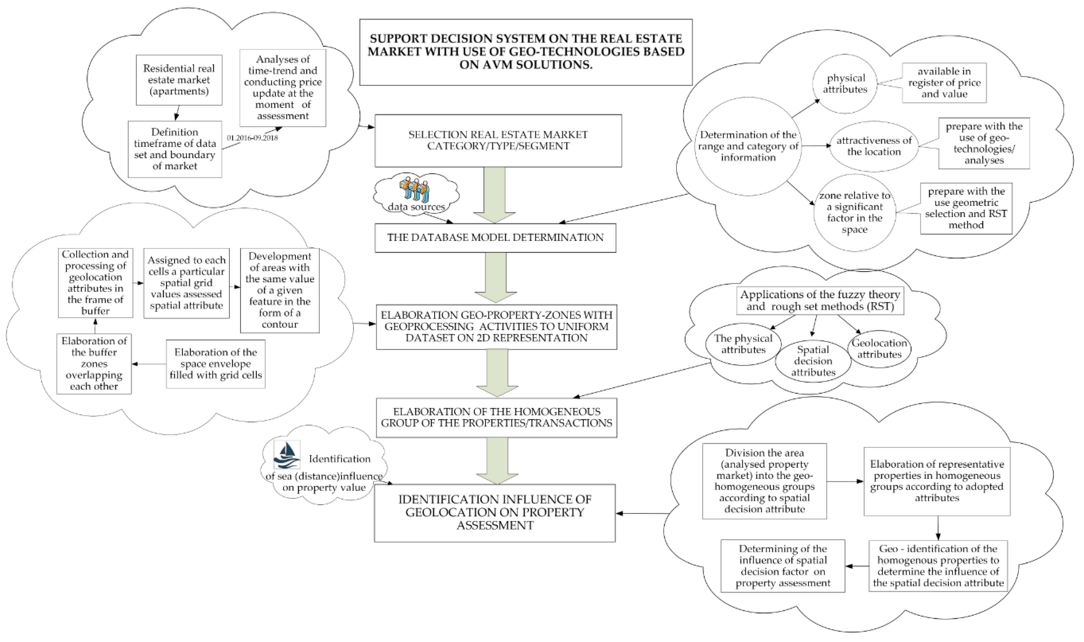
The presented aspects in transaction analyses constitute the worldwide debate on accuracy decrease and reliability of the obtained results regarding property market analyses. The authors present solutions that highlight implementation of geoscience and “geo–approach” methods that allow to solve or decrease subjectivity in property analyses. The authors of the article assumed high scalability and independence of the tested system. Georeferencing based on OSM collections located within the own database was used. The solution not only eliminated the necessity of external servers use but also decreased amount of time needed to acquire (via the Internet) mass spatial information and costs connected with it. Availability of spatial SQL solutions for leading database engine providers enabled the preparation of the system based on specific tools, according to universal assumptions today. The main aspects of the analysis were described in Figure 1.
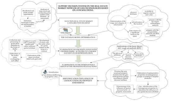
Figure 1.
Algorithm of decision system on the real estate market support with use of geo-technologies based on Automated Valuation Model (AVM) solutions on the example property transactions located in Gdynia (Poland)—coastal area. Source: Own elaboration.
The Figure 1 presents decision support system that consists of three main significant components: determination of the pattern of the database structure, elaboration zones with geoprocessing, identification of homogeneous group of properties. These components lead to identification influence of geolocation on property assessment as one of the main original aspects of the study. The proposed components can be considered as a separate procedure or can be approached either in the linear or simultaneous use. In this case the proposed components are in the synergy of the given system aimed at achieving a structured algorithm of decision support system on the real estate market. The algorithm was described in detail in the next chapter based on the empirical example.
3.2. Data Description
The study was conducted on the basis of dataset with date stamp reference from 1 January 2016 to 4 September 2018. The data included 2364 transactions of residential properties (apartments) that took place in Gdynia (Poland). The city has a mature and developed market with a sufficient number of transactions and a high demand and supply ratio. Gdynia is the developing city in very good economic condition perspective. The coastal city belongs to the so called Tricity (Gdańsk, Gdynia, Sopot) metropole located nearby the Baltic sea. Gdynia has a significant increase development in the frame of: economy, infrastructure, human capital, the functioning of public institutions, image and investment [39].
4. Empirical Results Based on Algorithm of Decision Support System for Property Analyses with the Use of Geo-Technology
4.1. Selection of Real Estate Market Category/Type/Segment
The very first step in the decision support algorithm involved selection of real estate market category/type/segment that in this case was the residential apartment market. Simultaneously, the timeframe of the dataset and the boundary of market had to be defined. In this case, the maritime Gdynia market and property transactions within the last 2.5 years (from 1 January 2016 to 4 September 2018) have been chosen. The transactions, in order to be comparable, should be brought forward to one moment of time. In this case designation of the time trend and coefficient changing prices in time had to be determined. The authors use regression modelling to designate the coefficient of changing prices per day. From regression analyses indicated that the unit prices change 1.65 PLN per day. Regarding maximum day differences between time of transactions that was 987 days indicated that the maximum changes is 1628 PLN per SQM. The results were confirmed by the National Polish Bank analyses that indicated the average prices changing between I quarter 2016 and III quarter 2018 were 1766 PLN on average. The prices were updated at the moment of assessment—1 October 2018 with the use of following formula:
where: —unit price of corrected transaction for time, —unit transaction price; —coefficient from linear regression analyses that present changing of unit price per day, —days differences between time of assessment and time of transaction.
4.2. Determination of the Pattern of the Database Structure
The next step in the procedure included determination of the database model structure of transaction in ordinary 1D spatial (point) representation. The first issue in this step assumed definition of the range and category of information. The following category and range of information was determined:
- -
- physical attributes—derived from public transactions register of price and value: usable area, location on the floor, number of rooms, building age, building materials,
- -
- attractiveness of location—prepared with the use of geo–analyses products: traffic noise, railway noise, distance from green areas, occurrence suburban train, occurrence shops, distance from points of early childhood education, occurrence of universities, occurrence public transport stops,
- -
- spatial decision factor—remoteness from the sea.
Verification of the available sources of information was conducted in the same stage. On the basis of literature analysis [12,40,41,42,43,44,45,46,47] and confrontation with an available source of property registry information the defining and coding of attributes was elaborated. The attribute domains for residential transactions were defined according to the criteria that are presented in Table 1.

Table 1.
Physical and geolocation attributes in property database.
4.3. Geo-Property-Zones Elaboration with Geoprocessing Activities
The next step assumed geo-property-zones elaboration with geoprocessing activities to transform dataset on 2D spatial (area-polygons) representation. The sets of numerical data related to the real estate market are characterized by a large volume, a large polarization of source, formats, methods of storage and access to them. These constitute difficulties of combining information relating to analysed transactions. Other source for difficulties involves:
- -
- incompatibility of identification of objects in various numerical resources (sometimes analogue),
- -
- the degree of generality of the description [48]—e.g., assigning specific attribute values to particular location information with different spatial resolution.
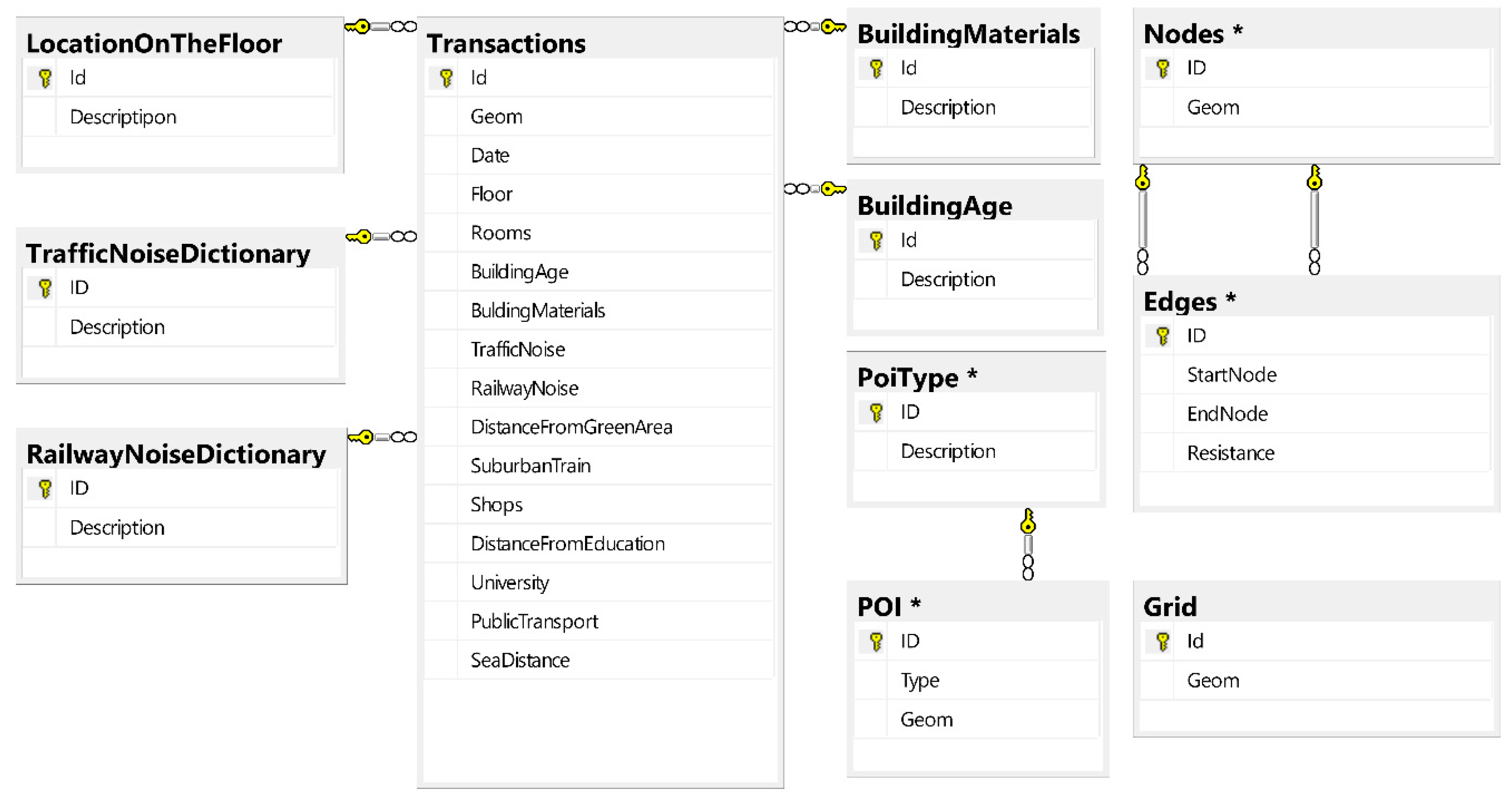
The initial data model (used to build the final version of the production database) was based on data obtained from the public authorities and OSM data imported to the attributes tables. Repeated magnitude of individual attributes has been grouped in order to speed up the classification operations described in further parts of the article. In some cases, these magnitudes have been generalized. The final compilation of the data led to the construction of the normalized form of the relational database shown in Figure 2. It should be noted that four of the tables (transactions, nodes, poi, grid) have a location attributes—fields Geom indicating the location of the transaction referred to the PL–2000 coordinate system (specifically EPSG: 2177).
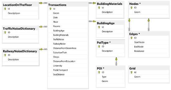
Figure 2.
Database diagram for storing initial observations. Source: Own elaboration.
Most of the imported data did not have a geodetic reference assigned strictly (under EPSG: 2177). It had to be determined solely on the basis of the postal address. Polish postal codes refer to large and irregular areas of the country (not like in the UK) hence the use of geocoding is necessary in such cases. For this purpose, the Nominatim tool was used (to increase the efficiency of the solution) as a part of the same physical machine performing analyses and storing data [49]. The structure indicated in Figure 2, apart from the input data, also contains evaluation fields of the individual transactions’ location. These fields were fed with data derived from spatial analyses carried out on the basis of the scenarios described below. It was also assumed that the final product of analyses is a comprehensive description of the area covered by the analysis—not only described by the observed transactions. The assumed generality of the assessment of the chosen space required uniform coverage of its scope by indicating the value of all the attributes considered. Lack of direct observation in the whole area forced the implementation of an indirect solution. It was based on a proper approximation of the values of these attributes in the nodes of the spatial grid with a square mesh of a = 200 m side (Figure 3).
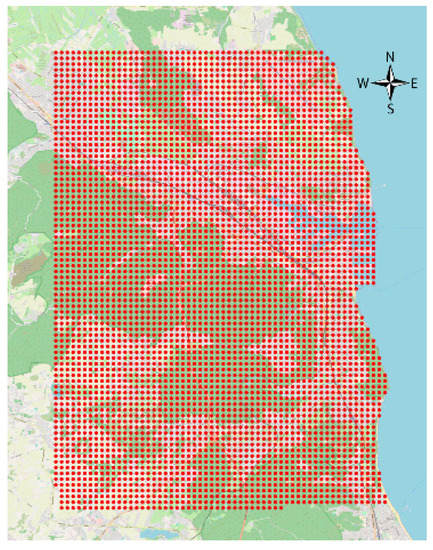
Figure 3.
The range of the study area covered with a rectangular grid with a mesh size of 200m. Source: Own elaboration on Open Street Map (OSM) background and vector data.
This mesh consisted of 4328 nodes (and was stored in table Grid—Figure 2). These nodes did not have strictly assigned attribute magnitude and their determination was based on one of several methods depending on the nature and spatial impact of the attribute. Classical geoinformatics methods for determining a 2D subspace based on topological spatial relations between the integral elements of the environment can use:
- -
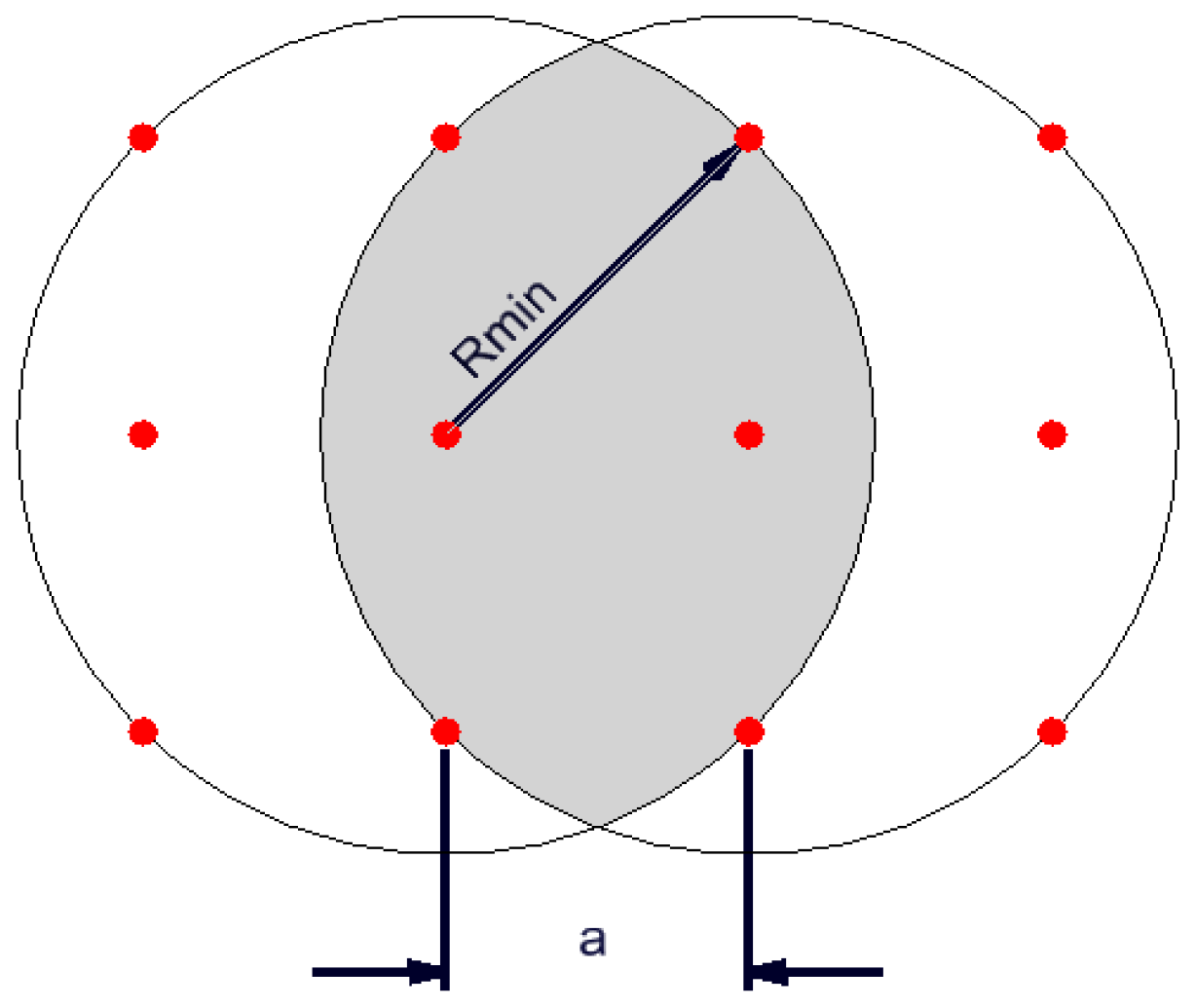
- assessment of the occurrence of a given phenomenon in a spatial buffer zone in the form of a circle with a suitably chosen radius. The assumption of the interpenetration of the impact of individual environmental features on neighbouring grid nodes resulted in the adoption of Rmin = a√2 (Figure 4).
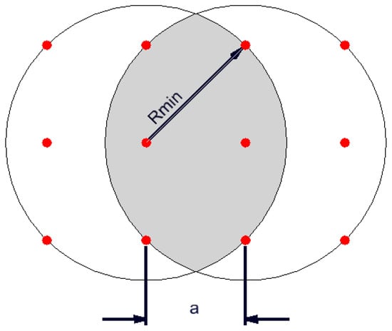 Figure 4. The overlap influence of buffer on the grid nodes. Source: Own elaboration.
 - -
- Euclidean distance—most often recognized as a parameter of the deterministic model. This approach is correct when assessing the proximity of unfavourable factors: noise, pollution sources and so forth. or visual: direct visibility of the sea, where the propagation or nuisance of their impact is a linear dependence on the distance or its derivative,
- -
- other than the numerical and linear nature of the influence of external factors (e.g., location-dependent) on the magnitude of the attribute being examined. From the point of view of functioning in a city, it may often be more important to reach the object of interest than its immediate neighbourhood. The proximity of attractive green areas based on their direct visibility but requiring a by-pass to reach it, loses its significance. In this case, the assessment of the attractiveness of space, comfort of life based on access to “services” of the modern city is based on calculations related to the travel time to such places.
Depending on the access to specific sources and types of data, these calculations may refer to the distance counted along pedestrian, vehicular or public transport routes or compilation of the above. Such information is now available thanks to providers such as Amazon, Google, Microsoft and so forth. They provide the opportunity to enrich information on the attractiveness of real estate by providing real time to reach their destination from the location based on knowledge about the current traffic volume. However, this solution should be used very sensibly due to the changing, not only in the weekly range but also the daily values of available approximations, which raises the problem of assessing the objectivity of calculations. It was decided to make such calculations and include them in the assessment of the attractiveness of urban space. Due to the predicted number of queries to find optimal paths, references to external websites have been abandoned and data from OSM stored locally was used (Tables: Nodes, Edges—Figure 2). The vector resource for OSM roads has been assessed as sufficiently accurate for the required analyses. The resource was pre-narrowed to the analysis space, pedestrian routes were also rejected (the OSM resource is incomplete in this respect). Therefore, the considerations concerned circular availability. The OSM for each road segment polyline contains, among others, information on its type, directionality (one, two-way) and in most cases speed limits (for road sections without this information it was assumed that the speed limit was 50 km/h).
The aforementioned 2D grid coverage with a known spatial reference and the value of the evaluated attributes required for example 8209024 analysis (for calculations of remoteness form the sea). There are ready-made solutions for calculating optimal time-based access paths based on OSRM (Open Source Routing Machine) data. Their use is commonly based on sending http queries to the running pathfinding server. Interoperability based on the use of the TCP/IP connection control of the analysing application, significantly reduces the efficiency of the solution, especially when assuming millions of such analyses for a single, distance-tested attribute. OSRM uses the optimal path search algorithm Dikstrya [50] (de facto Multi-Level Dijkstra) with computational complexity with big O notation of: O(V2) where V is the number of vertices or O(E + V log V)—if a Fibonacci heap was used [51] where E is number of edges.
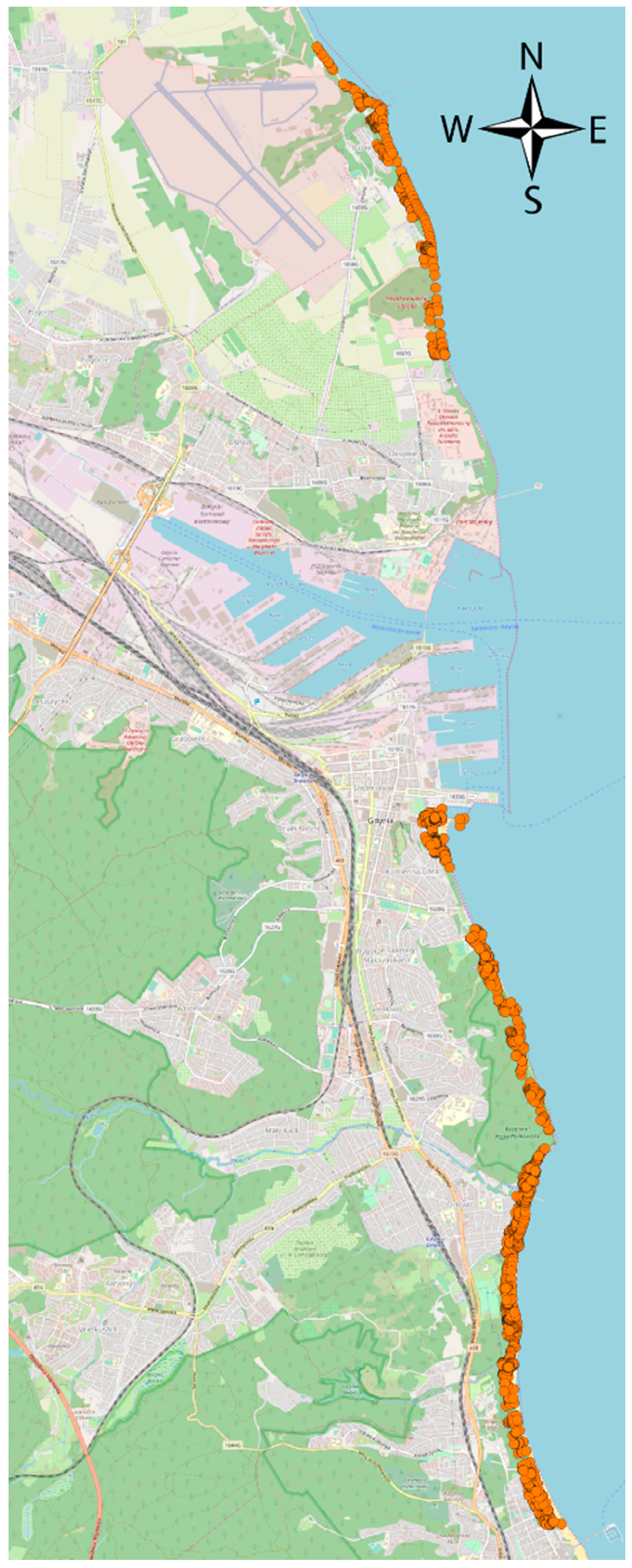
Own prepared application was implemented with the use of the heuristic algorithm A*. Its’ overall computational complexity is O(V + E), because all edges and vertices of the graph need to be stored. The queue implementation of a min–priority kind (Fibonacci heap) only in the worst–case scenario will be O(E + V log V), which is the same as the Dikstrya algorithm. One of the parameters estimated on the basis of the time distance was the time distance of each node of the grid (Figure 3) from the line of direct access to the sea. Starting points were grid nodes and the target 1888 points in the beach zone (designated as points of road breaks within a distance of up to 200 m from the shore line defined at OSM) (Figure 5).
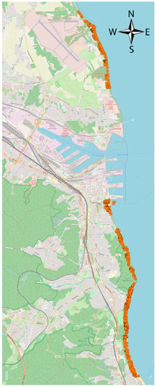
Figure 5.
Visualization of the location of points considered as the target of circular travel to the areas of beaches in Gdynia (orange dots). Source: Own elaboration on OSM background and vector data.
The description of the road network (Tables: Nodes, Edges—Figure 2) was created as a directed graph on the basis of data from the OSM vector resource clipped to the analysed area. Graph consisted of nodes: 390,456 and edges: 23,479. Calculation of 8,209,024 combinations of start pairs, target on a machine with Intel® Core™ processor (Santa Clara, CA, USA) and &–6820HK 2.70 GHz and 32GB RAM was realized within 1 h 28 min. The use of GPU would probably allow for more efficiency—close to real time—but it was not the subject of the theoretical considerations.
Using a discrete regular point description, the analysed area of the city of Gdynia was tested. Areas with the same availability time to the sea (isochrones) were obtained. For that purpose interpolation and quantization methods were used. The chamfered shape (Figure 6) of the contour lines and their course have their spatial, communication, urban and other reasons.
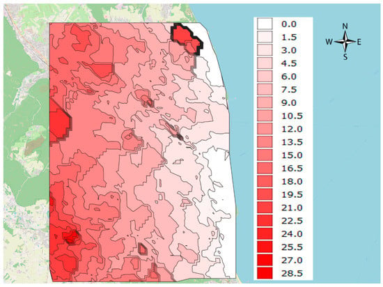
Figure 6.
Isochrones calculated for the time distance from the sea. Source: Own elaboration on OSM background and vector data.
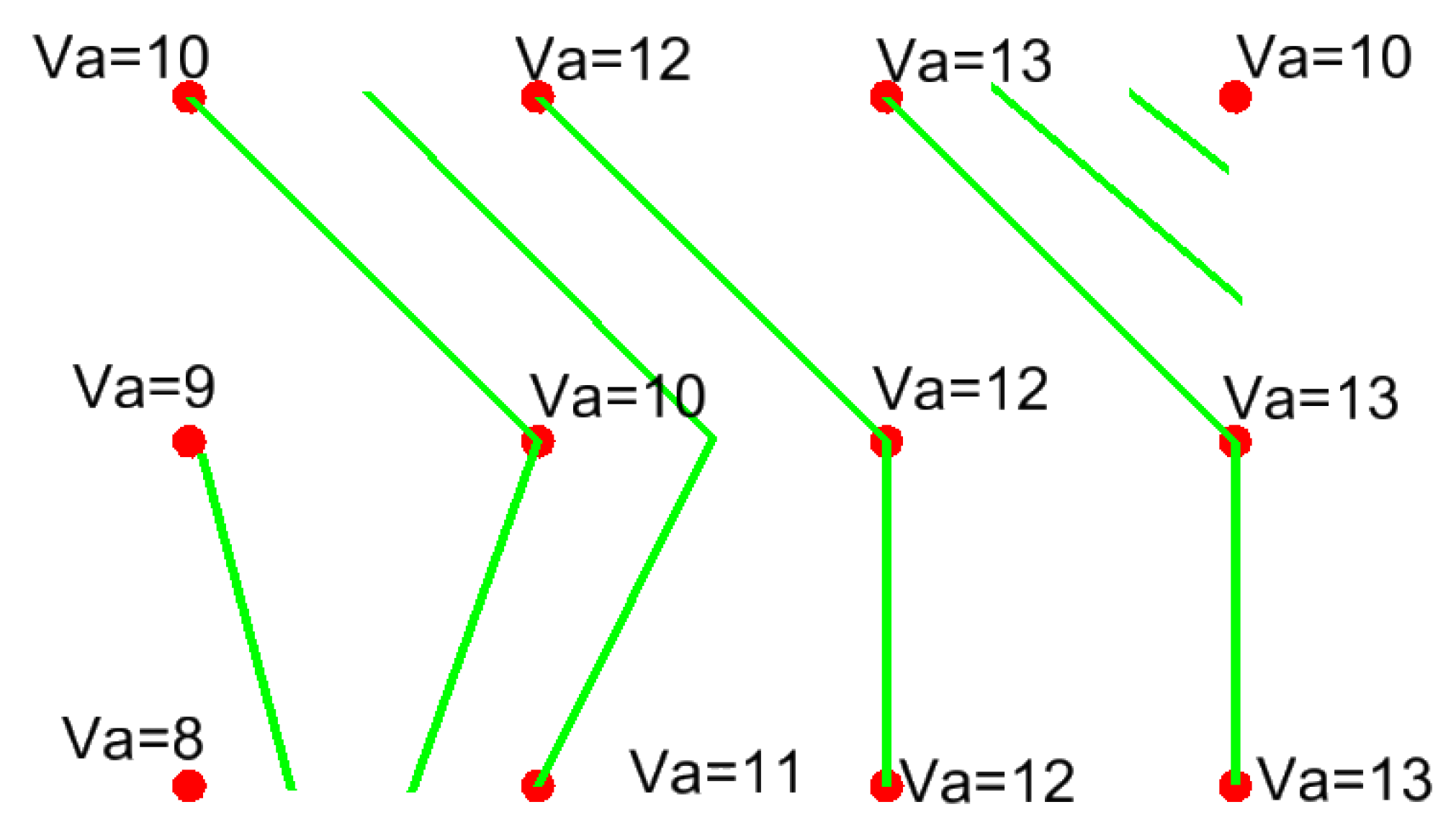
The classical geoinformatics approach to the construction of contours based on a set of points required the implementation of Delaunay triangulation. Due to the systematic and dense grid of points, Delaunay triangulation did not require such a type of processing, even with the use of sophisticated algorithms [52]. The search for contour lines in the form of polylines was assumed. The vertices of these polylines indicated the locations of the same values of the attribute polyline evaluated. The position of vertices with the same values of the analysed attribute was determined on the basis of linear interpolation on sections between adjacent grid nodes (Figure 7).
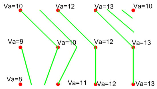
Figure 7.
Determining the trajectory of quasi contours (isochrones). Source: Own elaboration.
These isochrones do not have a perfect smooth character, however, a small distance (200 m) between the nodes of the grid allows to take the size of the arc of the contour line as acceptable for real estate market analyses and at the same time significantly simplifies the construction process of quasi-contours and further numerical analyses.
The point attributes for example schools or public transport stops where elaborated in the similar reference buffer zones but value of centroid where elaborated on the basis of occurred number of particular points of interest’s attraction of property location.
The real estate parameters have been determined with values read from individual layers based on their georeferences. The georeferences were assigned with the use of geocoding due to the fact of having addresses only and not geodetic coordinates.
4.4. Elaboration of the Homogeneous Group of the Property/Transactions
The next stage of the proposed methodology is elaboration of the homogeneous group of the property transactions. The practical problem of data exploration in spatial development results mainly from the non-homogeneity of real estate (no two properties are identical), the presence of various attributes describing real estate (both qualitative and quantitative), a highly diversified access to information on various segments of the real estate market and, frequently, the lack of awareness concerning the dependencies that exist between real estate attributes and market actors. Combined with information overload, imprecision, measurement errors and the unavailability of certain types of information, heteroscedasticity of property geolocation the above factors directly impact the effectiveness of the chosen investigation method and the quality of decisions. This gives rise to a broad scope of utility of this type analyses, related to manners and procedures of designating similarities of real estate markets and properties as such [53].
The specific features of real estate attributes show a high level of variability in the method of each attribute encoding, where key attributes are expressed on a ratio scale, such as the price or area. The coding method should not be modified due to the risk of data loss. In view of the above, the authors have proposed the applications of the fuzzy theory and rough set methods (RST) [54,55,56] to elaborate group of similar (indiscernible) properties. Due to the application of value tolerance relation [57] to the conventional rough set theory based on a crisp indiscernibility relation the more flexible way to deal with the indiscernibility relation was obtained and better match to the real estate market analysis.
Regarding the aim of this study the conditional part of decision table constitute both physical and geolocation attributes, whether the decision attribute is the distance from the spatial decision factor represented by coastal area. In order to group properties that constitute indiscernible (homogeneous) combination the “valued tolerance relation” (VTR) [57] was applied to conditional attributes and the following matrix was created:
where Rj(x,y)—relation between objects (real estates) with a result of membership function [0,1]; x,y—identifier of transaction, cj—function of the j attribute selection from given property, cj(x), cj(y)—homogenous features (attributes of the analysed real estates); j—number of attribute; k—threshold for the homogenous features set, allows objects to be considered indiscernible despite not having identical values; that is standard deviation for data on ratio scale and one interval for data on ordinal scale.
The results produced by the valued tolerance relation matrix of conditional attributes were summed up and the sum matrix was determined based on the below formula:
where pi—real estate/object that is candidate to given homogeneous group (indiscernible).
Assuming that Wx is the collection of all similar (indiscernible) transactions to x, its contents can be described as fulfilment of the following condition:
and
That means that the set of Wx (set of similar transactions to x) consists only that pi from P set, which satisfy the condition defined as a function of the tolerance T.
On this stage, modification of original assumptions of the rough set theory was performed, due to significant variety of the object of analyses. In effect, classes of indiscernibility were determined, taking into account 85% of similarity due to the fact of specificity of the property data that were descripted above. In this stage the formula on the toleration function is as follow:
The degrees of indiscernibility were determined at a given level of similarity for sets in decision subgroups based on the following equation:
where —d attribute in the set of B attributes that are considered indiscernible, i—number of indiscernible set of properties, SI—information system, U—universe of set, it is a non-empty, limited set called universe; elements of the U set are called objects.
After classification of the classes of indiscernibility related to properties the next step assumed elaboration of the group of class the properties indiscernible regarding decision rule (if…then) in the frame of designation the lower approximation that enable establishing the most representative (numerous) set of decision rules.
The mentioned assumptions enable to establish geo-homogenous groups of properties on the basis of the zones related to remoteness from the sea. From this analysis 55 groups of homogeneous property classes based on distance to the coastal area were obtained. After this step the next part of analyses constituted the elaboration of the similar classes of property in terms of physical attributes (312 classes) and attractiveness of geolocation (245 classes).
4.5. Identification Influence of Geolocation on Property Assessment
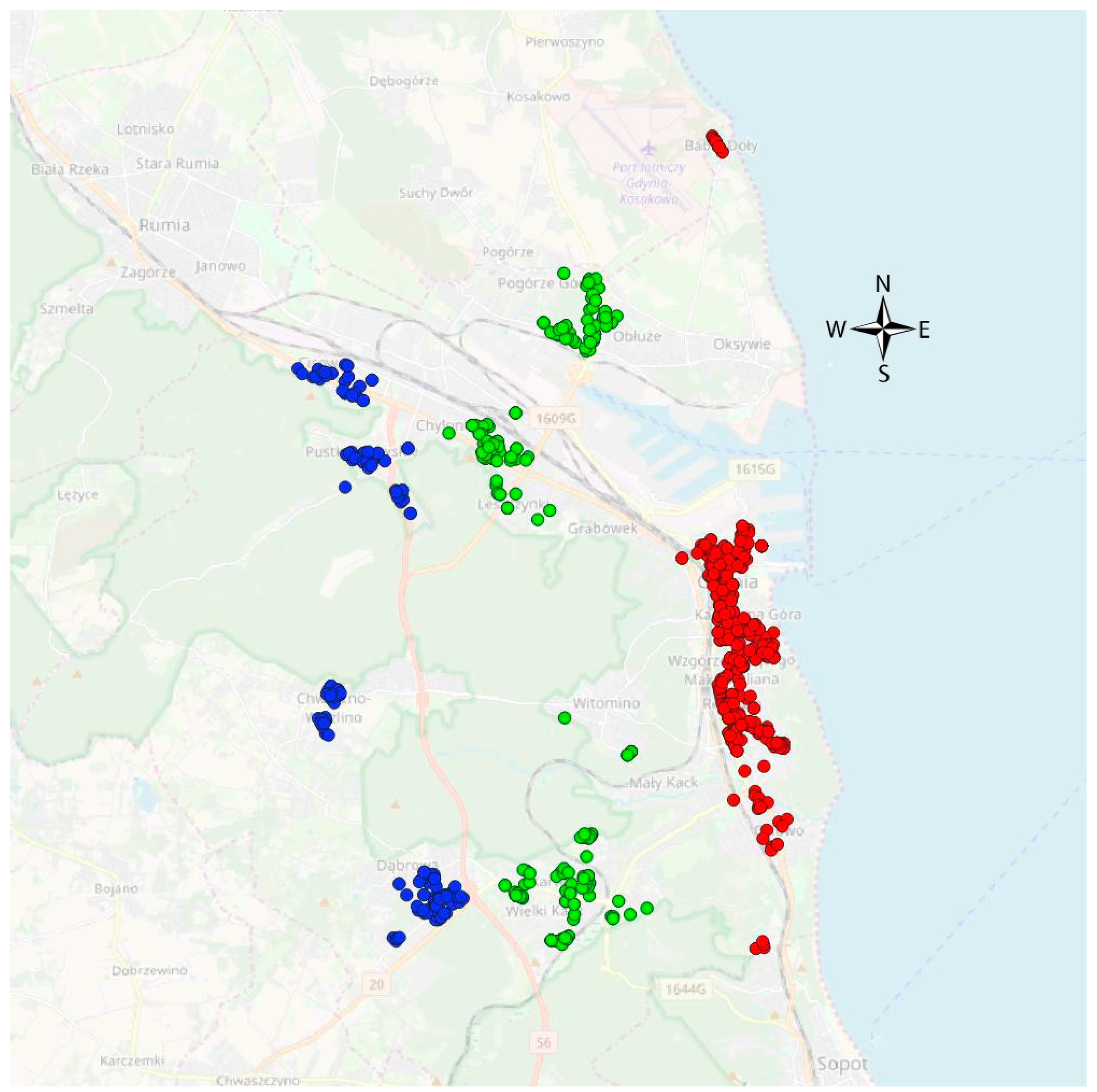
This stage of the procedure involved the determination of the influence of the spatial decision factor on property assessment that was the main purpose of the proposed system. In order to achieve the aim the following stages were conducted. At the very beginning, the analysed area was divided into geo-homogenous groups according to spatial decision attribute that in this case was the remoteness (distance measured in a way described in the previous part of the paper) between the property and the sea. From the number of 55 geo-homogenous property groups (according to the remoteness to the sea) 3 most numerous groups were selected as an example (Figure 8). The presented location of the properties in the three groups (red ones with the smallest remoteness to the sea, blue ones with biggest remoteness to the sea and green ones with medium remoteness) confirms proper division according to the taken criteria.

Figure 8.
The geolocation of the homogeneous property groups according to the spatial decision attribute (red—small remoteness to the sea (zone 1), green—medium remoteness to the sea (zone 2), blue—big remoteness to the sea (zone 3)). Source: own elaboration on OSM background and vector data.
Having designated three geo-homogenous groups according to the spatial decision factor, more detailed (taking into account other attributes) selection was performed (in each of the given three groups). Each group was formed by properties that were similar (according to determined comparability ratio) in terms of both physical and geolocation (other than remoteness to the sea) attributes. That selection enabled obtaining groups that were similar (at a given comparability ratio-85%) in terms of usable area of real estate, building age, building material and others (see Table 1). In order to verify the influence of the remoteness of the sea of particular groups, authors of the paper decided to pick three homogenous groups of properties according to one of the attributes—the building age. The groups were formed by properties located in:
- -
- old buildings (1950–1980),
- -
- building of medium age (1970–1997),
- -
- new buildings (2005–2015).
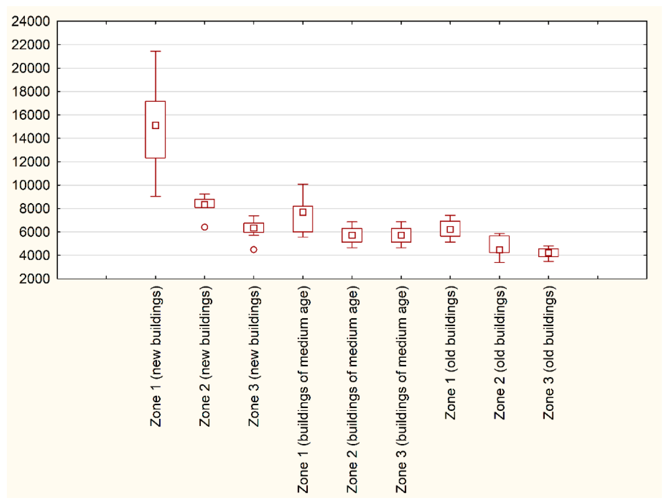
At this stage, what needs to be underlined is that groups determined according to the age of buildings were not equivalent with the division presented in Table 1. The location of representative three groups according to building age was prepared and presented in Figure 9. In order to illustrate the influence of the remoteness of the sea on properties values the box plot within each of the given three groups according to the age of properties was prepared and presented in Figure 10.
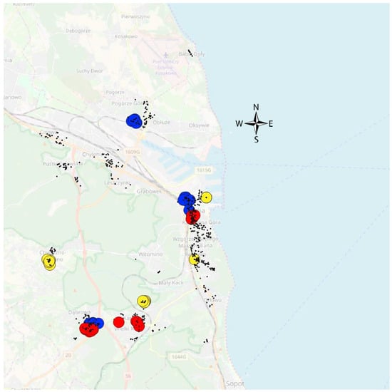
Figure 9.
Representative properties in homogeneous groups according to physical and geolocation attributes in three building age groups (red—old buildings, yellow—buildings of medium age, blue—new buildings). Source: own elaboration on OSM background and vector data.
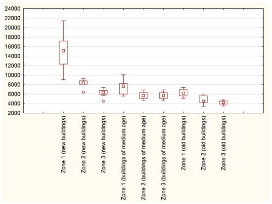
Figure 10.
The influence of remoteness of the sea on property values within the three groups of properties divided according to the age of the building. Source: own elaboration.
What has been noticed (Figure 10) was that in the case of every group, either these were new buildings, buildings of medium age or old buildings, the noticed relationship was that the bigger the distance from the sea, the lower property price. The biggest interquartile range has been noticed in the group of new building located in zone 1 (the smallest remoteness to the sea). That confirms the attractiveness of the geolocation of properties in Gdynia the coastal areas.
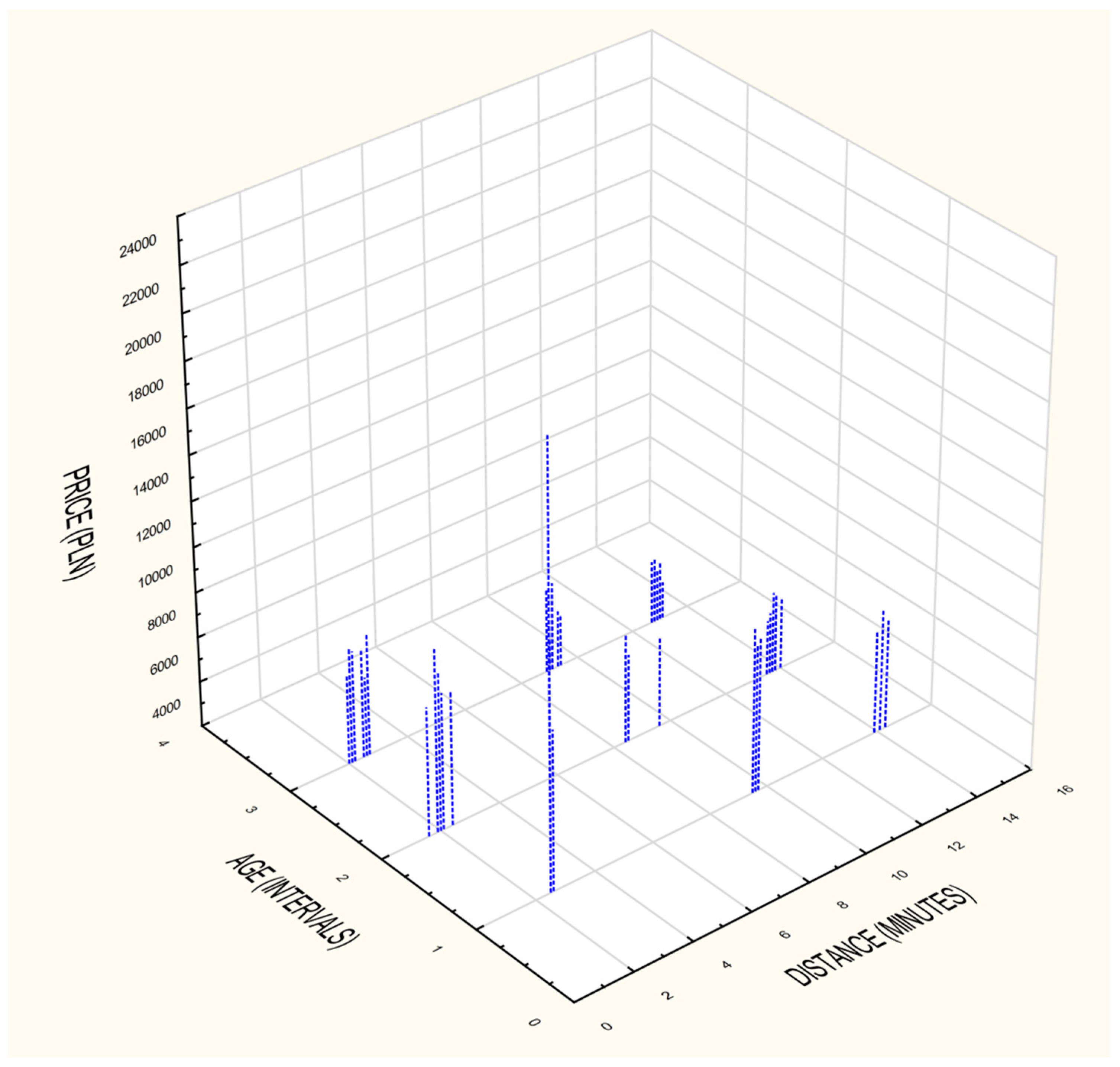
Taking an in depth look at the variables presented in numeral (price, distance) and interval (age) scales (Figure 11), it has been noticed that the prices of properties ranged from approximately 9000 PLN per square meter up to 21,000 PLN per square meter. The significant diversity of the prices, in one case was caused by the luxurious character of given apartments located in one building (the Sea Towers). In the case of other groups, the interquartile range was much smaller, nevertheless showing the same relation of influence of the remoteness to the sea on property prices. In order to confirm the obtained results authors additionally prepared spectral graph to present the relationship (Figure 11).
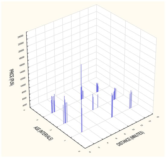
Figure 11.
The influence of remoteness of the sea on property values building. Source: own elaboration.
The last step of the analysis involved the determination of the remoteness to the sea on property prices without the concept of AMV. In order to do so, the methods used in individual valuations (proposed by International Valuation Standards) were applied. Even though the theory of property valuation presents many formulas involving the determination of the influence of particular property attributes on their prices, in order to calculate the influence of the remoteness to the sea, the authors of the paper used the interval method based on ceteris paribus assumption. The formula is as follows:
where:
- CW—unit price brought to the valuation date of the highest condition of the feature,
- CM—unit price with the lowest condition.
The denominator in the formula presented above is the price difference, which is calculated on the basis of the formula:
where:
- CMAX—the highest recorded unit price in the set
- CMIN—the lowest unit price recorded in the set.
The influence of the remoteness to the sea on the prices of selected groups of properties (Table 2) is presented in the Table 3. The influence was presented in PLN, which provides the particular difference in property prices depending on the remoteness.

Table 2.
The selected group of properties used for determination of remoteness to the sea influence on property prices.

Table 3.
The influence on property prices of remoteness to the sea on selected group of properties.
The interval method used in individual valuations confirmed big differences in the achieved results. The conclusions drawn from those results confirm a lack of objectivity in the methods. The comparison of results that equal 0.17 and 0.74, based on the subjective selection of compared transactions, leaves big room for doubts in terms of objectivity deduction. The prices of the properties varied significantly in every group, so the influence of the sea remoteness in each group was also diversified. The results confirm the fundamental character of the real estate market and transactions that are connected with uncertainty. Even though the proposed decision support system enabled the objective classification of similar properties, the prices among comparable groups differed.
5. Discussion and Conclusions
The developed structures and methodologies of automated real estate analysis methods should take into particular account their connotations with space and the influence of geolocation factors on their classification, value, or the way they are used. The analysis of the real estate market and decision making in relation to real estate is subject to high uncertainty due to, among other things, the specific character of the information that describes it and the difficulty in defining the strength of the influence of individual factors.
The proposed solutions within the elaboration support decision system on the real estate market with the use of geo-technologies enabled the flexibility and scalability by frequent modifications of spatial (geolocation) connotation. The flexibility in this case should be interpreted as the possibility of adjusting to the model of the analysed data that is crucial for the property market.
Use of the geoscience method is not new in property analyses; however, specific approaches and solutions are different and can shed new light on the existing solutions. The problem is that the analysed data in the real estate market has a discrete (not continuous) character. The spatial analyses that enable improvement in the accuracy, and a decrease in the uncertainty of the obtained results required information which described the area of interest in the continuous way. In this study, the authors provided original solutions and proposed results taking into account the mentioned conditions.
The results confirming the influence of the spatial decision factor—in this case remoteness of the sea—have shown that, on average, the value of properties located in new buildings in the first zone (the smallest remoteness to the sea) in comparison with properties located in new buildings but in the second zone, which were 35% lower. The smallest difference noticed within the analysed properties was between properties located in old buildings in zones 2 and 3 and equalled 22%.
Further study will focus on identifying the attractiveness of property geolocation with respect to behavioural aspects. Interesting results may be achieved regarding the confusion of perception (often stereotypes) of geolocation with real conditions and the attractiveness of a given space. This is important from the point of view of participants in real estate turnover that determine the final price of the property. The problem in question concerns the fact that these are the participants who create the real estate market to a large extent, while their awareness and objective knowledge increases.
Author Contributions
The authors contributed equally to the research.
Funding
This research received no external funding.
Conflicts of Interest
The authors declare no conflict of interest.
References
- Von Bertalanffy, L. General System Theory; George Braziller, Inc.: New York, NY, USA, 1968. [Google Scholar]
- Demetriou, D. Automating the land valuation process carried out in land consolidation schemes. Land Use Policy 2018, 75, 21–32. [Google Scholar] [CrossRef]
- Źróbek, S.; Grzesik, C. Modern Challenges Facing the Valuation Profession and Allied University Education in Poland. Real Estate Manag. Valuat. 2013, 21, 14–18. [Google Scholar] [CrossRef]
- Kriegel, H.P.; Schneider, R.; Brinkhoff, T. Potentials for improving query processing in spatial databse systems. Proc. 9iemes Journees Bases Donnees Avoncee 1993, 11, 11–31. [Google Scholar]
- Prigogine, I.; Stengers, I. Order out of Chaos: Man’s New Dialogue with Nature; Bantam Books: New York, NY, USA, 1984; ISBN 9780553340822. [Google Scholar]
- Popper, K. The Logic of Scientific Discovery; Routledge: London, UK, 2002. [Google Scholar]
- Longley, P.; Higgs, G.; Martin, D. The predictive use of GIS to model property valuations. Int. J. Geogr. Inf. Syst. 1994, 8, 217–235. [Google Scholar] [CrossRef]
- Wyatt, P. The development of a property information system for valuation using geographical information system (GIS). J. Prop. Res. 1996, 13, 317–336. [Google Scholar] [CrossRef]
- Hamilton, S.; Morgan, A. Integrating lidar, GIS and hedonic price modeling to measure amenity values in urban beach residential property markets. Comput. Environ. Urban Syst. 2010, 34, 133–141. [Google Scholar] [CrossRef]
- Gedal, M.; Ellen, I.G. Valuing urban land: Comparing the use of teardown and vacant land sales. Reg. Sci. Urban Econ. 2018, 70, 190–203. [Google Scholar] [CrossRef]
- Cupal, M. Flood Risk as a Price–setting Factor in the Market Value of Real Property. Procedia Econ. Financ. 2015, 23, 658–664. [Google Scholar] [CrossRef]
- Renigier–Biłozor, M.; Biłozor, A.; Wiśniewski, R. Real estate markets rating engineering as the condition of urban areas assessment. Land Use Policy 2017, 61, 511–525. [Google Scholar] [CrossRef]
- Robinson, G.; Dawnie, M. Integrating valuation models with valuation services to meet the need of borrowers lenders and valuers. Find. Built Rural. Environ. 2009, 3, 3–10. [Google Scholar]
- RICS. Comparable Evidence in Property Valuation; RICS: London, UK, 2012; ISBN 978-1-84219-684. [Google Scholar]
- Renigier–Biłozor, M.; Wiśniewski, R.; Biłozor, A.; Kaklauskas, A. Rating methodology for real estate markets–Poland case study. Int. J. Strateg. Prop. Manag. 2014, 18, 198–212. [Google Scholar] [CrossRef]
- Mark, J.; Goldberg, M. Multiple regression analysis and mass assessment: A review of the issue. Apprais. J. 1988, 56, 89–109. [Google Scholar]
- Fletcher, M.; Gallimore, P.; Mangan, J. Heteroscedasticity in hedonic house price models. J. Prop. Res. 2000, 17, 93–108. [Google Scholar] [CrossRef]
- Dubin, R.A.; Goodman, A.C. Valuation of neighborhood characteristics through hedonic prices. Popul. Environ. 1982, 5, 166–181. [Google Scholar] [CrossRef]
- Des Rosiers, F.; Theriault, M. House Prices and Spatial Dependence: Towards an Integrated Procedure to Model Neighbourhood Dynamics; Working Papiers; Laval–Faculte des Sciences de Administration: Rue de la Terrasse, QC, Canada, 1999. [Google Scholar]
- Helbich, M.; Brunauer, W.; Vaz, E.; Nijkamp, P. Spatial heterogeneity in hedonic house price models: The case of Austria. Urban Stud. 2014, 51, 390–411. [Google Scholar] [CrossRef]
- Radhakrishna, R.C. Statistics and Truth: Putting Chance to Work; World Scientific: Singapore, 1997. [Google Scholar]
- Ferretti, V.; Montibeller, G. Key challenges and meta–choices in designing and applying multi–criteria spatial decision support systems. Decis. Support Syst. 2016, 84, 41–52. [Google Scholar] [CrossRef]
- Malczewski, J. GIS–based land–use suitability analysis: A critical overview. Prog. Plan. 2004, 62, 3–65. [Google Scholar] [CrossRef]
- Borst, R.; McCluskey, W. The Modified Comparable Sales Method as the Basis for a Property Tax Valuations System and Its Relationship and Comparison to Spatially Autoregressive Valuation Models; Kauko, T., d’Amato, M., Eds.; Mass Appraisal Methods: An International Perspective for Property Valuers; Wiley Blackwell: Chicester, UK, 2008; pp. 49–69. [Google Scholar] [CrossRef]
- Wilhelmsson, M. Spatial models in real estate economics. Hous. Theory Soc. 2002, 19, 92–101. [Google Scholar] [CrossRef]
- Borst, R.A.; McCluskey, W.J. Comparative evaluation of the comparable sales method with geostatistical valuation models. Pac. Rim Prop. Res. J. 2007, 13, 106–129. [Google Scholar] [CrossRef]
- Quintos, C. Spatial weight matrices and their use as baseline values and location–adjustment factors in property assessment models. Cityscape 2013, 15, 295–306. [Google Scholar]
- d’Amato, M.; Kauko, T. Advances in Automated Valuation Modeling: AVM after the Non–Agency Mortgage Crisis; Springer: Heidelberg, Germany, 2017. [Google Scholar]
- Lentz, G.H.; Wang, K. Residential appraisal and the lending process: A survey of issues. J. Real Estate Res. 1998, 15, 11–39. [Google Scholar]
- Renigier–Biłozor, M. Analysis of real estate markets with the use of the rough set theory. J. Pol. Real Estate Sci. Soc. 2011, 19, 107–118. [Google Scholar]
- Borst, R.A. Artificial Neural Networks: The Next Modelling/Calibration Technology for the Assessment Community. Prop. Tax J. 1992, 10, 69–94. [Google Scholar]
- McCluskey, W.; Deddis, W.; Mannis, A.; McBurney, D.; Borst, R. Interactive application of computer assisted mass appraisal and geographic information systems. J. Prop. Valuat. Invest. 1997, 15, 448–465. [Google Scholar] [CrossRef]
- Worzala, E.; Lenk, M.; Silva, A. An Exploration of Neural Networks and its Application to Real Estate Valuation. J. Real Estate Res. 1995, 10, 185–201. [Google Scholar]
- O’Connor, P. Automated valuation models by model–building practitioners: Testing hybrid model structure and GIS location adjustments. J. Prop. Tax Assess. Adm. 2008, 5, 5–24. [Google Scholar]
- Jozaghi, A.; Alizadeh, B.; Hatami, M.; Flood, I.; Khorrami, M.; Khodaei, N.; Tousi, E. A Comparative Study of the AHP and TOPSIS Techniques for Dam Site Selection Using GIS: A Case Study of Sistan and Baluchestan Province, Iran. Geosciences 2018, 8, 494. [Google Scholar] [CrossRef]
- d’Amato, M. A comparison between MRA and rough set theory for mass appraisal. A case in bari. Int. J. Strateg. Prop. Manag. 2004, 8, 205–217. [Google Scholar] [CrossRef]
- Aurelio, M.; Gonzalez, S. Automated Valuation Methods in Real Estate Market–a Two–Level Fuzzy System; d’Amato, M., Kauko, T., Eds.; Advances in Automated Valuation Modeling; AVM after the Non–Agency Morgage Crisis; Springer: Berlin, Germany, 2017; ISBN 978-3-319-49746-4. [Google Scholar]
- Kauko, T.; d’Amato, M. Neighbourhood Effect, International Encyclopedia of Housing and Home; Elsevier Publisher: Cambridge, UK, 2011. [Google Scholar]
- PricewaterhouseCoopers. Available online: https://www.pwc.pl/en/wielkie-miasta-polski/raport_tricity_eng.pdf (accessed on 14 March 2019).
- Kaklauskas, A.; Kelpsiene, L.; Zavadskas, E.K.; Bardauskiene, D.; Kaklauskas, G.; Urbonas, M.; Sorakas, V. Crisis management in construction and real estate: Conceptual modeling at the micro–, meso– and macro–levels. Land Use Policy 2011, 28, 280–293. [Google Scholar] [CrossRef]
- Ball, M.; Wood, A. Housing investment: Long run international trends and volatility. Hous. Stud. 1999, 14, 185–209. [Google Scholar] [CrossRef]
- Case, K.E.; Shiller, R.J. Forecasting Prices and Excess Returns in the Housing Market. Real Estate Econ. 1990, 18, 253–273. [Google Scholar] [CrossRef]
- Cellmer, R.; Bełej, M.; Zrobek, S.; Subic-Kovac, M. Urban Land Value Maps—A Methodological Approach. Geod. Vestn. 2014, 58, 535–551. [Google Scholar] [CrossRef]
- McCue, D.; Belsky, E.S. Why do House Prices Fall? Perspective on the Historical Drivers of Large Nominal House Price Declines; Joint Center for Housing Studies of Harvard University: Cambridge, MA, USA, 2007. [Google Scholar]
- Kaklauskas, A.; Zavadskas, E.K.; Trinkunas, V. A multiple criteria decision support on–line system for construction. Eng. Appl. Artif. Intell. 2007, 20, 163–175. [Google Scholar] [CrossRef]
- Zhang, Z.; Lu, X.; Zhou, M.; Song, Y.; Luo, X.; Kuang, B. Complex spatial morphology of urban housing price based on digital elevation model: A case study of wuhan city, china. Sustainability 2019, 11, 348. [Google Scholar] [CrossRef]
- Noichan, R.; Dewancker, B. Analysis of accessibility in an urban mass transit node: A case study in a bangkok transit station. Sustainability 2018, 10, 819. [Google Scholar] [CrossRef]
- Goodchild, M.F. A Geographer Looks at Spatial Information Theory; Montello, D.R., Ed.; Spatial Information Theory; COSIT 2001; Lecture Notes in Computer Science; Springer: Berlin, Germany, 2001; Volume 2205. [Google Scholar]
- Clemens, K. Geocoding with OpenStreetMap Data. In Proceedings of the Seventh International Conference on Advanced Geographic Information Systems, Applications, and Services, Lisbon, Portugal, 22–27 February 2015. [Google Scholar]
- Dijkstra, E.W. A Note on Two Problems in Connexion with Graphs. Numer. Math. 1959, 1, 269–271. [Google Scholar] [CrossRef]
- Reddy, H. Path Finding–Dijkstra’s and A* Algorithm’s”, December 13, 2013. Available online: http://cs.indstate.edu/hgopireddy/algor.pdf (accessed on 14 March 2019).
- Yang, S.W.; Choi, Y.; Jung, C.K. A divide–and–conquer Delaunay triangulation algorithm with a vertex array and flip operations in two–dimensional space. Int. J. Precis. Eng. Manuf. 2011, 12, 435–442. [Google Scholar] [CrossRef]
- Renigier-Biłozor, M.; Biłozor, A. The Significance of Real Estate Attributes in the Process of Determining Land Function with the Use of the Rough Set Theory; Scientific Monograph: Value in the Process of Real Estate Management and Land Administration; Studia i Materiały Towarzystwa Naukowego Nieruchomości: Olsztyn, Poland, 2009; pp. 103–117. ISBN 978-83-61564-00-3. [Google Scholar]
- Pawlak, Z. Rough sets. Int. J. Inf. Comput. Sci. 1982, 11, 341–356. [Google Scholar] [CrossRef]
- Komorowski, J.; Pawlak, Z.; Polkowski, L.; Skowron, A. Rough Sets: A Tutorial; Pal, S.K., Skowron, A., Eds.; Rough Fuzzy Hybrydatin; A New Trend in Decision Making; Springer: Berlin, Germany, 1999; pp. 3–98. [Google Scholar]
- Zadeh, L.A. Fuzzy sets. Inf. Control 1965, 8, 338–352. [Google Scholar] [CrossRef]
- Stefanowski, J.; Tsoukias, A. Valued Tolerance and Decision Rules. In International Conference on Rough Sets and Current Trends in Computing; Ziarko, W., Yao, Y., Eds.; Springer: Berlin, Germany, 2000. [Google Scholar]
© 2019 by the authors. Licensee MDPI, Basel, Switzerland. This article is an open access article distributed under the terms and conditions of the Creative Commons Attribution (CC BY) license (http://creativecommons.org/licenses/by/4.0/).

